The high-order block RIP for non-convex block-sparse compressed sensingThanks: Corresponding author, E-mail: wjjmath@gmail.com, wjj@swu.edu.cn(J.J. Wang), E-mail: hjw1303987297@126.com (J. Huang)

Block-sparse signal recovery (BSR) appears in some fields of sparse modelling and machine learning, including color imaging [13], equalization of sparse communication channels [2], multi-response linear regression [3] and imagine annotation [4] and so forth. Essentially, the important problem in BSR is how to reconstruct a block-sparse or approximately block-sparse signal from a linear system. Commonly, one thinks over the below model:

$\displaystyle y=\Phi x+e,$

where $y\in\mathbb{R}^{n}$ is the observation measurement, $\Phi\in\mathbb{R}^{n\times N}$ is a known measurement matrix (or sensing matrix) with $n<N$, and $e\in\mathbb{R}^{n}$ is a vector of measurement errors. Generally, the conventional compressed sensing (CS) simply thinks out the sparsity of the signal to be recovered, however it doesn’t consider any additional structure, i.e., non-zero elements appear in blocks (or clusters) rather than being arbitrarily spread all over the vector. We call these signals as the block-sparse signals. In order to define block sparsity, we need to give several additional notations. Suppose that the signal $x$ over the block index set $\mathcal{I}=\{d_{1},d_{2},\cdots,d_{M}\}$, then we can describe the signal $x$ as

$\displaystyle x=[\underbrace{x_{1},\cdots,x_{d_{1}}}_{x[1]},\underbrace{x_{d_{1}+1},\cdots,x_{d_{1}+d_{2}}}_{x[2]},\cdots,\underbrace{x_{N-d_{M}+1},\cdots,x_{N}}_{x[M]}]^{\top},$

(1.1)

where $x[i]$ represents the $i$th block of $x$ and $N=\sum^{M}_{i=1}d_{i}$. We call a vector $x$ as block $s$-sparse over $\mathcal{I}=\{d_{1},d_{2},\cdots,d_{M}\}$ if $x[i]$ is non-zero for no more than $s$ indices $i$ [5]. In fact, if the block-sparse structure of signal is neglected, the conventional CS doesn’t efficiently treat such structured signal. To reconstruct block-sparse signal, researchers [5] [6] proposed the following mixed $l_{2}/l_{1}$-minimization:

$\displaystyle\hat{x}=\arg\min_{\tilde{x}\in\mathbb{R}^{N}}\|\tilde{x}\|_{2,\mathcal{I}}~\mbox{s.t.}~y-\Phi\tilde{x}\in\mathcal{B},$

(1.2)

where $\|x\|_{2,\mathcal{I}}=\sum^{M}_{i=1}\|x[i]\|_{2}$ is the mixed $l_{2}/l_{1}$ norm of a vector $x$. The set $\mathcal{B}$ stands for some noise structure,

$\displaystyle\mathcal{B}^{l_{2}}(\rho):=\{e:~\|e\|_{2}\leq\rho\}$

(1.3)

and

$\displaystyle\mathcal{B}^{DS}(\rho):=\{e:~\|\Phi^{\top}e\|_{\infty}\leq\rho\},$

(1.4)

where $\Phi^{\top}$ represents the conjugate transpose of the matrix $\Phi$. (1.2) is a convex optimization issue and could be converted into a second-order cone program, so can be solved efficiently.

To study the theoretical performance of mixed $l_{2}/l_{1}$-minimization, Eldar and Mishali [5] proposed the definition of block restricted isometry property (block RIP).

For the reminder of this paper, for simplicity, $\delta_{s}$ represents the block RIP constant $\delta_{s|\mathcal{I}}$. Eldar and Mishali [5] showed that the mixed $l_{2}/l_{1}$-minimization method can exactly reconstruct any block $s$-sparse signal when the measurement matrix $\Phi$ fulfills the block RIP with $\delta_{2s}<0.414$. Later, Lin and Li [7] improved the sufficient condition on $\delta_{2s}$ to $0.4931$, and builded condition $\delta_{s}<0.307$ for accurate recovery. In 2019, the conclusions of literature [8] and [9] together present a complete characterization to the block RIP condition on $\delta_{ts}$ that the mixed $l_{2}/l_{1}$ minimization method guarantees the block-sparse signal recovery in the field of block-sparse compressed sensing.

Recently, a lot of researchers [10] [11] [12] have revealed that $l_{p}~(0<p<1)$ minimization not only constantly needs less constrained the RIP requirements, but also could ensure exact recovery for smaller $p$ compared with the $l_{1}$ minimization. In the present paper, we are interested in investigating the stable reconstruction of block-sparse signals by the mixed $l_{2}/l_{p}~(0<p<1)$ minimization as follows:

$\displaystyle\hat{x}=\arg\min_{\tilde{x}\in\mathbb{R}^{N}}\|\tilde{x}\|^{p}_{2,p}~\mbox{s.t.}~y-\Phi\tilde{x}\in\mathcal{B},$

(1.6)

where $\|x\|^{p}_{2,p}=\sum^{M}_{i=1}\|x[i]\|^{p}_{2}$. Simulation experiments [13] [14] indicated that fewer linear measurements are needed for accurate reconstruction when $0<p<1$ than when $p=1$. More related work can be found in literature [15] [16] [17] [18] [19] [20] [21].

In this paper, we further investigate the high-order block RIP conditions for the exact and stable reconstruction for (approximate) block-sparse signals by mixed $l_{2}/l_{p}$ minimization. The crux is extend sparse representation of an $l_{p}$-polytope (Lemma 2.2 [22]) to the block scenario. With this technique, we obtain a sufficient condition on RIC $\delta_{ts}$ that guarantees the exact and stable reconstruction of approximate block-sparse signals via mixed $l_{2}/l_{p}$ minimization, and establish error bounds between the solution to (1.6) and the signal $x$ to be recovered. Obviously, when $x$ is accurately block-sparse and $\mathcal{B}=\{0\}$ (i.e., $y=\Phi x$), we will derive the accurate reconstruction condition. Particularly, we will determine how many random Gaussian measurements suffice for the condition to hold with high probability.

The remainder of the paper is constructed as follows. In Section 2, we will provide some notations and a few lemmas. In Section 3, we will present the main results, and the associating proofs are given in Section 5. In Section 4, a series of numerical experiments are presented to support our theoretical results. Lastly, the conclusion is drawn in Section 6.

Throughout this article, we use the below notations unless special mentioning. For a subset $T$ in $\mathbb{R}^{M}$, $T^{c}$ denotes the complement of $T$ in $\mathbb{R}^{M}$. For any vector $x\in\mathbb{R}^{N}$, $x_{T}$ represents a vector which is equal to $x$ on block indices $T$ and displaces other blocks with zero. Denote $T_{0}$ by block indices of the $s$ largest block in $l_{2}$ norm of the vector $x$, i.e., $\|x[i]\|_{2}\geq\|x[j]\|_{2}$ for any $i\in T_{0}$ and $j\in T^{c}_{0}$. We represent $x_{\max(s)}$ as $x$ with all but the largest $s$ blocks in $l_{2}$ norm set to zero. Henceforth, we invariably choose that $h=\hat{x}-x_{\max(s)}$, where $\hat{x}$ is the minimizer of (1.6).

In order to prove our main results, it is necessary to present the below lemma which is a crucial technical tool. Factually, we extend sparse expression of an $l_{p}$-polytope proposed by [22] to the block context.

We will utilize the below lemma in the process of proving the main conclusions, which is a useful important inequality.

In view of the definition of $h$, $\hat{x}$ and $x_{\max(s)}$, we get the below lemma.

Based on the knowledge prepared above, we present the main results in this part-a high-order block RIP condition for the robust reconstruction of arbitrary signals with block structure via mixed $l_{2}/l_{p}$ minimization. In the case that the signal to be recovered is block-sparse, the condition can respectively guarantee the accurate construction and stable recovery in the noise-free case and in the noise situation. When the original signal $x$ is not block-sparse and the linear measurement is corrupted by noise, the below result presents a sufficient condition for recovery of structured signals.

In the following, we will decide how many random Gaussian measurements are demanded for (3.1) to be fulfilled with overwhelming probability. In this sequel, let $(\Omega,\tau)$ be a probability measure space and $z$ be a random variable which follows one of the following probability distributions:

$\displaystyle z\sim\mathcal{N}(0,1/n),~z\sim\begin{cases}1/\sqrt{n},\quad\ \ &\mbox{w.p.}~1/2,\\ -1/\sqrt{n},\quad\ \ &\mbox{w.p.}~1/2,\end{cases}\mbox{or}~z\sim\begin{cases}\sqrt{3/n},\quad\ \ &\mbox{w.p.}~1/6,\\ 0,\quad\ \ &\mbox{w.p.}~2/3,\\ -\sqrt{3/n},\quad\ \ &\mbox{w.p.}~1/6.\end{cases}$

(3.6)

Given $n$ and $N$, the random matrices $\Phi$ can be produced by making choice of the elements $\Phi_{i,j}$ as independent copies of $z$. This generates the random matrices $\Phi$.

In this section, we carry out a few numerical simulations to hold out the application of our theoretical results. We could transform the constrained optimization problem (1.6) into an alternative unconstrained form below:

$\displaystyle\min_{\tilde{x}\in\mathbb{R}^{N}}\lambda\|\tilde{x}\|^{p}_{2,p}+\frac{1}{2}\|y-\Phi\tilde{x}\|^{2}_{2}.$

(4.1)

Solving the problem (4.1), we adopt the standard Alternating Direction Method of Multipliers (ADMM)[27][28][26]. Utilizing a auxiliary variable $v\in\mathbb{R}^{N}$, we can rewrite the formulation (4.1) as

$\displaystyle\min_{\tilde{x},~v\in\mathbb{R}^{N}}\lambda\|v\|^{p}_{2,p}+\frac{1}{2}\|y-\Phi\tilde{x}\|^{2}_{2}~\mbox{s.t.}~\tilde{x}-v=0.$

(4.2)

The augmented Lagrangian function of the above problem is

$\displaystyle\mathcal{L}_{\gamma}(\tilde{x},v,z)=\lambda\|v\|^{p}_{2,p}+\frac{1}{2}\|y-\Phi\tilde{x}\|^{2}_{2}+\left<z,\tilde{x}-v\right>+\frac{\gamma}{2}\|\tilde{x}-v\|^{2}_{2},$

(4.3)

where $z\in\mathbb{R}^{n}$ is a Lagrangian multiplier, and $\gamma>0$ is a penalty parameter. Then, ADMM composes of the below three steps:

		$\displaystyle\tilde{x}^{k+1}=\arg\min\frac{1}{2}\|y-\Phi\tilde{x}\|^{2}_{2}+\frac{\gamma}{2}\|z^{k}+\tilde{x}-v^{k}\|^{2}_{2}$		(4.4)
		$\displaystyle v^{k+1}=\arg\min\lambda\|v\|^{p}_{2,p}+\frac{\gamma}{2}\|z^{k}+\tilde{x}^{k+1}-v\|^{2}_{2}$		(4.5)
		$\displaystyle z^{k+1}=z^{k}+\tilde{x}^{k+1}-v^{k+1}.$		(4.6)

The solution of problem (4.4) is explicitly provided by

$\displaystyle\tilde{x}^{k+1}=(\Phi^{\top}\Phi+\gamma I_{n})^{-1}(\Phi^{\top}y-\gamma(z^{k}-v^{k})).$

(4.7)

To use the existing conclusions on the proximity operator of $l_{p}$-norm ($0<p<1$), by employing the inequality: $\|x\|_{2}<\|x\|_{p}$ for $x\in\mathbb{R}^{n}$ and $0<p<1$, the optimization problem (4.5) can be converted into

$\displaystyle v^{k+1}=\arg\min\sum^{M}_{i=1}\lambda\|v[i]\|^{p}_{p}+\frac{\gamma}{2}\|z^{k}[i]+\tilde{x}^{k+1}[i]-v[i]\|^{2}_{2}.$

(4.8)

In our experiments, without loss of generality, we think over the block-sparse signal $x$ with even block size, i.e., $d_{i}=d$, $i=1,\cdots,M$, and take the signal length $N=1024$. For each experiment, first of all, we randomly produce block-sparse signal $x$ with the amplitude of each nonzero entry generated according to the Gaussian distribution. We use an $n\times N$ orthogonal Gaussian random matrix as the measurement matrix $\Phi$. We set the number of random measurement $m=128$ unless otherwise specified. With $x$ and $\Phi$, we generate the linear measurement $y$ by $y=\Phi x+e$, where $e$ is the Gaussian noise vector. Each given experimental result is an average over 100 independent trails.

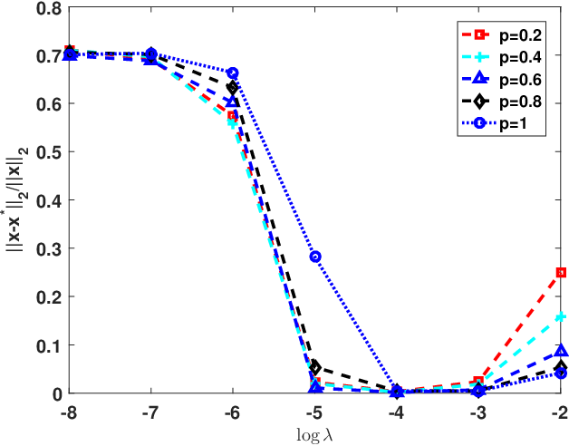
In Fig. 1a, we produce the signals by making choice of $64$ blocks uniformly at random with $n=64,~N=128$, i.e., the block size $d=2$. The relative error of recovery $\|x-x^{*}\|_{2}/\|x\|_{2}$ is plotted versus the regularization parameter $\lambda$ for the different values of $p$, i.e., $p=0.2,~0.4,~0.6,~0.8,~1$. The $\lambda$ ranges from $10^{-8}$ to $10^{-2}$. From the figure, the parameter $\lambda=10^{-4}$ is a proper choice. Fig. 1b presents experimental results regarding the performance of the non-block algorithm and the block algorithm with $p=0.4$. Two curves of relative error are provided via mixed $l_{2}/l_{p}$ minimization and orthogonal greedy algorithm (OGA) [29]. Fig. 1b reveals the signal construction is quite significant in signal recovery.

Signal-to-noise ratio (SNR, SNR$=20\log_{10}(\|x\|_{2}/\|x-x^{*}\|_{2})$) versus the values of $p$ and the nonzero entries $k$, the results are respectively given in Fig. 2a and b. In Fig. 2a, the values of $p$ vary from $0.01$ to $1$, and in Fig. 2b, the number of nonzero entries $k$ ranges from $8$ to $48$. Figs. 2a and b evidences that mixed $l_{2}/l_{p}$ minimization performs better than that of standard $l_{p}$ minimization. Figs. 2a and b provide the relationship between the relative error and the number of measurements $n$ in different block sizes $d=1,~2,~4,~8$ and the values of $p=0.2,~0.4,~0.6,~0.8,~1$.

Eventually, we compare the performance of Group-Lp for $p=0.4$ with other typical algorithms consisting of Block-OMP algorithm[30], Block-SL0 algorithm [31] for $l_{2}/l_{0}$ solver and Block-ADM algorithm [32]. We exploit SNR to weigh the algorithm efficiency. In Fig. 4a, we select signals whose block size $d=2,~4,~8,~16,~32$ with the number of nonzero entries $k=32$ as the test signals, and in Fig. 4b, the block size $d=2$. One can see that, overall, the performance of Group-Lp ($p=0.4$) is much better than that of other three algorithms.

Denote $\alpha^{p}=\|h_{\max(s)}\|^{p}_{2,p}/s$. Then, by utilizing Lemma 2.3, we have

		$\displaystyle\|h_{-\max(s)}\|_{2,\infty}\leq\alpha\leq\frac{\alpha}{(t-1)^{1/p}},~\mbox{and}$
		$\displaystyle\|h_{-\max(s)}\|^{p}_{2,p}\leq s(t-1)\left(\frac{\alpha}{(t-1)^{1/p}}\right)^{p}.$		(5.1)

Through applying Lemma 2.1 and combining with (5), we have $h_{-\max(s)}=\sum^{N}_{i=1}\lambda_{i}u_{i}$, where $u_{i}$ is block $(t-1)s$-sparse, $\sum^{N}_{i=1}\lambda_{i}=1$ with $\lambda_{i}\in[0,1]$, and

$\displaystyle\sum_{i}\lambda_{i}\|u_{i}\|^{2}_{2,2}\leq\frac{\alpha^{p}}{t-1}\|h_{-\max(s)}\|^{2-p}_{2,2-p}.$

(5.2)

Hence,

	$\displaystyle\sum_{i}\lambda_{i}\|u_{i}\|^{2}_{2,2}$	$\displaystyle\overset{\text{(a)}}{\leq}\frac{\alpha^{p}}{t-1}\left(\|h_{-\max(s)}\|^{2}_{2,2}\right)^{\frac{2(1-p)}{2-p}}\left(\|h_{-\max(s)}\|^{p}_{2,p}\right)^{\frac{p}{2-p}}$
		$\displaystyle\leq\frac{\alpha^{p}}{t-1}\left(\|h_{-\max(s)}\|^{2}_{2,2}\right)^{\frac{2(1-p)}{2-p}}(s\alpha^{p})^{\frac{p}{2-p}}$
		$\displaystyle\overset{\text{(b)}}{\leq}\frac{1}{t-1}\left(\|h_{-\max(s)}\|^{2}_{2,2}\right)^{\frac{2(1-p)}{2-p}}\left(\|h_{\max(s)}\|^{2}_{2,2}\right)^{\frac{p}{2-p}}$
		$\displaystyle\overset{\text{(c)}}{\leq}\frac{1}{t-1}\left(\|h_{-\max(s)}\|^{2}_{2}\right)^{\frac{2(1-p)}{2-p}}\left(\|h_{\max(s)}\|^{2}_{2}\right)^{\frac{p}{2-p}},$		(5.3)

where (a) follows from H$\ddot{o}$lder’s inequality, (b) is due to the fact that $\|x\|_{p}\leq\|x\|_{q}\leq n^{1/q-1/p}\|x\|_{p}$, $x\in\mathbb{R}^{n}$ and given $0<q<p\leq\infty$, and (c) is from the fact that $\|x\|^{2}_{2,2}=\sum^{M}_{i=1}\|x[i]\|^{2}_{2}=\sum^{N}_{i=1}x_{i}^{2}=\|x\|^{2}_{2}$, $x\in\mathbb{R}^{N}$.

From Cauchy-Schwartz inequality and the definition of block RIP, we get

$\displaystyle\left<\Phi h_{\max(s)},\Phi h\right>\leq\|\Phi h_{\max(s)}\|_{2}\|\Phi h\|_{2}\leq\sqrt{1+\delta_{ts}}\|h_{\max(s)}\|_{2}\|\Phi h\|_{2}.$

(5.4)

Since

	$\displaystyle\|\Phi h\|_{2}$	$\displaystyle\leq\|\Phi(\hat{x}^{l_{2}}-x_{\max(s)})\|_{2}\leq\|\Phi\hat{x}^{l_{2}}-y\|_{2}+\|\Phi x_{\max(s)}-y\|_{2}$
		$\displaystyle\leq\varepsilon+\rho+\sigma(\Phi)\|x_{-\max(s)}\|_{2},$		(5.5)

therefore

$\displaystyle\left<\Phi h_{\max(s)},\Phi h\right>\leq\sqrt{1+\delta_{ts}}(\varepsilon+\rho+\sigma(\Phi)\|x_{-\max(s)}\|_{2})\|h_{\max(s)}\|_{2}.$

(5.6)

Take $\beta_{i}=h_{\max(s)}+(t-1)\mu u_{i}$. Then,

$\displaystyle\sum^{N}_{j=1}\lambda_{j}\beta_{j}-\frac{p}{2}\beta_{i}-(t-1)\mu h=\left[1-(t-1)\mu-\frac{p}{2}\right]h_{\max(s)}-\frac{p}{2}(t-1)\mu u_{i}.$

(5.7)

Furthermore, both $\sum^{N}_{j=1}\lambda_{j}\beta_{j}-\frac{p}{2}\beta_{i}-(t-1)\mu h$ and $\beta_{i}-\beta_{j}=(t-1)\mu(u_{i}-u_{j})$ are block $ts$-sparse, because $h_{\max(s)}$ is block $s$-sparse, and $u_{i}$ is block $(t-1)s$-sparse.

References

• [1] A. Majumdar , R. Ward ,Compressed sensing of color images, Signal Process. 90 (2010) 3122-3127.
• [2] F. Parvaresh , H. Vikalo , S. Misra , B. Hassibi , Recovering sparse signals using sparse measurement matrices in compressed DNA microarrays, IEEE J. Sel. Top- ics Signal Process. 2 (3) (2008) 275-285 .
• [3] S. Cotter , B. Rao , Sparse channel estimation via matching pursuit with applica- tion to equalization, IEEE Trans. Commun. 50 (3) (2002) 374-377 .
• [4] J. Huang , X. Huang , D. Metaxas , Learning with Dynamic Group Sparsity, in: IEEE 12th International Conference on Computer Vision, 2009, pp. 64-71 .
• [5] Y. Eldar , M. Mishali , Robust recovery of signals from a structured union of sub- spaces, IEEE Trans. Inf. Theory 55 (11) (2009) 5302-5316 .
• [6] Y. Eldar , P. Kuppinger , H. Bolcskei , Block-sparse signals: uncertainty relations and efficient recovery, IEEE Trans. Signal Process. 58 (6) (2010) 3042-3054 .
• [7] J. Lin , S. Li , Block sparse recovery via mixed l2/l1l_{2}/l_{1} minimization, Acta Mathe- matica Sinica 29 (7) (2013) 1401-1412 .
• [8] Li Y, Chen W. The high order block RIP condition for signal recovery[J]. Journal of Computational Mathematics, 2019, 37(1): 61-75.
• [9] Huang J, Wang J, Wang W, et al. Sharp sufficient condition of block signal recovery via l2/l1l_{2}/l_{1}-minimisation[J]. IET Signal Processing, 2019, 13(5): 495-505.
• [10] R. Chartrand , V. Staneva , Restricted isometry properties and nonconvex compressive sensing, Inverse Probl. 24 (2008) 1-14 .
• [11] Y. Shen , S. Li , Restricted p -isometry property and its application for nonconvex compressive sensing, Adv. Comput. Math. 37 (2012) 441-452 .
• [12] M. Lai , Y. Xu , W. Yin , Improved iteratively reweighted least squares for unconstrained smoothed l q minimization, SIAM J. Numer. Anal. 51 (2) (2013) 927-957 .
• [13] A. Majumdar , R. Ward ,Compressed sensing of color images, Signal Process. 90 (2010) 3122-3127 .
• [14] Y. Wang , J. Wang , Z. Xu , On recovery of block-sparse signals via mixed l2/lq​(0<q≤1)l_{2}/l_{q}~(0<q\leq 1) norm minimization, EURASIP J. Adv. Signal Process. 76 (2013) 1-17 .
• [15] Y. Wang , J. Wang , Z. Xu , Restricted pp-isometry properties of nonconvex block-sparse compressed sensing, Signal Process. 104 (2014) 188-196 .
• [16] Wen J, Zhou Z, Liu Z, et al. Sharp sufficient conditions for stable recovery of block sparse signals by block orthogonal matching pursuit[J]. Applied and Computational Harmonic Analysis, 2019, 47(3): 948-974.
• [17] Gao Y, Peng J, Yue S. Stability and robustness of the l2/lql_{2}/l_{q}-minimization for block sparse recovery[J]. Signal Processing, 2017, 137: 287-297.
• [18] Wang J, Huang J, Zhang F, et al. Group sparse recovery in impulsive noise via alternating direction method of multipliers[J]. Applied and Computational Harmonic Analysis, 2019.
• [19] Ge H, Chen W. Recovery of signals by a weighted l2/l1l_{2}/l_{1} minimization under arbitrary prior support information[J]. Signal Processing, 2018, 148: 288-302.
• [20] Haifeng Li and Jinming Wen. A New Analysis for Support Recovery With Block Orthogonal Matching Pursuit, IEEE Signal Processing Letters, 26(2019), 247-251.
• [21] Wang W, Wang J, Zhang Z. Block-sparse signal recovery via l2/l1−2l_{2}/l_{1-2} minimisation method[J]. IET Signal Processing, 2017, 12(4): 422-430.
• [22] Zhang R, Li S. Optimal RIP bounds for sparse signals recovery via lpl_{p} minimization[J]. Applied and Computational Harmonic Analysis, 47(2019)566-584.
• [23] T.T. Cai, A. Zhang, Sharp RIP bound for sparse signal and low-rank matrix recovery, Appl. Comput. Harmon. Anal., 35 (2013), 74-93.
• [24] Chen B, Wan A. General RIP bounds of δt​k\delta_{tk} for sparse signals recovery by lpl_{p} minimization[J]. Neurocomputing, 2019, 363: 306-312.
• [25] Baraniuk R, Davenport M, DeVore R, et al. A simple proof of the restricted isometry property for random matrices[J]. Constructive Approximation, 2008, 28(3): 253-263.
• [26] Lu C, Feng J, Lin Z, et al. Exact low tubal rank tensor recovery from Gaussian measurements[C]. Proceedings of the 27th International Joint Conference on Artificial Intelligence. AAAI Press, 2018: 2504-2510.
• [27] Wen F, Liu P, Liu Y, et al. Robust Sparse Recovery in Impulsive Noise via ℓp\ell_{p}-ℓ1\ell_{1} Optimization[J]. IEEE Transactions on Signal Processing, 2017, 65(1): 105-118.
• [28] Wen F, Pei L, Yang Y, et al. Efficient and robust recovery of sparse signal and image using generalized nonconvex regularization[J]. IEEE Transactions on Computational Imaging, 2017, 3(4): 566-579.
• [29] Petukhov A. Fast implementation of orthogonal greedy algorithm for tight wavelet frames[J]. Signal processing, 2006, 86(3): 471-479.
• [30] Eldar Y C, Kuppinger P, Bolcskei H. Block-sparse signals: Uncertainty relations and efficient recovery[J]. IEEE Transactions on Signal Processing, 2010, 58(6): 3042-3054.
• [31] Ghalehjegh S H, Babaie-Zadeh M, Jutten C. Fast block-sparse decomposition based on SL0[C]. International Conference on Latent Variable Analysis and Signal Separation. Springer, Berlin, Heidelberg, 2010: 426-433.
• [32] Deng W, Yin W, Zhang Y. Group sparse optimization by alternating direction method[C]. Wavelets and Sparsity XV. International Society for Optics and Photonics, 2013, 8858: 88580R.