AoI-optimal Joint Sampling and Updating for Wireless Powered Communication Systems

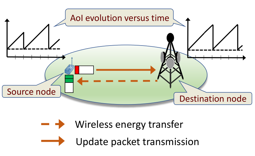
We consider a single source-destination pair model in which the source contains: i) a sensor that keeps sampling the real-time status of a physical process and ii) a transmitter that sends status update packets about the observed process to the destination, as shown in Fig. 1. Since the single source-destination pair model may actually be sufficient to study a diverse set of applications [2] (e.g., safety of an intelligent transportation system, predicting and controlling forest fires, and efficient energy utilization in future smart homes), our analysis in this paper will be of interest in many applications. The scenario of having multiple source nodes is left as a promising direction of future work.

We assume that the source node may perform sophisticated sampling tasks, e.g., initial feature extraction and pre-classification using machine learning tools [12]. Hence, unlike most of the existing literature, the time and energy costs of generating an update packet at the source node cannot be neglected. While the destination node is assumed to be always connected to the power grid, the source node is powered through WET by the destination node. Particularly, the destination node transmits RF signals in the downlink to charge the source node. The energy harvested by the source node is then stored in its battery, which has a finite capacity of $B_{\rm max}$ joules. The source and destination nodes share the same channel and they have a single antenna each. Hence, the source can either harvest energy or transmit data at a given time instant.

We assume discrete time and the time slots are of equal size. Let $B(n)$, $A(n)$ and $\tau(n)$ denote the amount of available energy in the battery at the source node, the AoI at the destination node, and the time passed since the generation instant of the current update packet available at the source node (i.e., the AoI of the status updates at the source node), respectively, at the beginning of time slot $n$. Denote by $h(n)$ and $g(n)$ the uplink and downlink channel power gains between the source and destination nodes over slot $n$, respectively. We assume that the channels are influenced by quasi-static flat fading. This, in turn, means that the channels are fixed over a time slot, and independently vary from one slot to another.

The state of the system at slot $n$ can be expressed as $s(n)\triangleq\left(B\left(n\right),A\left(n\right),\tau\left(n\right),h\left(n\right),g\left(n\right)\right)\in{\mathbb{S}}$; where ${\mathbb{S}}$ is the state space which contains all the combinations of the system state variables. We also assume that the state variables can take discrete values²² 2 Note that constructing a finite state space of an MDP by discretizing the state variables and/or defining upper bounds on their maximum values is very common in the literature to obtain the optimal policy numerically as well as characterize its structure properties analytically using standard optimization techniques such as the Value Iteration Algorithm (VIA) or Policy Iteration Algorithm (PIA). See [12, 22, 23, 28] for representative examples. and obtain a lower bound to the performance of the continuous system (as it will be clear in the sequel). In particular, we have $B(n)\in\{0,1,\cdots,b_{\rm max}\}$ where $b_{\rm max}$ denotes the battery capacity, such that each energy quantum in the battery is equivalent to $e_{\rm q}=\frac{B_{\rm max}}{b_{\rm max}}$ joules. Note that both the energy consumed from the battery for an update packet transmission and the harvested energy need to be expressed in terms of the energy quanta. In addition, if the channel power gains are originally modeled using continuous random variables, we discretize them into a finite number of intervals whose probabilities are determined from the probability density function (PDF) of the fading gain. In particular, each interval is then represented by a discrete level of channel power gain which has the same probability as that of this interval. Without loss of generality, we also assume that $A(n)$ $(\tau(n))$ is upper bounded by a finite value $A_{\rm max}$ $(\tau_{\rm max})$ which can be chosen to be arbitrarily large [12, 22]. When $A(n)$ reaches $A_{\rm max}$, it means that the available information at the destination node is too stale to be of any use.

Based on $s(n)$, two actions are decided at slot $n$: i) the first action $a_{1}(n)\in{\mathbb{A}}_{1}\triangleq\{S,I\}$ determines whether the source generates a new update packet in slot $n$ or not, and ii) the second action $a_{2}(n)\in{\mathbb{A}}_{2}\triangleq\{T,H\}$ determines whether slot $n$ is allocated for an update packet transmission from the source to the destination or WET by the destination. Specifically, when $a_{1}(n)=S$, a new update packet is generated by the source, which replaces the currently available one, if any, since there is no benefit of sending out-of-date packets to the destination. We also consider that generating an update packet takes one time slot (as a time cost) and requires an amount of energy $E^{\rm S}$ (as energy cost expressed in energy quanta). When $a_{2}(n)=T$, the source sends its currently available packet (that was generated from $\tau(n)$ time slots) to the destination. The required energy for a packet transmission of size $M$ bits in slot $n$, according to Shannon’s formula, is $E^{\rm T}(n)=\frac{\sigma^{2}}{h(n)}\left(2^{M/W}-1\right)$, where $\sigma^{2}$ is the noise power at the destination and $W$ is the channel bandwidth. When $a_{2}(n)=H$, slot $n$ is allocated for WET by the destination to charge the battery at the source. We consider a practical non-linear energy harvesting model [29] such that the energy harvested by the source is given by

where $a$ and $b$ are constants representing the steepness and the inflexion point of the curve that describes the input-output power conversion, $P_{\rm max}$ is the maximum power that can be harvested through a particular circuit configuration, and $P_{\rm rec}(n)=P_{\rm t}g(n)$ such that $P_{\rm t}$ is the average transmit power by the destination. Hence the system action at slot $n$ can be expressed as $a\left(n\right)=\left(a_{1}\left(n\right),a_{2}\left(n\right)\right)\in{\mathbb{A}}={\mathbb{A}}_{1}\times{\mathbb{A}}_{2}$, where ${\mathbb{A}}$ is the action space of the system.

Note that the system state is assumed to be available at the destination node at the beginning of each time slot to take decisions. In particular, we assume that the location of the source node is known a priori, and hence the average channel power gains are pre-estimated and known at the destination node. In particular, at the beginning of an arbitrary time slot, the destination node has perfect knowledge about the channel power gains in that slot, and only a statistical knowledge for future slots [28]. Further, given some initial values for the remaining system state parameters (i.e., $B(0)$, $\tau(0)$ and $A(0)$), the destination node updates their values based on the action taken at each time slot. More specifically, $B(n+1)$ can be expressed as a function of the system action at slot $n$ $(a(n))$ as

where we used the ceiling and floor with $E^{\rm T}(n)$ and $E^{\rm H}(n)$, respectively. Thus, we obtain a lower bound to the performance of the original continuous system. An upper bound can be obtained by reversing the ceiling and floor operators. Let ${\mathbb{A}}\left(s\left(n\right)\right)$ denote the action space associated with state $s(n)$, i.e., ${\mathbb{A}}\left(s\left(n\right)\right)$ contains the possible actions that can be taken at $s(n)$. We assume that $a(n)\in{\mathbb{A}}\left(s\left(n\right)\right)$ only if $B(n)$ is greater than the energy required for taking action $a(n)$, hence we always have $B(n+1)\geq 0$. Furthermore, $A(n+1)$ and $\tau(n+1)$ can be expressed, respectively, as

where $a(n)=(a_{1}(n),T)$ means that $a(n)\in\{(I,T),(S,T)\}$. This also applies to $(S,a_{2}(n))$ w.r.t. $a_{2}(n)$.

A policy is a mapping from the system state space to the system action space. Under a policy $\pi$, the long-term average AoI at the destination with initial state $s(0)$ is given by

We take the expectation w.r.t. the channel conditions and policy in (5). We then aim at finding the policy $\pi^{*}$ that achieves the minimum average AoI, i.e.,

Owing to the independence of channel power gains over time and the nature of the dynamics of remaining state variables, as described by (2)-(4), the problem can be modeled as an MDP. Recall that the system state space is finite (the state variables are discretized) and the system action space is clearly finite as well. In this case, the MDP at hand is a finite-state finite-action MDP, for which there exists an optimal stationary deterministic policy (i.e., we take a deterministic action at each state that is fixed over time) that can be obtained using the VIA or PIA [30]. Therefore, in the sequel, we omit the time index and explore this stationary deterministic policy. In the next section, we characterize the AoI-optimal policy $\pi^{\star}$ and derive its structural properties.

Given a stationary deterministic policy $\pi$, the probability of moving from state $s=(B,A,\tau,h,g)$ to state $s^{\prime}=(B^{\prime},A^{\prime},\tau^{\prime},h^{\prime},g^{\prime})$ can be expressed as

where $\pi(s)$ denotes the action taken at state $s$ according to $\pi$, $\mathbb{P}(h^{\prime})$ and $\mathbb{P}(g^{\prime})$ denote the probability mass functions for the uplink and downlink channel power gains, and $C=\mathbb{P}\left(h^{\prime}\right)\mathbb{P}\left(g^{\prime}\right)$. Step (a) follows since the channel power gains are independent over time from each other and from other random variables. Note that for the case of a Markovian fading channel model, the conditional probabilities $\mathbb{P}(h^{\prime}\left.\right|h)$ and $\mathbb{P}(g^{\prime}\left.\right|g)$ will replace $\mathbb{P}(h^{\prime})$ and $\mathbb{P}(g^{\prime})$, respectively. These conditional probabilities are determined according to the Markovian fading channel model considered in the problem. However, all our analytical results regarding the structure of the AoI-optimal policy (derived in the next subsection) will remain the same. Step (b) follows due to the fact that given $s$ and $\pi(s)$, we can obtain $B^{\prime}$, $A^{\prime}$ and $\tau^{\prime}$ in a deterministic way separately from each other using (2)-(4). The optimal policy $\pi^{\star}$ can be characterized using following Lemma.

The value function $V(s)$ can be obtained iteratively using the VIA [30]. Particularly, according to the VIA, the value function at iteration $k$, $k=1,2,\cdots$, is evaluated as

where $s\in{\mathbb{S}}$. Hence, $\pi^{\star}(s)$ at iteration $k$ is given by

Note that in each iteration of the VIA, the optimal action at each system state needs to be computed using (12) (this is referred to as the policy improvement step). Under any initialization of value function $V(s)^{(0)}$, according to the VIA, the sequence $\left\{V(s)^{(k)}\right\}$ converges to $V(s)$ which satisfies the Bellman’s equation in (8), i.e.,

In the next subsection, we will use the VIA to explore the structural properties of $\pi^{\star}$, which will be exploited to reduce the computational complexity of the VIA (as will be demonstrated in Remark 2). Note that the obtained analytical results can be derived using Relative VIA (RVIA) as well [30].

References

- [1] M. A. Abd-Elmagid, N. Pappas, and H. S. Dhillon, “On the role of age of information in the Internet of things,” IEEE Commun. Magazine, vol. 57, no. 12, pp. 72–77, 2019.
- [2] S. Kaul, R. Yates, and M. Gruteser, “Real-time status: How often should one update?” in Proc., IEEE INFOCOM, 2012.
- [3] R. Talak, S. Karaman, and E. Modiano, “Minimizing age-of-information in multi-hop wireless networks,” in Proc., Allerton Conf. on Commun., Control, and Computing, 2017.
- [4] B. Buyukates, A. Soysal, and S. Ulukus, “Age of information in Two-hop multicast networks,” in Proc., IEEE Asilomar, 2018.
- [5] I. Kadota, E. Uysal-Biyikoglu, R. Singh, and E. Modiano, “Minimizing the age of information in broadcast wireless networks,” in Proc., Allerton Conf. on Commun., Control, and Computing, 2016.
- [6] M. Bastopcu and S. Ulukus, “Who should google scholar update more often?” in Proc., IEEE INFOCOM Workshops, 2020.
- [7] M. K. Abdel-Aziz, C.-F. Liu, S. Samarakoon, M. Bennis, and W. Saad, “Ultra-reliable low-latency vehicular networks: Taming the age of information tail,” in Proc., IEEE Globecom, 2018.
- [8] A. Kosta, N. Pappas, and V. Angelakis, “Age of information: A new concept, metric, and tool,” Foundations and Trends in Networking, 2017.
- [9] Y. Sun, I. Kadota, R. Talak, and E. Modiano, “Age of information: A new metric for information freshness,” Synthesis Lectures on Communication Networks, 2019.
- [10] Y. Gu, H. Chen, Y. Zhou, Y. Li, and B. Vucetic, “Timely status update in internet of things monitoring systems: An age-energy tradeoff,” IEEE Internet of Things Journal, vol. 6, no. 3, pp. 5324–5335, 2019.
- [11] M. A. Abd-Elmagid and H. S. Dhillon, “Average peak age-of-information minimization in UAV-assisted IoT networks,” IEEE Trans. on Veh. Technology, vol. 68, no. 2, pp. 2003–2008, Feb 2019.
- [12] B. Zhou and W. Saad, “Joint status sampling and updating for minimizing age of information in the Internet of Things,” IEEE Trans. on Commun., vol. 67, no. 11, pp. 7468–7482, 2019.
- [13] M. A. Abd-Elmagid, A. Ferdowsi, H. S. Dhillon, and W. Saad, “Deep reinforcement learning for minimizing age-of-information in UAV-assisted networks,” in Proc., IEEE Globecom, 2019.
- [14] P. D. Mankar, Z. Chen, M. A. Abd-Elmagid, N. Pappas, and H. S. Dhillon, “Throughput and age of information in a cellular-based iot network,” 2020, available online: arxiv.org/abs/2005.09547.
- [15] E. Fountoulakis, N. Pappas, M. Codreanu, and A. Ephremides, “Optimal sampling cost in wireless networks with age of information constraints,” in Proc., IEEE INFOCOM Workshops, 2020.
- [16] M. A. Abd-Elmagid, M. A. Kishk, and H. S. Dhillon, “Joint energy and SINR coverage in spatially clustered RF-powered IoT network,” IEEE Trans. on Green Commun. and Networking, vol. 3, no. 1, pp. 132–146, March 2019.
- [17] R. D. Yates, “Lazy is timely: Status updates by an energy harvesting source,” in Proc., IEEE ISIT, 2015.
- [18] B. T. Bacinoglu, E. T. Ceran, and E. Uysal-Biyikoglu, “Age of information under energy replenishment constraints,” in Proc., IEEE ITA, 2015.
- [19] X. Wu, J. Yang, and J. Wu, “Optimal status update for age of information minimization with an energy harvesting source,” IEEE Trans. on Green Commun. and Networking, vol. 2, no. 1, pp. 193–204, 2018.
- [20] S. Feng and J. Yang, “Age of information minimization for an energy harvesting source with updating erasures: With and without feedback,” 2018, available online: arxiv.org/abs/1808.05141.
- [21] A. Arafa and S. Ulukus, “Timely updates in energy harvesting two-hop networks: Offline and online policies,” IEEE Trans. on Wireless Commun., vol. 18, no. 8, pp. 4017–4030, Aug. 2019.
- [22] E. T. Ceran, D. Gündüz, and A. György, “Reinforcement learning to minimize age of information with an energy harvesting sensor with harq and sensing cost,” in Proc., IEEE INFOCOM Workshops, 2019.
- [23] G. Stamatakis, N. Pappas, and A. Traganitis, “Control of status updates for energy harvesting devices that monitor processes with alarms,” in Proc., IEEE GLOBECOM Workshops, 2019.
- [24] O. Ozel, “Timely status updating through intermittent sensing and transmission,” 2020, available online: arxiv.org/abs/2001.01122.
- [25] Y. Lu, K. Xiong, P. Fan, Z. Zhong, and K. B. Letaief, “Optimal online transmission policy in wireless powered networks with urgency-aware age of information,” in Proc., IEEE IWCMC, 2019.
- [26] I. Krikidis, “Average age of information in wireless powered sensor networks,” IEEE Wireless Commun. Letters, 2019.
- [27] M. A. Abd-Elmagid, H. S. Dhillon, and N. Pappas, “A reinforcement learning framework for optimizing age of information in RF-powered communication systems,” IEEE Trans. Commun., to appear.
- [28] A. Biason and M. Zorzi, “Battery-powered devices in wpcns,” IEEE Transactions on Communications, vol. 65, no. 1, pp. 216–229, 2017.
- [29] E. Boshkovska, D. W. K. Ng, N. Zlatanov, and R. Schober, “Practical non-linear energy harvesting model and resource allocation for SWIPT systems,” IEEE Commun. Letters, 2015.
- [30] D. P. Bertsekas, “Dynamic programming and optimal control 3rd edition, volume ii,” Belmont, MA: Athena Scientific, 2011.
- [31] Y.-P. Hsu, E. Modiano, and L. Duan, “Scheduling algorithms for minimizing age of information in wireless broadcast networks with random arrivals,” IEEE Trans. on Mobile Computing, to appear.