New interpretable statistics for large-scale structure analysis and generationPreprint: APS/123-QED
Abstract
We introduce Wavelet Phase Harmonics (WPH) statistics: interpretable low-dimensional statistics that describe 2D non-Gaussian fields. These statistics are built from WPH moments, which were recently introduced in the data science and machine learning community. We apply WPH statistics to projected 2D matter density fields from the Quijote N-body simulations of the large-scale structure of the Universe. By computing Fisher information matrices, we find that the WPH statistics place more stringent constraints on four of five cosmological parameters when compared to statistics based on the combination of the power spectrum and bispectrum. We also use the WPH statistics with a maximum entropy model to statistically generate new 2D density fields that accurately reproduce the probability density function, the mean and standard deviation of the power spectrum, the bispectrum, and Minkowski functionals of the input density fields. Although other methods are efficient for either parameter estimates or statistical syntheses of the large-scale structure, WPH statistics are the first statistics that achieve state-of-the-art results for both tasks as well as being interpretable.
I Introduction
The evolution of the large-scale structure (LSS) of the Universe illustrates how nonlinearities can affect the statistical properties of a field. The fluctuations of the density field are Gaussian in the early Universe, and then grow into a complex structure containing walls, filaments, nodes, and voids—the cosmic web. These structures are direct signatures of the coupling of the different scales in the cosmic web.
No generic and efficient statistical characterization of the LSS exists, in contrast to the cosmic microwave background (CMB) for which we have statistically extracted most of the information on the cosmological model. Indeed, we can characterize the primary temperature anisotropies of the CMB by a Gaussian field, and describe them fully by their power spectrum. In other words, for a homogeneous and isotropic Gaussian field such as the CMB, there is no interaction between different scales, and the amplitudes of its Fourier modes entirely characterize the field. Conversely, the LSS field is a non-Gaussian field with long-range interactions. The power spectrum alone cannot describe the couplings between different scales of the LSS.
A standard method to capture the nonlinearity of the LSS is to compute -point correlation functions, which correspond to poly-spectra when expressed in terms of Fourier modes. In particular, various studies in recent decades rely on the bispectrum (poly-spectrum for ) to study the LSS (e.g., see (Sefusatti et al. 2006a; Byun et al. 2017; Hahn et al. 2019)). One difficulty of directly using the Fourier bispectrum is its large number of terms, which generally must be reduced in some way. This typically leads to the construction of tailored bispectrum estimators (e.g., see (Chiang et al. 2014)). In addition, bispectrum estimators, as with any high-order moments, are very sensitive to outliers and thus may suffer high empirical variance (Stuart et al. 1963).
Alternatively, other studies have developed new statistics to go beyond bispectrum analysis of the LSS fields. For example, (Obreschkow et al. 2013; Wolstenhulme et al. 2015; Alpaslan et al. 2014) use the line correlation function (LCF) to characterize the LSS and to perform cosmological parameter inference. The LCF computes pure phase information in Fourier space and is particularly efficient for describing filamentary structures, especially when used in addition to the power spectrum and bispectrum (Byun et al. 2017; Ali et al. 2018). There is also an abundant literature on other statistics, such as the distribution of peaks (Bardeen et al. 1985) or of voids (Pisani et al. 2019) in the cosmic web.
Non-Gaussian fields such as the LSS contain coherent structures at different scales that are well localized in space and in frequency. This feature motivates a hierarchical multiscale approach, such as the wavelet transform, rather than a description in terms of Fourier modes, which are not localized in space. The wavelet transform decomposes a process at different scales and locations and often leads to a sparse spatial description (Cohen and Ryan 1995; Mallat 1999; Van Den Berg 2004; Farge et al. 2010; Farge and Schneider 2015).
However, the wavelet transform in itself does not characterize interactions between scales. Indeed, second-order moments of a wavelet transform depend solely on the power spectrum (Flandrin 1992; Meyer et al. 1999; Farge et al. 2010). To capture the interactions between scales, we have to compute correlations between nonlinear transforms of the wavelet coefficients. This approach leads to statistical descriptors characterizing the dependences across different scales that are signatures of the coherent structures of the field.
Recently, Mallat et al. 2018 introduced a novel low-dimensional statistical description following these principles called Wavelet Phase Harmonics (WPH) statistics. The authors applied a nonlinear operator, the phase harmonic operator, to the multiscale wavelet transform of a field. This operator acts on the complex phase of a field independently of the amplitude and enables alignment of the phase information across different scales. The building block of WPH statistics are WPH moments, i.e., covariances of wavelet transforms whose spatial frequencies have been made synchronous by means of the phase harmonic operator. WPH statistics are able to capture coupling between scales and can efficiently reproduce various textures (Zhang and Mallat 2019). Moreover, they achieve competitive classification results on data sets as challenging as ImageNet (Zarka et al. 2019).
Building upon these recent results, we design in this paper low-dimensional WPH statistics suited to the matter density field of the LSS11 1 This work was done simultaneously and independently of that presented in Cheng et al. 2020, where the authors apply a different but related technique, the wavelet scattering transform, to perform cosmological parameter inference in the context of weak lensing.. At present, we work with a 2D projection of the LSS matter density field. We validate our newly constructed statistics by applying them to two complementary tasks: i) measuring cosmological information and ii) generating statistical syntheses. For the first task, we compute the Fisher information contained in these statistics with respect to five cosmological parameters. For the second task, we generate statistical syntheses of the 2D projected LSS matter density field by building a maximum-entropy generative model. Such a model generates new realizations of the field that are conditioned on the WPH statistics, while being as general as possible. That is, the new realizations include no additional implicit or explicit constraints. We assess the quality of the syntheses by checking how well they reproduce standard cosmological statistics such as the power spectrum, bispectra, and Minkoswki functionals.
We obtain state-of-the-art results for both these tasks, which is the main result of this paper. Although previous approaches have been successful for one or the other of these tasks, to the best of our knowledge this is the first time that use of a single low-dimensional statistical description has achieved such performance on both of them.
Additionally, we demonstrate the interpretability of WPH statistics: they provide better physical insight into the structure of the LSS matter density field. In particular, we see which features of the LSS are related to interactions between near and distant scales. We also discuss the relative impact on the different cosmological parameters of the coupling between different scales.


Outline of the paper.
We base our work on two-dimensional projected matter density fields from the Quijote N-body simulations of the LSS (Villaescusa-Navarro et al. 2019). We present in Sec. II the general form of the low-dimensional WPH statistical description that we use throughout the paper. In Sec. III, we briefly describe the Quijote simulations, and present Fisher analysis results for five cosmological parameters based on the fields from these simulations. In Sec. IV, we present the microcanonical maximum entropy generative model that we use, and we assess the quality of the statistical syntheses generated from WPH statistical constraints. Finally, we discuss in Sec. V the physical interpretation of the WPH coefficients, and their link with standard summary statistics. Appendix A specifies some mathematical details, including the form of the mother wavelet and the bispectrum statistics. Appendix B specifies the complete parameters of the WPH representations used to perform the cosmological Fisher analysis and statistical syntheses.


Notation.
We use to denote the random 2D field under study. We assume that has homogeneous statistical properties, i.e., that the statistical distribution of the associated process is translation invariant. We also assume that this field has periodic boundary conditions. We work on a Cartesian grid of size , so the position is defined in . The Fourier transform of is , and is the complex conjugate of . denotes the convolution of and . The expected value of a stochastic process is written , and the covariance between and is .
A public version of the code used in this article is available at https://github.com/Ttantto/wph_quijote.
II Wavelet phase harmonics
II.1 Wavelet transform
WPH statistics are based on the wavelet transform, which is an efficient tool for locally separating the multiscale variability of a given process. Wavelets have been used successfully across a wide range of physics research (Van Den Berg 2004, see for instance). A wavelet transform of a field consists of its convolution with a set of wavelets that probe specific structures. With appropriately chosen wavelets, the transform leads to a sparse spatial description of the structures at different scales. In this paper, we use bump steerable wavelets Mallat et al. 2018, which characterize localized directional oscillations and have been used to efficiently synthesize physical fields (Zhang and Mallat 2019).
The complex bump steerable wavelets are labeled by two integers and . The integer takes values from to and specifies a characteristic wavelength of oscillation of order in pixel space. In this paper, we take so that this wavelength ranges from 2 to 256 pixels. The integer characterizes the oscillation’s orientation, indexing an angle of with respect to the reference axis. In this paper, we divide into angles. We can obtain all these wavelets by a dilation and a rotation of one complex mother wavelet :
| (1) |
where is the rotation of angle , and is defined in Appendix A.1. Fig. 1 shows the real part of such a wavelet, as well as the Fourier transform of one.
The Fourier transform of each bump steerable wavelet is real and samples a limited region of the Fourier plane. The mother wavelet is defined with a central frequency , and each child wavelet has central frequency
| (2) |
which we also use as a wavelet index in place of , writing instead of . When the integers span all the possible values for a given image (i.e., when is the size of the image), the wavelet spectral bands for all and values cover the whole Fourier plane.
The bump steerable wavelet transform of a field is defined as its convolution with the set of wavelets defined above, that is, the convolutions . Each of these convolutions corresponds to a local filtering of the field on the frequency support of , around the frequency . Fig. 2 shows two such convolutions on matter density fields of the LSS from the Quijote simulations. Notice how each wavelet picks up the filamentary structures at a given scale and orientation. The values of the resulting filtered fields peak at only a few spatial positions, illustrating the sparsity of the wavelet transform.
II.2 Covariance of wavelet transforms

To characterize the dependency between the field filtered at two scales (i.e., and ), we could consider the following covariance:
| (3) |
For a stationary field this quantity does not depend on but only on the spatial shift . However, carries no more information than the power spectrum22 2 is the complete power spectrum, not the isotropic one. For a stationary process , it is defined as the Fourier transform of the two-point correlation function . of since they are related by (Zhang and Mallat 2019):
| (4) |
Eq. (4) shows that cannot actually capture the couplings between different scales and angles. Indeed, this equation implies that if the supports of and in the Fourier plane do not overlap. This result is illustrated in Fig. 3, which shows two convolutions of a typical LSS field by wavelets probing different spatial frequencies and . Since the covariance of those maps is basically their scalar product,33 3 The mean values of the wavelet convolutions vanish, and when . it is negligible because the maps oscillate at different spatial frequencies. These results imply that the descriptor cannot capture any coupling between different scales or angles. Thus, this descriptor cannot distinguish between processes that have the same power spectrum, even if their higher order statistics differ. In particular, it cannot distinguish a Gaussian process from a highly non-Gaussian one.
II.3 Phase harmonics and coupling between scales
To capture the statistical dependence between non-overlapping scales, we must use nonlinear operators. We therefore use the phase harmonic operator introduced in Mallat et al. 2018: given a complex number , with modulus and phase , its th phase harmonic is defined as
| (5) |
When applied to a two-dimensional complex map, this operator accelerates the map’s spatial frequency of oscillation by a factor , while keeping the modulus unchanged. This operator therefore modifies the Fourier spectrum of fields without modifying the spatial localization of their features. The spectral band of is localized around frequency , while the field mainly contains frequencies around . Fig. 3 illustrates this nonlinear operation: a suitable phase harmonic applied to wavelet transforms produces a nonvanishing covariance, which enables the dependency between different scales of the field to be captured.
Therefore we define the WPH moments as
| (6) |
probes the coupling between and frequencies. Nonvanishing WPH moments arise only when the frequency bands of and overlap. This condition is guaranteed if
| (7) |
as illustrated in Fig. 3. Because of the spectral width of the field, other moments defined by Eq. (6) with overlapping frequency bands can also be constructed when or is equal to zero (Zhang and Mallat 2019).
A key property of phase harmonics is their robustness. Phase harmonics and standard moments capture the same phase couplings. However, the estimation of phase harmonics is more robust than that of standard moments because their modulus is not raised to the th power.44 4 Indeed, . See Mallat et al. 2018. For instance, to couple the characteristic scales of and pixels using standard moments, we would have to raise the field to the 8th power, which makes the standard moments extremely susceptible to outliers. The variance of the WPH moments is bounded more favorably than that of the standard -point statistics (see (Zhang and Mallat 2019) for a theoretical analysis).
The WPH statistics introduced in this paper are built from a collection of WPH moments as given in Eq. (6). Constructing a set of WPH statistics boils down to selecting an ensemble of WPH moments, which are specified by parameters. We tailor this selection depending on the field and the purpose of the statistics.
II.4 Symmetries and spatial shift discretization
Symmetries and invariant WPH description.
If the physical phenomenon under study possesses some symmetries (i.e., if its statistical properties are invariant under certain groups of transformations), we can take them into account and lower the dimension of the WPH statistics. Note that we have already implicitly assumed that the field is invariant under translation when we defined .
If the field is invariant under rotations, the WPH moments have angular dependency on only . Similarly, the field may be invariant under parity, which corresponds in two dimensions to invariance when one of the axes of an image is flipped. This symmetry also expresses that a clockwise and an anticlockwise rotation cannot be distinguished. When both parity and rotational invariance hold, the WPH moments depend on only .
The matter density field from Quijote simulations is expected to be invariant under translations, rotations, and parity. These symmetries allow construction of parity-invariant WPH moments, which we label and define as
| (8) |
where stands for an angular average (over and ), , and the moment refers to the standard WPH moment of Eq. (6) with the and indices related by Eq. (2) in the usual way. These invariant moments significantly reduce the dimension of the WPH statistics, which reduces the variance of their estimators.
Discretization of spatial shift and spectral resolution.
Since a convolved field has been filtered at a scale, we gain little or no additional information from sampling it at a finer scale. This allows us to consider discrete sets of translations , which also is in accord with the discretized approach in general. We use different sets of translations depending on the application (see Appendix B). Using a large number of spatial shifts improves the spectral resolution of the statistics, but increases the number of WPH moments. There is therefore a trade-off between the number of WPH moments and the spectral resolution; see Sec. V.1 for further discussion.
WPH statistics used in this paper.
Defining a set of WPH statistics for a particular field and purpose amounts to selecting a set of parameters and a set of symmetries (such as rotational invariance). Appendix B describes the specific WPH statistics used in this paper, first to estimate Fisher information about cosmological parameters in Sec. III and then to produce realistic statistical syntheses in Sec. IV. We base our choice of WPH moments on numerical experiments and also on the physical interpretation of the WPH moments, as will be discussed in Sec. V.
III Fisher information on cosmological parameters
We evaluate in this section the ability of WPH statistics to infer cosmological parameters. To do so, we compute their Fisher information with respect to five cosmological parameters for 2D matter density fields from the Quijote simulations. First, we describe the Quijote simulations and the density fields used. Next, we outline the Fisher analysis that is performed. Finally, we show how our results using WPH statistics compare to state-of-the-art results obtained with two widely used summary statistics: the standard power spectrum, and the joint power spectrum and bispectrum.
III.1 Quijote simulations
| Parameter | |||||
|---|---|---|---|---|---|
| 0.3175 | 0.049 | 0.6711 | 0.9624 | 0.834 | |
| 0.01 | 0.002 | 0.02 | 0.02 | 0.015 |
The physical LSS field we study in this paper is the spatial distribution of the underlying matter density field, , which we obtain from the Quijote simulations (Villaescusa-Navarro et al. 2019). The Quijote simulations are a set of 43100 full N-body simulations of the LSS, tracing the evolution of spatial fluctuations from redshift to . The initial conditions at are computed using 2LPT with CAMB (Lewis et al. 2000), while the dynamics of the simulations that follows the evolution of the dark matter particles relies on the TreePM+SPH code Gadget-III, an improved version of Gadget-II (Springel 2005). See Villaescusa-Navarro et al. 2019 for further details on these simulations.
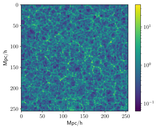
In this paper, we use 2D matter fields of 256256 pixels, which are generated as follows: First, for each realization we compute a 3D density field with voxels by assigning particle positions to the grid using the cloud-in-cell mass assignment scheme. Then we take a slice of and project to pixels by computing the average along the third axis. The resulting field represents a region with an area of 10001000 . The matter density fields are normalized to satisfy . In the following section, we study both the matter density field and its logarithm. Figure 3 provides an example of such a field.
We consider different cosmologies with five varying cosmological parameters: the matter density parameter , the baryon density parameter , the dimensionless Hubble parameter , the scalar spectral index , and finally , the average rms matter fluctuation smoothed at Mpc scale. We denote these parameters collectively as .
We use two different sets of simulations. The first set contains 15000 simulations of the Planck fiducial cosmology (Aghanim et al. 2018), for cosmological parameters (see Table 1). The second set of simulations is devised to numerically compute partial derivatives with respect to the five cosmological parameters. For each cosmological parameter , this set contains 1000 simulations for (i.e., 500 for each sign), the other parameters being held fixed at the fiducial values (see Villaescusa-Navarro et al. 2019 for more details). See Table 1 for the values of .
| Pk | Pk + Bk | WPH | P | P + B | WPH′ | |
|---|---|---|---|---|---|---|
| Size | 127 | 313 | 327 | 127 | 313 | 327 |
| 0.15 | 0.12 | 0.11 | 0.15 | 0.12 | 0.10 | |
| 0.16 | 0.12 | 0.075 | 0.12 | 0.097 | 0.064 | |
| 1.5 | 1.1 | 0.71 | 0.99 | 0.78 | 0.50 | |
| 0.74 | 0.52 | 0.20 | 0.25 | 0.20 | 0.11 | |
| 0.024 | 0.013 | 0.018 | 0.012 | 0.0097 | 0.0097 |
III.2 Fisher matrix analysis
For a given set of statistics, we can quantify the information that they contain (on average) with respect to the cosmological parameters by computing the Fisher information matrix of the parameters. Specifically, consider a set of scalar statistics (such as WPH moments) computed from a realization of the field. We denote by the expected value of , and by the covariance of and when is drawn under . If the statistics are jointly Gaussian and their covariance matrix does not depend on , the Fisher information matrix boils down to (Tegmark et al. 1997)
| (9) |
From this Fisher matrix we can compute the Cramér-Rao bound, which gives the asymptotically lowest possible variance for any unbiased estimator of based on :
| (10) |
In this paper, we numerically estimate the Fisher matrices (for each set of summary statistics considered) for the cosmological parameters corresponding to the Planck fiducial cosmology. We estimate the covariance matrices from the 15000 fiducial Planck simulations, while each partial derivative appearing in Eq. (9) is evaluated with the two sets of 500 simulations at . We checked the convergence of these estimates by verifying that the Cramér-Rao bounds changed only at the percent level when using 10000 (350) simulations to compute the covariance matrices (partial derivatives).
| WPH | + Pk | + Bk | WPH′ | + P | + B | |
|---|---|---|---|---|---|---|
| Size | 327 | 454 | 513 | 327 | 454 | 513 |
| 0.11 | 0.11 | 0.10 | 0.102 | 0.096 | 0.094 | |
| 0.075 | 0.073 | 0.070 | 0.064 | 0.063 | 0.062 | |
| 0.71 | 0.68 | 0.65 | 0.50 | 0.50 | 0.48 | |
| 0.20 | 0.20 | 0.19 | 0.11 | 0.11 | 0.11 | |
| 0.018 | 0.018 | 0.0095 | 0.0097 | 0.0096 | 0.0086 |

III.3 Fisher matrix results
We compare in this section the results obtained with three sets of summary statistics: the standard isotropic power spectrum (Pk), the power spectrum plus a set of isotropic bispectrum triangles (Pk + Bk), and a set of WPH statistics. Appendix A.3 describes the bispectrum triangle ensemble, which contains flattened, squeezed, and equilateral triangles. The WPH statistics are constructed from the WPH moments given in Eq. (8), which are invariant under rotations and parity. Appendix B.2 provides a complete description of these moments, which characterize all the scales of the image with 327 coefficients. A plot of a subset of moments from these WPH statistics are given in Fig. 9, and their covariance in Fig. 10. Note however that these figures use notations introduced in Sec. V.
For each of these descriptors, we evaluated the posterior distributions of the cosmological parameters obtained using the matter density field and its logarithm from the Quijote simulations. We expect the logarithm to make the density field more Gaussian, while transferring information from high-order correlations to the power spectrum (Neyrinck et al. 2009; Neyrinck et al. 2011; Neyrinck 2011). See Massara et al. 2020 for a similar case of a nonlinear transform applied to Quijote simulations.
Table 2 and Fig. 4 respectively show the marginal and full posterior distributions of cosmological parameters obtained with the Fìsher analysis. For all five cosmological parameters, the WPH statistics contain more information than the power spectrum. The improvement of forecast errors ranges from to a factor larger than 3. The relative improvement is generally larger for the matter density field than for its logarithm. This may be because the logarithm of the field is more Gaussian and the power spectrum suffices to characterize a Gaussian stationary field.
Compared to the power spectrum plus bispectrum, the WPH statistics provide better constraints on four of the cosmological parameters, the exception being . For those four parameters, the absolute improvement from Pk + Bk to WPH is similar to the improvement from Pk alone to Pk + Bk.
Table 3 shows the Fisher information results for joint WPH + Pk and WPH + Bk statistics. Except for with WPH + Bk statistics, only limited additional information is gained by adding these statistics to those built solely on WPH moments.

Numerous works (Byun et al. 2017, e.g.,) study the LSS field using the power spectrum together with bispectrum. For instance, Sefusatti et al. 2006b; Yankelevich and Porciani 2019; Chudaykin and Ivanov 2019 provide bispectrum forecasts for full sets of cosmological parameters. In particular, Hahn et al. 2019 computes from the N-body Quijote simulations the full information content of the redshift-space halo bispectrum for six cosmological parameters. However, the particular two-dimensional projected matter density field that we use here makes it difficult to quantitatively compare our results with those obtained in these earlier works. Reference Coulton et al. 2019 performs a similar analysis for weak-lensing surveys. They show the improvements gained by adding the bispectrum to the power spectrum and obtain results similar to our results for Pk and Pk + Bk. Given the widespread use of the bispectrum in cosmological parameter inference, current bispectrum results can be taken as a generic benchmark. Thus, we claim that the results obtained with WPH statistics compare favorably to state-of-the-art results obtained with these other summary statistics. A more quantitative comparison is deferred to later work, since it requires WPH statistics to be extended to 3D fields.
IV Statistical syntheses with WPH statistics
In this section, we show that WPH statistics embed a wide range of summary statistics commonly used in cosmology. For that purpose, we estimate WPH statistics on a subset of Quijote simulation maps, and generate from them synthetic maps based on a microcanonical maximum entropy principle. Then we compare these statistical syntheses to the whole sample of Quijote maps, using as summary statistics the power spectrum, bispectrum, probability density function (PDF), and Minkowski functionals.
Previous studies have considered similar syntheses based on either WPH statistics (Zhang and Mallat 2019; Villaescusa-Navarro et al. 2019) or the related Wavelet Scattering Transform (Mallat 2012; Bruna and Mallat 2013; Allys et al. 2019), but they reported only qualitative assessments, mostly from visual inspection. In contrast, in Sect. IV.2 below we report much more stringent quantitative tests based on a wide set of statistics commonly used in astrophysics.
IV.1 Microcanonical maximum entropy model
In this section we outline our generative algorithm for drawing sample realizations of a microcanonical maximum entropy model. A maximum entropy model is a probability distribution that satisfies a set of statistical constraints, while being as general as possible otherwise. This means that it maximizes the Shannon entropy . In this paper, we consider microcanonical models, which are defined as follows. Let denote a realization of the process under study and let be a set of statistics computed on this realization. We define the microcanonical set of width conditioned by as
| (11) |
where is a measure of the discrepancy between and . The microcanonical maximum entropy model is the model of maximal entropy defined over . This implies that it has a probability distribution that is uniform on . See Bruna and Mallat 2018 and Zhang and Mallat 2019 for the exact definition of and further explanation.
We could sample from microcanonical maximum entropy models with Monte-Carlo techniques, but such methods tend to be quite computationally expensive for a large number of statistical constraints (Lustig 1998). We therefore rely on a different approach, introduced in (Bruna and Mallat 2018). To produce one realization of the microcanonical model, we start from a realization of an homogeneous and isotropic Gaussian field which is then modified iteratively by gradient descent with respect to the loss function . Care must be taken that the descent preserves the key symmetries of the starting point: homogeneity and isotropy.
For this paper, we implement the microcanonical maximum entropy sampling in Python using the PyTorch library Paszke et al. 2017 to compute the gradient of the loss and we perform the loss descent using the L-BFGS-B Byrd et al. 1995 implementation of Scipy Virtanen et al. 2020.
IV.2 Statistical validation of the syntheses
We now assess the quality of the syntheses generated by the maximal entropy model. Rather than working with the matter density field itself, we chose to work with its logarithm. As the matter density field roughly follows a log-normal distribution, the distribution of its logarithm should be well approximated by a normal distribution. Indeed, we found that it was better reproduced by our maximal entropy model. We refer to Appendix C for further explanations on this choice.
The WPH statistics used in this section, and detailed in Appendix B.3, contain 6676 coefficients, significantly more than the 327 coefficients used for Fisher analysis in Sec. III. The increase occurs because the WPH moments used here are not invariant under rotations: they are constructed from Eq. (6) rather than from the isotropized version (8). We found that this choice led to better syntheses: even though syntheses based on isotropic moments (8) are visually indistinguishable from syntheses based on anisotropic moments (6), the various validation statistics presented below are better reproduced with anisotropic moments. This is likely due to the Cartesian grid breaking the rotational symmetry, especially at small scales. The other difference from the statistics of Sec. III is that here we use low-pass filters rather than WPH moments to constrain the scales at .
As sketched in section IV.1, the principle of the synthesis of a map is to adjust its pixels in order for its WPH moments to match those estimated from Quijote simulations. However, something slightly different is implemented in practice so some details are in order. Regarding the target WPH moments, they are collected in a vector obtained by averaging (a sample version of) Eq. (6) over a set of Quijote maps with periodic boundary conditions. Each Quijote map has a surface area of 1 (Gpc/)2 and is sampled on a grid of pixels. We found empirically that a set of maps was large enough to estimate the WPH coefficients up to with an accuracy sufficient for our purposes. We could have used a larger training set but we restrained ourselves to in order to illustrate that our method performs well with a small number of examples.
Regarding the synthesis process itself, maps are not produced individually but in batches of maps. We start from maps of size obtained as independent Gaussian white noise realizations. Then, their pixel values are adjusted by minimizing the joint loss
| (12) |
rather than minimizing the individual loss independently for each map . The motivation for this variant is that criterion (12) demands that the WPH statistics be matched on average over maps rather than for every map, thereby allowing some variability in the synthesis55 5 Such a variability is needed at large scales which have much fewer degrees of freedom. This issue will be the subject of future research. In this paper, we chose because it worked well in our syntheses and also because it was the practical upper limit imposed by the size of GPU memory. For our experiments, we ran 10 optimizations of (12) using the same , hence producing synthetic maps, taking about 50 GPU hours66 6 The GPU used was a GPU Nvidia Tesla P100 with 16Go of RAM.. Fig. 5-a,b shows one Quijote map and one synthesized map.

To assess the quality of the syntheses, we performed a variety of statistical analyses, comparing the 300 synthetic maps to an independent sample of 300 Quijote maps. In particular, we computed several -point statistics for up to 4 on both these sets of maps. We compared the pixel distributions (), power spectra (), bispectra (), and the standard deviation and correlation matrix of the empirical power spectrum (). We also computed three Minkowski functionals (MFs) for both sets of 300 maps. Figs. 5, 6, and 7 present these results.
For isotropic homogeneous fields, the bispectrum is defined by three wave-vectors satisfying the triangle inequalities, and therefore representing the lengths of the edges of a triangle. We focus on three configurations: squeezed triangles ( and ), flattened triangles (), and equilateral triangles (). Fig. 5-f,g shows the results for flattened and squeezed triangles and Fig. 6 those for equilateral triangles. Appendix A.3 describes the bispectrum computation in greater detail.
Minkowski functionals are statistics capturing the topology of the level sets of the field. They are used in cosmology to probe the non-Gaussianity of the CMB (Ade et al. 2014), to probe departures from General Relativity of the LSS (Fang et al. 2017), and to study lensing convergence maps (Parroni et al. 2020). In dimensions, there are three MFs that depend on a threshold , denoted , and . Their definitions are recalled in appendix A.4. The MFs of the sets of maps are shown in figure 7-b.

The results of these comparisons show that the syntheses from WPH statistics presented in this section perform remarkably well in reproducing the statistical properties of the logarithm of the Quijote LSS matter density field. Indeed, our syntheses reproduce the mean of the empirical power spectrum, its standard deviation, and its correlation within , , and , respectively. They also reproduce the squeezed and flattened bispectra within and , respectively, at spatial frequencies higher than , and within below this spatial frequency. The whole pixel PDF is also very well reproduced, including the tails down to 4 orders of magnitude below the peak. There is no particular discrepancy between the synthetic and the Quijote distributions of the empirical power spectrum, as shown in Fig. 7 at three arbitrary frequencies. Finally, the syntheses reproduce the three MFs to within , , and , respectively.
Note that the syntheses do not accurately reproduce the equilateral bispectrum (Fig. 6), although they do capture its general shape and changes of sign. This result may be related to the fact that equilateral bispectrum configurations correspond to correlations between three clearly separate frequencies, . Thus moments built from convolutions of only two wavelets cannot directly characterize them. Extending the WPH construction to characterize such couplings is left to future work.
Previous works have used convolutional neural networks, and especially GANs, to produce syntheses of astrophysical fields. For example, Ramanah et al. 2020 uses a GAN to emulate accurate high-resolution features from computationally cheaper low-resolution cosmological simulations. Similarly, in Aylor et al. 2019, the authors use GANs to generate maps representing the interstellar medium. More recently, Tamosiunas et al. 2020 trained GANs to reproduce both weak lensing convergence maps and dark matter over-density fields. All these works assess the quality of the syntheses as in the present paper, i.e., by computing histograms, power spectra, bispectra, and Minkowski functionals. Our results are of similar quality to these earlier works.
However, because our method relies on explicit construction of statistics, it is not subject to the usual caveats of neural network methods. First of all, the WPH statistics can be physically interpreted (see Sec. V). Secondly, neural network methods must learn a large number of parameters (weights) from a huge training dataset, whereas we used only Quijote maps for our syntheses. Also, the use of GANs to generate new realizations of a given process can suffer from mode collapse, i.e., the omission of certain object classes in the generated images and loss of the associated statistical features (Bau et al. 2019). These points underline the advantages of maximum entropy syntheses built with a suitably tailored statistical description such as the WPH moments.
V Physical interpretation of the WPH statistics
This section discusses the physical meaning of the various WPH moments and their relation to other summary statistics. It complements the discussion of symmetries of Sec. II.4. See also Appendix B for the full specification of the WPH statistics.
To identify the physical properties encoded in the WPH moments, we organize the moments into five categories. We define each category by selecting a set of parameters. The first three categories contain moments that each have only a single spectral wavelet band (i.e., ; see Sec. V.1 below), while the other two contain moments describing a coupling between two wavelet bands of central frequencies and (see Sec. V.2).
To study these different categories of moments, we progressively include them in our analysis, and build five nested sets of statistics that we call model I to model V. While model I merely contains power spectrum information, model V corresponds to the WPH statistics used in Sec. III and IV. Using each of these models, we compute the Fisher information for the Quijote simulated LSS matter density field and also for , and perform statistical syntheses of .

V.1 Terms related to a single wavelet frequency band
Let us first consider WPH moments that describe a single spectral wavelet band. Thus we start from the moments given in Eq. (6), and restrict to cases where . Hence, we focus on moments of the form
| (13) |
and we consider three such terms obtained by taking the phase exponents equal to , , or . Explicitly, these are
| (14) | ||||
| (15) | ||||
| (16) |
Note that corresponds to the covariance of wavelet transforms presented in Sec. II.2.
Model I: moments; power spectrum.
As shown in Sec. II.2, the moments, which form model I WPH statistics, only depend on the power spectrum of . Thus we see that syntheses from model I generate fields close to Gaussian (see Fig. 8). These fields have in particular a Gaussian PDF (see Fig. 11) and the ensemble mean of their bispectra is null.
With these moments we can also see the impact on the spectral resolution of the number of relative spatial translations used (see Eq. 33 of Appendix B). Figure 12 illustrates this property by showing the power spectrum of the model I syntheses for two cases: The imprints of the wavelet spectral bands are clearly visible when no translations are used (i.e., only, which corresponds to ), while they are reduced when (i.e., two nonzero translations in each direction). We obtained similar results for the Fisher analysis of cosmological parameters. Indeed, the amount of information on cosmological parameters carried by model I WPH statistics increases with the number of retained values of , eventually converging to the information contained in the standard power spectrum.

Model II: moments and sparsity.
We build model II by adding the moments to model I. These moments allow us to quantify the ratio between the and norms of the wavelet transform of . This ratio characterizes the sparsity of the field in the wavelet basis (see Zhang and Mallat 2019, for a more detailed discussion). In the Quijote LSS simulations, these coefficients indicate that the small scales are sparser than the large ones, and as the scale increases the sparsity converges to that of a Gaussian field, see Fig. 9. We expect such a result, since the LSS density fields are expected to become Gaussian at scales larger than 100 Mpc (about 25 pixels in our maps).
The amount of Fisher information with respect to the cosmological parameters is significantly higher in model II than in model I, as shown by Fig. 8-a,b. Similarly to model I, increasing the number of spatial shifts in model II substantially improves the Fisher information with respect to the cosmological parameters.
The moments do not substantially improve the synthesis results, as can be seen in the maps in Fig. 8.
Model III: moments and first structures.
To build the third model of WPH statistics, we add the moments to model II. These moments measure a covariance between wavelet coefficients that undergo two different operations (namely, modulus and identity). Hence they mainly describe couplings between different spatial frequencies within a single wavelet band, see Sec. II.3. Thus, they probe the impact of the interaction between neighboring scales.
The moments significantly improve the syntheses generated. The model III map in Fig. 8 illustrates this, where the familiar foamy structure of the LSS is recognized. In Fig. 11 we see that model III (unlike models I and II) reproduces the main shape of the PDF of the Quijote simulations. Similarly, the model III syntheses reproduce the Minkowski functionals and the flattened bispectrum, but not the squeezed bispectrum. This last result is due to the fact that squeezed bispectrum triangles characterize the joint information between Fourier modes of wave-vectors of very different sizes.
In spite of these results, model III makes only minor improvements to the Fisher information regarding cosmological parameters. This is especially noticeable for the LSS matter density field (Fig. 8a), and less so for its logarithm (Fig. 8b). These results emphasize that although the interactions between nearby scales are important statistics for qualitatively reproducing the web structure of the LSS, they do not seem efficient for discriminating between different cosmological parameter values.
V.2 Couplings between wavelet frequency bands
The second type of moment that we consider characterizes couplings between two wavelet spectral bands with central spatial frequencies and . We consider three kinds of such couplings based on the moments , with different values of . In each case, the two phase harmonics of wavelet transforms contain common spatial frequencies of oscillation. For each term, we set (corresponding to spatial scales ), without loss of generality. Similarly to the definition of Eq. (13), we define
| (17) |
For the first two types of moment, we consider and . Explicitly, those are
| (18) | ||||
| (19) |
For , the and moments are identical to and defined in the previous section. Note that is not symmetric under exchange of and , but it is negligibly small when , as discussed below.
These moments can be interpreted as follows. First, quantifies the correlation between local levels of oscillations at and spatial frequencies. Then, evaluates the correlation between the amplitude of the local level of oscillation at the frequency and the oscillation at the frequency. For this second moment, since is filtered at a wavelength, it is clear that the correlation of its amplitude with a term gives a negligible result if this second convolution oscillates at a characteristic scale .
Our last coupling uses . We define
| (20) | |||||
For , this moment is equivalent to . The computation of such WPH moments is illustrated in Fig. 3 and was discussed in Sec. II.3. Computed from fields filtered at different scales which are made synchronous, such terms are designed to characterize the relative phase shift between different scales.
These three coupling terms can also be understood from a Fourier space point of view. For each of them, Fig. 13 illustrates how the phase harmonics operator modifies the spectral support of the field convolved with the and wavelets. The three coupling terms correspond to different ways of achieving a (possibly partial) spectral overlap by band-passing followed by the phase operation.
Models IV & V: couplings between different wavelet bands.
We define model IV by adding the and moments to model III. Finally, we define Model V by adding the moments. Note that these models include terms for which and have the same norm but different orientations. Model V corresponds to the statistical descriptions used in Sec. III and IV.
The syntheses generated from model IV are significantly better than those of model III. This model reproduces the squeezed bispectrum triangles, as well as the tails of the PDF (with results that are better than model III by a factor close to 5). This result underlines that and moments are related to couplings between scales that are far apart. In particular, the PDF result exhibits how the precise distribution of peaks of the LSS seems to be related to couplings between different scales that sum up together in a coherent way. By contrast, model V does not significantly improve the syntheses compared to model IV.
For cosmological parameter inference, Fig. 8 shows how both models IV and V noticeably improve the forecast errors. These improvements are generally significantly larger than those obtained with the local coupling added in model III. It is interesting to see that while the moments play only a minor role in reproducing the standard statistics in syntheses, they do contain a substantial amount of information about cosmological parameters. This result could indicate that the moments are not directly related to the summary statistics we used to validate the syntheses.
Importance of the ratio between coupled scales.
For a given set of WPH statistics, the value quantifies the maximum scale difference being characterized by the moments. Indeed, the maximum ratio between such scales is . Similarly, the ratio between the norm of the more distant spatial frequencies that are coupled is .
For nonlinear physical processes, this parameter is of major importance. Indeed, nonlinearity implies a statistical interaction between different scales. The more nonlinear a given process is, the stronger we expect distant scales to be coupled (Bruna et al. 2015). We also expect different nonlinear couplings to have distinct signatures in the way scales decouple from one another when the ratio between scales increases.
Let us illustrate the importance of . For cosmological parameter inference, one can compute how the Fisher forecast errors evolve for model V as we increase from 0 (which corresponds to model III). As shown in Fig. 14, we find that significant information is contained in the coupling between different scales. The Fisher results keep improving even when we add terms with , representing coupling between scales that are very far apart (e.g., 2 and 64 pixels). This especially contrasts with the minor improvements brought about by the inclusion of couplings between nearby scales.
The increase of the Fisher information with is different for each cosmological parameter. In particular, this improvement is only modest for , and especially small for above . Note that and are the two parameters for which the WPH statistics do not characterize much more information than the power spectrum (see Table 2). This indicates that these particular parameters do not especially impact the way distant scales couple. This result seems rather natural for , since it is merely a normalization of the matter fluctuation power spectrum.
The importance of also appears for the syntheses. Even though the cosmic web structure visually appears with a model where (see the model III map in Fig. 8), larger values of are needed to properly reproduce the tails of the PDF, which for instance characterize the distribution of peaks of the LSS. This can be seen by carefully comparing tails of the model III, IV, and V results in Fig. 11. Similarly, larger values of must be included to reproduce the squeezed triangle bispectrum of the Quijote LSS field (see Fig. 15). This result is, however, completely to be expected, since those triangles characterize couplings between very different scales.
VI Conclusion
In this paper, we introduced low-dimensional Wavelet Phase Harmonics (WPH) statistics to analyze and synthesize two-dimensional matter density fields from the Quijote LSS simulations. We built the WPH statistics from WPH moments, which were recently introduced in data science. The WPH moments correspond to the covariance of wavelet coefficients whose spatial frequencies are made synchronous by means of a nonlinear operator called the phase harmonic operator.
The main result of this paper is the construction of specific low-dimensional WPH statistics that achieve state-of-the-art results for both capturing cosmological information and producing statistical syntheses. We obtained these results by computing the Fisher information of these statistics with respect to five cosmological parameters, and by producing maximum-entropy syntheses that were validated by means of classic summary statistics. To our knowledge, it is the first time that state-of-the-art results have been obtained for both of these tasks from the same statistical description. We also illustrated the interpretability of WPH statistics by discussing the types of information described by distinct subsets of WPH moments.
In this paper, we applied the WPH statistics to the projected LSS matter density field. However, their construction is not specific to this process, and they can therefore be used to study other non-Gaussian physical fields. A natural extension is to apply this method to three-dimensional fields, which is left for future work. This would allow a direct comparison with results obtained from other summary statistics or from machine learning methods.
The quality of the statistical syntheses produced in this paper validates the relevance of using WPH statistics to study the LSS. Moreover, this work shows that WPH statistics can serve as a generative model for non-Gaussian fields. They could be used to generate mock syntheses, or to perform data augmentation for machine learning purposes. The syntheses can be performed from a limited training set (here, we used 30 Quijote maps), and therefore we could train our model directly on observational data.
Acknowledgments
We thank D. Spergel, B. Ménard, and B. Wandelt, for fruitful discussions, as well as F. Levrier and B. Régaldo-Saint Blancard for their comments on the draft. We also thank G. P. Collins for his valuable assistance in the preparation of this document, as well as the anonymous referee, whose comments helped to clarify the paper. EA thanks the Flatiron Institute of the Simons Foundation for its generous hospitality during the preparation of this work. FVN acknowledges funding from the WFIRST program through NNG26PJ30C and NNN12AA01C. SM also acknowledges support from the PRAIRIE 3IA Institute of the French ANR-19-P3IA-0001 program.
Appendix A Mathematical specifications
A.1 Bump steerable mother wavelet
The multiscale bump steerable wavelets used for the wavelet transform described in Sec. II.1 are built from a mother wavelet . Following Mallat et al. 2018, which first introduced bump steerable wavelets, we define via its Fourier transform as
| (21) |
where is the central frequency of the wavelet, is a normalization constant, is the number of angles used in the multiscale wavelet family, and is the indicator function that returns 1 if and 0 otherwise. Following Zhang and Mallat 2019, we use , and with .
A.2 Scaling functions
We also consider convolutions of the field with a family of low-pass filters called scaling functions. These low-pass filters are built from an initial Gaussian window defined as
| (22) |
The individual are obtained from by dilations of :
| (23) | ||||
| (24) |
Again following Zhang and Mallat 2019, we use .
A.3 Bispectrum estimates
For our bispectrum computations, we have adapted the method described in Jung et al. 2018 by which a smoothed isotropic bispectrum is estimated as a 3-point correlation between three filtered versions of the field. Specifically, we use isotropic filters which select only frequencies such that , and we define . The bispectrum is then estimated from . In particular, we use
| (25) |
We define as a reference value for wavenumbers, and we use in Eq. (25) for the bispectrum computations used to validate the syntheses in Sec. IV.
In Sec. III, we use , and we specify the following set of bispectrum statistics to compute Fisher information about cosmological parameters:
- •
All flattened triangle configurations , with for between 1 and 62.
- •
All equilateral triangle configurations , with for between 1 and 62.
- •
All squeezed triangle configurations , with for between 1 and 62, and .
This set contains 62 triangles of each type, for a total of 186 bispectrum terms.
A.4 Minkowski functionals
We use three Minkowski functionals (, , ) to assess the quality of the syntheses in section IV.2. Given a threshold , these are respectively the area, the perimeter, and the genus defined by the threshold. More precisely, for a field defined on an area , let us define and similarly for and . Let be the area of , its perimeter, and () the number of connected components of (). Then:
| (26) |
Appendix B Specifications of WPH models
B.1 WPH Statistics
We build the specific WPH statistics used in this paper for Fisher analysis and statistical syntheses from two types of WPH moments: moments describing a single wavelet frequency band and moments describing two. Both are built from the basic WPH moments discussed in Sec. II.3 and defined by Eq. (6), which we repeat here for reference:
| (6) |
where are wavelet frequencies, denotes the th phase harmonic as defined in Eq. (5), and is a spatial shift.
The moments used for our statistics are:
| (27) | ||||
| (28) | ||||
| (29) |
Specifically, we use moments , , , , , and , and we restrict to . The physical significance and motivation for using these moments is discussed in Sec. V.
We also define WPH moments and that are invariant under rotation and parity, based on the invariant WPH moments discussed in Sec. II.4,
| (8) |
where is an absolute angle, denotes an angular average (over and ), and the moment refers to the standard WPH moment of Eq. (6) with the and indices related by Eq. (2) in the usual way. Specifically, the invariant moments for our statistics are:
| (30) | ||||
| (31) | ||||
| (32) |
with the restriction .
To construct these statistics, we consider only a discrete set of spatial translations labeled by an integer and an angle . Translation is defined with respect to the wavelet of largest characteristic wavelength appearing in Eq. (6), and is oriented at an angle relative to the direction of oscillation of this wavelet:
| (33) |
where is the unit vector in the specified direction. We use integer values ranging from 0 to , with various choices of depending on the specific type of moment and the values of . For the invariant (isopar) statistics, we use . Otherwise we restrict to integer multiples of . Note that these translations are redundant when larger than half of the size of the fields (128 pixels in this paper).
B.2 Models for Fisher analysis
| Model | I | II | III | IV | V |
|---|---|---|---|---|---|
| Moments | + | + | + , | + | |
| Total size | 32 | 64 | 96 | 252 | 327 |
We present in this section the WPH statistics used for the Fisher analysis of Secs. III and V. These statistics have integer values from 0 and 7, corresponding to wavelengths from 2 to 256 pixels. Thus, all the scales of the matter density fields are characterized with WPH moments. These WPH statistics are also invariant under rotation and parity, and characterize couplings between all wavelet bands, with . They are defined as follows:
- •
For , , and moments, we consider all values from 0 to 7. For each value, we consider all possible translations with and , where .
- •
For , , and , we consider all pairs satisfying . For , we take only . For , we take when , and we take otherwise. Finally, we consider translations with if and , and no translations otherwise (i.e., we keep only). Note that moments with and are equal to moments and are therefore omitted to avoid double counting.
These WPH statistics contain a total of 327 WPH moments. In Sec. V, we divide these WPH statistics into a set of five nested models, model I to model V, to assess how the Fisher information about cosmological parameters increases as WPH moments with different properties and physical significance are included. These models are summarized in Table 4.
| Model | I | II | III | IV | V |
|---|---|---|---|---|---|
| Moments | + | + | + , | + , | |
| Total size | 677 | 1349 | 2021 | 5412 | 6676 |

B.3 Models for statistical syntheses
This section presents the WPH statistics used to perform syntheses in Sec. IV and V. The WPH statistics used in the syntheses of Sec. IV have integer values from 0 to 5, corresponding to wavelengths up to 64 pixels. They thus do not characterize in terms of WPH moments the largest scales of the matter density fields, but describe couplings between all scales up to , with . The moments used for these statistics are not required to be invariant under rotation and parity, contrary to those used for Fisher analysis. They are defined as follows:
- •
For , , and moments, we consider all values from 0 to 5 and values from to . For each value, we consider for and all possible translations with and . No translations are applied to .
- •
For , , and , we consider all pairs satisfying , and all values . We take for , and for and . For and , when , we apply all possible translations with and . No translations are applied (i.e., we take ) for when , or for with any . moments with and are omitted because they are equal to moments.
To complete these WPH statistics and better constrain the scales that are not probed by WPH moments as well as the probability density function, we also consider convolutions of the field with a family of low-pass filters called scaling functions, defined in Appendix A.2. We therefore added the following scaling moments to the WPH moments:
| (34) | ||||
| (35) |
with between and and , yielding 16 scaling moments.
Appendix C Limitations of the model and direct syntheses of the field
We applied the method presented in section IV to directly generate syntheses of the raw density field (instead of its logarithmic value). However, this field is strictly positive, with a wide dynamic range. The resulting syntheses did not reproduce the sharp constraint . An example of these syntheses and their histogram is provided in Fig.16. This figure, however, shows that the filamentary structure of the LSS density field is nevertheless recovered.
Another possibility to obtain strictly positive syntheses of the density field is to take the exponential of the syntheses of presented in section IV. The histograms and the Minkowski functionals of the resulting syntheses reproduce the statistics of the simulations with an accuracy similar to the results presented in IV.2. However, the other statistics are not well recovered. For example, the mean and the standard deviation of the power spectrum of the syntheses differ from those of the simulations by respectively and for most of the spatial frequency .
References
- Sefusatti et al. (2006a) E. Sefusatti, M. Crocce, S. Pueblas, and R. Scoccimarro, Cosmology and the bispectrum, Phys. Rev. D74, 023522 (2006a), arXiv:astro-ph/0604505 [astro-ph] .
- Byun et al. (2017) J. Byun, A. Eggemeier, D. Regan, D. Seery, and R. E. Smith, Towards optimal cosmological parameter recovery from compressed bispectrum statistics, Mon. Not. Roy. Astron. Soc. 471, 1581 (2017), arXiv:1705.04392 [astro-ph.CO] .
- Hahn et al. (2019) C. Hahn, V.-N. Francisco, C. Emanuele, and S. Roman, Constraining with the bispectrum i: Breaking parameter degeneracies, arXiv preprint arXiv:1909.11107 (2019).
- Chiang et al. (2014) C.-T. Chiang, C. Wagner, F. Schmidt, and E. Komatsu, Position-dependent power spectrum of the large-scale structure: a novel method to measure the squeezed-limit bispectrum, JCAP 1405, 048, arXiv:1403.3411 [astro-ph.CO] .
- Stuart et al. (1963) A. Stuart, M. G. Kendall, et al., The advanced theory of statistics (Griffin, 1963).
- Obreschkow et al. (2013) D. Obreschkow, C. Power, M. Bruderer, and C. Bonvin, A robust measure of cosmic structure beyond the power-spectrum: Cosmic filaments and the temperature of dark matter, Astrophys. J. 762, 115 (2013), arXiv:1211.5213 [astro-ph.CO] .
- Wolstenhulme et al. (2015) R. Wolstenhulme, C. Bonvin, and D. Obreschkow, Three-point phase correlations: a new measure of nonlinear large-scale structure, Astrophys. J. 804, 132 (2015), arXiv:1409.3007 [astro-ph.CO] .
- Alpaslan et al. (2014) M. Alpaslan et al., Galaxy and mass assembly (gama): Fine filaments of galaxies detected within voids, Mon. Not. Roy. Astron. Soc. 440, L106 (2014), arXiv:1401.7331 [astro-ph.CO] .
- Ali et al. (2018) K. Ali, D. Obreschkow, C. Howlett, C. Bonvin, C. Llinares, F. O. Franco, and C. Power, Cosmological constraints from fourier phase statistics, Mon. Not. Roy. Astron. Soc. 479, 2743 (2018), arXiv:1806.10276 [astro-ph.CO] .
- Bardeen et al. (1985) J. M. Bardeen, A. Szalay, N. Kaiser, and J. Bond, The statistics of peaks of gaussian random fields, Astrophys. J. 304, 15 (1985).
- Pisani et al. (2019) A. Pisani, E. Massara, D. N. Spergel, D. Alonso, T. Baker, Y.-C. Cai, M. Cautun, C. Davies, V. Demchenko, O. Doré, et al., Cosmic voids: a novel probe to shed light on our universe, arXiv preprint arXiv:1903.05161 (2019).
- Cohen and Ryan (1995) A. Cohen and R. D. Ryan, Wavelets and multiscale signal processing (Springer, 1995).
- Mallat (1999) S. Mallat, A wavelet tour of signal processing (Elsevier, 1999).
- Van Den Berg (2004) J. Van Den Berg, Wavelets in physics (Cambridge University Press, 2004).
- Farge et al. (2010) M. Farge, K. Schneider, O. Pannekoucke, et al., Multiscale representations: fractals, self-similar random processes and wavelets, Handbook of Environmental Fluid Dynamics 2, 311 (2010).
- Farge and Schneider (2015) M. Farge and K. Schneider, Wavelet transforms and their applications to mhd and plasma turbulence: a review, Journal of Plasma Physics 81 (2015).
- Flandrin (1992) P. Flandrin, Wavelet analysis and synthesis of fractional brownian motion, IEEE Transactions on information theory 38, 910 (1992).
- Meyer et al. (1999) Y. Meyer, F. Sellan, and M. S. Taqqu, Wavelets, generalized white noise and fractional integration: the synthesis of fractional brownian motion, Journal of Fourier Analysis and Applications 5, 465 (1999).
- Mallat et al. (2018) S. Mallat, S. Zhang, and G. Rochette, Phase harmonic correlations and convolutional neural networks, arXiv preprint arXiv:1810.12136 (2018).
- Zhang and Mallat (2019) S. Zhang and S. Mallat, Maximum entropy models from phase harmonic covariances, arXiv preprint arXiv:1911.10017 (2019).
- Zarka et al. (2019) J. Zarka, L. Thiry, T. Angles, and S. Mallat, Deep network classification by scattering and homotopy dictionary learning, arXiv preprint arXiv:1910.03561 (2019).
- Cheng et al. (2020) S. Cheng, Y.-S. Ting, B. Ménard, and J. Bruna, A new approach to observational cosmology using the scattering transform, arXiv preprint arXiv:2006.08561 (2020).
- Villaescusa-Navarro et al. (2019) F. Villaescusa-Navarro, C. Hahn, E. Massara, A. Banerjee, A. M. Delgado, D. K. Ramanah, T. Charnock, E. Giusarma, Y. Li, E. Allys, et al., The quijote simulations, arXiv preprint arXiv:1909.05273 (2019).
- Lewis et al. (2000) A. Lewis, A. Challinor, and A. Lasenby, Efficient computation of CMB anisotropies in closed FRW models, Astrophys. J. 538, 473 (2000), arXiv:astro-ph/9911177 [astro-ph] .
- Springel (2005) V. Springel, The Cosmological simulation code GADGET-2, Mon. Not. Roy. Astron. Soc. 364, 1105 (2005), arXiv:astro-ph/0505010 [astro-ph] .
- Aghanim et al. (2018) N. Aghanim, Y. Akrami, M. Ashdown, J. Aumont, C. Baccigalupi, M. Ballardini, A. Banday, R. Barreiro, N. Bartolo, S. Basak, et al., Planck 2018 results. vi. cosmological parameters, arXiv preprint arXiv:1807.06209 (2018).
- Tegmark et al. (1997) M. Tegmark, A. N. Taylor, and A. F. Heavens, Karhunen-loeve eigenvalue problems in cosmology: How should we tackle large data sets?, The Astrophysical Journal 480, 22 (1997).
- Neyrinck et al. (2009) M. C. Neyrinck, I. Szapudi, and A. S. Szalay, Rejuvenating the matter power spectrum: restoring information with a logarithmic density mapping, The Astrophysical Journal Letters 698, L90 (2009).
- Neyrinck et al. (2011) M. C. Neyrinck, I. Szapudi, and A. S. Szalay, Rejuvenating power spectra. ii. the gaussianized galaxy density field, The Astrophysical Journal 731, 116 (2011).
- Neyrinck (2011) M. C. Neyrinck, Rejuvenating the matter power spectrum. iii. the cosmology sensitivity of gaussianized power spectra, The Astrophysical Journal 742, 91 (2011).
- Massara et al. (2020) E. Massara, F. Villaescusa-Navarro, S. Ho, N. Dalal, and D. N. Spergel, Using the marked power spectrum to detect the signature of neutrinos in large-scale structure, arXiv preprint arXiv:2001.11024 (2020).
- Sefusatti et al. (2006b) E. Sefusatti, M. Crocce, S. Pueblas, and R. Scoccimarro, Cosmology and the bispectrum, Physical Review D 74, 023522 (2006b).
- Yankelevich and Porciani (2019) V. Yankelevich and C. Porciani, Cosmological information in the redshift-space bispectrum, Monthly Notices of the Royal Astronomical Society 483, 2078 (2019).
- Chudaykin and Ivanov (2019) A. Chudaykin and M. M. Ivanov, Measuring neutrino masses with large-scale structure: Euclid forecast with controlled theoretical error, Journal of Cosmology and Astroparticle Physics 2019 (11), 034.
- Coulton et al. (2019) W. R. Coulton, J. Liu, M. S. Madhavacheril, V. Böhm, and D. N. Spergel, Constraining neutrino mass with the tomographic weak lensing bispectrum, Journal of Cosmology and Astroparticle Physics 2019 (05), 043.
- Mallat (2012) S. Mallat, Group invariant scattering, Communications on Pure and Applied Mathematics 65, 1331 (2012), https://onlinelibrary.wiley.com/doi/pdf/10.1002/cpa.21413 .
- Bruna and Mallat (2013) J. Bruna and S. Mallat, Invariant scattering convolution networks, IEEE Transactions on Pattern Analysis and Machine Intelligence 35, 1872 (2013).
- Allys et al. (2019) E. Allys, F. Levrier, S. Zhang, C. Colling, B. Regaldo-Saint Blancard, F. Boulanger, P. Hennebelle, and S. Mallat, The rwst, a comprehensive statistical description of the non-gaussian structures in the ism, Astronomy & Astrophysics 629, A115 (2019).
- Bruna and Mallat (2018) J. Bruna and S. Mallat, Multiscale sparse microcanonical models, arXiv preprint arXiv:1801.02013 (2018).
- Lustig (1998) R. Lustig, Microcanonical monte carlo simulation of thermodynamic properties, The Journal of chemical physics 109, 8816 (1998).
- Paszke et al. (2017) A. Paszke, S. Gross, S. Chintala, G. Chanan, E. Yang, Z. DeVito, Z. Lin, A. Desmaison, L. Antiga, and A. Lerer, Automatic differentiation in pytorch, openreview.net (2017).
- Byrd et al. (1995) R. H. Byrd, P. Lu, J. Nocedal, and C. Zhu, A limited memory algorithm for bound constrained optimization, SIAM Journal on Scientific Computing 16, 1190 (1995), https://doi.org/10.1137/0916069 .
- Virtanen et al. (2020) P. Virtanen, R. Gommers, T. E. Oliphant, M. Haberland, T. Reddy, D. Cournapeau, E. Burovski, P. Peterson, W. Weckesser, J. Bright, S. J. van der Walt, M. Brett, J. Wilson, K. Jarrod Millman, N. Mayorov, A. R. J. Nelson, E. Jones, R. Kern, E. Larson, C. Carey, İ. Polat, Y. Feng, E. W. Moore, J. Vand erPlas, D. Laxalde, J. Perktold, R. Cimrman, I. Henriksen, E. A. Quintero, C. R. Harris, A. M. Archibald, A. H. Ribeiro, F. Pedregosa, P. van Mulbregt, and S. . . Contributors, SciPy 1.0: Fundamental Algorithms for Scientific Computing in Python, Nature Methods https://doi.org/10.1038/s41592-019-0686-2 (2020).
- Ade et al. (2014) P. A. R. Ade et al. (Planck), Planck 2013 results. xxiii. isotropy and statistics of the cmb, Astron. Astrophys. 571, A23 (2014), arXiv:1303.5083 [astro-ph.CO] .
- Fang et al. (2017) W. Fang, B. Li, and G.-B. Zhao, New probe of departures from general relativity using minkowski functionals, Phys. Rev. Lett. 118, 181301 (2017), arXiv:1704.02325 [astro-ph.CO] .
- Parroni et al. (2020) C. Parroni, V. F. Cardone, R. Maoli, and R. Scaramella, Going deep with minkowski functionals of convergence maps, Astron. Astrophys. 633, A71 (2020), arXiv:1911.06243 [astro-ph.CO] .
- Ramanah et al. (2020) D. K. Ramanah, T. Charnock, F. Villaescusa-Navarro, and B. D. Wandelt, Super-resolution emulator of cosmological simulations using deep physical models, arXiv preprint arXiv:2001.05519 (2020).
- Aylor et al. (2019) K. Aylor, M. Haq, L. Knox, Y. Hezaveh, and L. Perreault-Levasseur, Cleaning our own dust: Simulating and separating galactic dust foregrounds with neural networks, arXiv preprint arXiv:1909.06467 (2019).
- Tamosiunas et al. (2020) A. Tamosiunas, H. A. Winther, K. Koyama, D. J. Bacon, R. C. Nichol, and B. Mawdsley, Towards universal cosmological emulators with generative adversarial networks (2020), arXiv:2004.10223 .
- Bau et al. (2019) D. Bau, J.-Y. Zhu, J. Wulff, W. Peebles, H. Strobelt, B. Zhou, and A. Torralba, Seeing what a gan cannot generate, in Proceedings of the IEEE International Conference on Computer Vision (2019) pp. 4502–4511.
- Bruna et al. (2015) J. Bruna, S. Mallat, E. Bacry, J.-F. Muzy, et al., Intermittent process analysis with scattering moments, The Annals of Statistics 43, 323 (2015).
- Jung et al. (2018) G. Jung, B. Racine, and B. van Tent, The bispectra of galactic CMB foregrounds and their impact on primordial non-Gaussianity estimation, Journal of Cosmology and Astroparticle Physics 11, 047.