Extreme value theory for constrained physical systems
Abstract
We investigate extreme value theory for physical systems with a global conservation law which describe renewal processes, mass transport models and long-range interacting spin models. As shown previously, a special feature is that the distribution of the extreme value exhibits a non-analytical point in the middle of the support. We expose exact relationships between constrained extreme value theory and well-known quantities of the underlying stochastic dynamics, all valid beyond the midpoint in generality, i.e. even far from the thermodynamic limit. For example for renewal processes, the distribution of the maximum time between two renewal events is exactly related to the mean number of these events. In the thermodynamic limit, we show how our theory is suitable to describe typical and rare events which deviate from classical extreme value theory. For example for the renewal process, we unravel dual scaling of the extreme value distribution, pointing out two types of limiting laws: a normalisable scaling function for the typical statistics and a non-normalised state describing the rare events.
I Introduction
Extreme events are a large class of phenomena in natural and man-made systems which are uncommon compared to the usual dynamics bouchaud1997universality; albeverio2006extreme; embrechts2013modelling; fortin2015applications; fortin2015applications; MAJUMDAR20201. Despite their rare occurrence they still can have influential consequences, e.g. the fastest sperm in fertilization meerson2015mortality; schuss2019redundancy, the longest trapping time in transport wang2019transport and first passage problems in Markov processes hartich2019extreme. The original problem considers a set of independent and identically distributed (IID) random variables and describes the statistics of its maximum . Let be the probability density function (PDF) of the random variables and the cumulative distribution function (CDF). When the maximum has the value then all other random variables are less than or equal to . So the CDF of the maximum is and hence the PDF of the maximum is obviously
| (1) |
A central result of classical extreme value theory (EVT) is that the limiting maximum PDF for large converges to one of three classes of distributions called Weibull, Gumbel or Fréchet depending on the large behaviour of when is shifted and rescaled appropriately embrechts2013modelling; zarfaty2020accurately; gumbel2012statistics; fisher1928limiting. However, for most systems the assumption of IID random variables has to be abandoned.
Recently EVT was studied for a wide range of different models whose common property is the global confinement of their dynamics, see MAJUMDAR20201 for a review. This global conservation induces correlations among the random variables. It is a common trait shared in many models including renewal processes (RP) godreche2001statistics; niemann2016renewal; wang2018renewal; feller1971introduction; lowen1993fractal, mass transport models such as zero range processes (ZRP) evans2006canonical; majumdar2010real; majumdar2005nature; zia2004construction; evans2005nonequilibrium, and long-range interacting spin models such as the truncated inverse distance squared Ising model (TIDSI) bar2014mixed; bar2014mixed2. These three models describe numerous physical systems, including zero crossing of Brownian motion, arrival times at a detector, interacting systems to name only a few.
Particular attention was devoted to systems which loosely speaking are scale free, such as fractal renewal theory with diverging mean waiting time and diverging variance of the waiting time (see below). These systems exhibit large fluctuations and dominance of the extreme. It was shown previously how the global constraint may modify completely the classical EVT in the sense of strong deviations from Fréchet’s law. Somewhat similar to the classical ensembles of statistical physics, e.g. microcanonical ensembles with fixed
energy, volume and number of particles and canonical ensembles where the temperature of the bath is the constrain, the different constraints discussed below also give rich physical behaviours specific to the ensemble/model. For each model there are several classes of limiting laws in the thermodynamic limit when the global constraint diverges. These classes depend on the model parameters and were studied for RP godreche2009longest; godreche2014universal; godreche2015statistics; vezzani2019single; wang2019transport; scheffer1995rank, ZRP majumdar2010real; evans2008condensation and TIDSI bar2016exact. For example for RP with fat-tailed waiting times, typical fluctuations of the maximum go through a dynamical phase transition depending on the existence or non-existence of the mean waiting time. When the mean exists Fréchet’s law holds typically, when it doesn’t exist the behaviour is completely different godreche2015statistics. A similar situation exists for TIDSI in the critical phase between ferromagnetic and paramagnetic phase bar2016exact; godreche2017longestaa. However, a particular limiting law might reflect only part of the truth. So does Fréchet’s law predict a diverging second moment of the largest waiting time in a renewal process. However, that is impossible since all waiting times are shorter than the observation time. This does not imply that Fréchet’s law is incorrect, only that it must be modified in its tail. To put differently, the constraint yields a natural cut off and this modifies the description of classical EVT vezzani2019single; wang2019transport. In below main text, we discuss the thermodynamic limit for each model and how our results help to classify limiting behaviours.
Our work addresses two main themes. First without restoring to a thermodynamic limit, we provide complete set of relations between constrained EVT and much simpler quantifiers of the underlying stochastic dynamics. These exact relations are valid for any value of the global constraint, i.e. close to and far from the thermodynamic limit. For example, for RP we find an exact and simple relation between EVT and the mean number of renewals . The relations are found beyond the critical point where is the global constraint. It has been recognized in earlier studies wendel1964zero; godreche2017longestaa that the analysis beyond this midpoint may be simplified for the Brownian bridge and the tied-down renewal process (which is essentially TIDSI). The importance of the midpoint is easy to understand: Once we observe a value larger than half of the global constraint it is already the maximum. No following value can be larger.
Our second goal is to exploit the exact relations and consider the thermodynamic limit. We recap known and also find new limiting laws. For example for renewal processes, we find dual scaling, i.e. our theory describes both types of limiting behaviour. When no moment of the waiting times exist, our theory describes typical events and rare events. When only the first moment of the waiting times exist, our theory describes the correction to Fréchet’s law (considered as rare events) and its large deviations. In this sense we go beyond previous studies of the thermodynamic limit MAJUMDAR20201; evans2008condensation; godreche2015statistics; bar2016exact; vezzani2019single; wang2019transport. We further confirm that rare events can be often described within the framework of infinite densities vezzani2019single; wang2019transport; rebenshtok2014non; akimoto2020infinite; kessler2010infinite; wang2019ergodic; akimoto2015distributional; akimoto2010role.
The article is constructed as follows. We consider the RP in section II, the ZRP in III and the TIDSI in section IV. For all three models we derive the maximum PDF in the second half of the support and relate it to well-studied stochastic quantifiers of the underlying dynamics. There we present the analysis on the RP elaborately. Furthermore, for the RP and TIDSI we derive limiting laws of the second half maximum distribution in the thermodynamic limit for fat-tailed random variables. Section V gives a summary.
II Renewal process
II.1 Basics
RP are widely used in physics godreche2001statistics; godreche2015statistics; niemann2016renewal; wang2018renewal; feller1971introduction; lowen1993fractal, for example in describing the random arrival times of radioactive debris to a Geiger counter. Mathematically these processes are described with a PDF of inter-arrival times, sometimes called waiting times. The process starts at time considered as the first event. To construct the process, first, sample from the PDF (this describes the timing of the second event), then renew the process by sampling from the same PDF so that the timing of the third event is given by . The process is continued this way for events, i.e. the -th event happens at time with . The waiting times between events are IID random variables all sampled from . The PDF of can be either thin-tailed or fat-tailed and this has major consequences on the behaviour of the extreme events. For example, an exponential (thin-tailed) PDF describes arrival times of independent photons to a detector. An example of a fat-tailed process is the zero crossing of Brownian motion where , similarly for blinking quantum dots stefani2009beyond; margolin2005nonergodicity or times between jumps in the anomalous continuous time random walks metzler2000random; kutner2017continuous.
The renewal process is observed at the observation time . The fixed observation time is the sum of all waiting times before the last event added with the backward recurrence time
| (2) |
see Fig. (1). The backward recurrence time is the time interval between the last event and the observation time . It is differently distributed than the waiting times cox1962renewal. The constraint of a fixed observation time implies that the amount of events is a random number. This and the cut off of the last time interval to make the set of all waiting times non-IID.
II.2 Overview of constrained models
Before we continue with the maximum statistics of the waiting times , we compare model details of RP with the two later studies models, ZRP and TIDSI. The common trait of these models is that the sum of the random variables
| (3) |
is fixed to the global constraint . For example for the RP, the constraint is the observation time and the random variables are when and . In Table 1 important characteristics are presented with the appropriate and for each model. Fig. 1 shows a schematic figure of the three models. We do not define precisely ZRP and TIDSI at this stage, we will do so later in section III and IV. For now we just want to define their global constraint: For ZRP, is the total number of particles in a systems where particles are distributed in boxes, while for TIDSI describing an interacting spin system is the size of the system. In both models one can say that interactions are local, i.e. only particles within a box interact and only spins within a given domain.

| RP | ZRP | TIDSI | |
|---|---|---|---|
| Random | Waiting | Number of | Domain |
| variables | times | particles | lengths |
| Values of | Continuous | Discrete | Discrete |
| Constraint | Observation time | Total number | Total length |
| Number | Random | Fixed | Random |
II.3 Extreme value statistics
We investigate the statistics of the maximum waiting time godreche2015statistics; vezzani2019single; wang2019transport
| (4) |
The maximum is also called extreme event of the waiting times. The maximum PDF is defined by . The maximum CDF is the probability of the random variable being less than or equal . Clearly, the maximum is constrained . Since the number of events is random it is instructive to consider
| (5) |
with being the maximum PDF with exactly renewal events. In this context the value of is a sampled value. The maximum CDF with exactly events is given by godreche2015statistics
| (6) |
This is the probability of being less than or equal to when exactly events happened. Here, the survival probability
| (7) |
is the probability that no other event than the first one at occurs until time . Eq. (6) is easy to interpret, the set of waiting times are all less than or equal to , and the delta function is the constraint. Since we will use this formula below we write the - multiple integral shorter as
| (8) |
with the -vector and the taxicab norm .
Before we continue our analytical investigation, let us take a look at simulation results with which we construct the PDF of . In Fig. 2 we simulate the process and obtain the histograms for where we used the exponential waiting time PDF , the Pareto waiting time PDF with and the one-sided Lévy waiting time PDF . All examples show a discontinuity at the midpoint of the support
| (9) |
The Pareto waiting time PDF also yields in an intrinsic discontinuity at because . The importance of can be intuitively understand: Once a waiting time is larger than it is then also the maximum waiting time. No previous and following waiting time can be larger. Since the PDF of is non-analytical we cannot expect to find a global solution in the whole range . Importantly, all the results in Fig. 2 are presented for finite simulation time and far from the thermodynamic limit. E.g. for the exponential process the mean waiting time is unity and the measurement time is just twice as large. Usually one does not expect general statistical laws to emerge at this limit. However, in the Fig. 2 we show a theory (derived below) that works perfectly beyond the mid point. Our goal is then to present this theory and only later consider the thermodynamic limit.
II.4 Extreme value statistics in the second half

We now present the main result and its derivation afterwards. In the second half , the maximum PDF is exactly related to the mean number of renewals , namely
| (10) |
The function is the rate of producing these events, namely the derivative of . Both and are thoroughly investigated in the physical and mathematical literature godreche2001statistics; niemann2016renewal; wang2018renewal; feller1971introduction. We find also an elegant formula of the maximum CDF
| (11) |
again in the second half . The formulas Eq. (10) and (11) present exact results for any and are very useful as it allows us to derive both finite time expressions and also the long-time limit (see below).
Both relationships yield insight on the maximum when it is roughly of order . Then we need to have information on , which includes , only for very short time. Namely, once we have for time we can predict EVT for . Intuitively, to observe a large of order , we need the maximum to be produced close to the start of the process.
We will now present the derivation of this main result. Taking the derivative of from Eq. (6) or (8) yields two terms with each a -multiple integral
| (12) |
Here . The first term describes backward and the second term non-backward processes:
| (13) |
The two integrals in Eq. (12) are special cases of this general integral
| (14) |
We assume general positive functions and an arbitrary constant . Compared with Eq. (12) it is and the functions are either or . When we restrict the regime (for Eq. (12) it means ) then this integral is identical to the - fold convolution
| (15) |
which we proof rigorously in Appendix A. The -fold convolution is defined as and higher order convolutions are obtained successively. Eq. (15) means that the upper limit of the integration is reduced to . That is because the constraint forces all individual to be less than . Therefore the integration from to yields zero. Hence we remain with the convolution. In Appendix A we show Eq. (15) in detail. Importantly, we realise that this decoupling trick, valid whenever , is a very general theme. We use this trick also below for the two other models, i.e the ZRP and the TIDSI.
We see now why we consider the maximum PDF instead of the maximum CDF. The delta function of the maximum PDF depends on . We set now and apply Eq. (15) onto Eq. (12) under the assumption of the second half , we obtain exactly
| (16) |
Here we introduced two quantities well-known from renewal theory akimoto2020infinite. The first quantity is the distribution of having the -th renewal event exactly at time . It can be written as the iteration equation
| (17) |
with . The second quantity is the probability of finding renewal events up to time . Both are connected with the survival probability via
| (18) |
In case of a single event process we get from Eq. (16) that
| (19) |
which describes the delta peak of the maximum PDF at .
The first term of Eq. (16) means that the last waiting time is maximum and the second term describes the other cases where the maximum ended before . When the last waiting time is maximum then at time exactly events happened which gives . This is multiplied with the probability of not having an event during , namely . Hence we have the first term. Now the second term consists of , i.e. the maximum ended before , and . It simply means that we had events in the remaining time . Note that any of the waiting times excluding the backward recurrence time might be the largest, so the second term is multiplied by . Hence we have the second term.
Summing up all number of events in Eq. (16) yields the main result of this section, namely the maximum PDF when exactly given by
| (20) |
Thus, we derived Eq. (10). The first term contains the rate function
| (21) |
which is the probability of finding some event exactly at time , akimoto2020infinite. The delta function from does not contribute since , and further we have already pointed out the behaviour of solution when the maximum is equal the observation time Eq. (19). The second term in Eq. (20) contains the mean number of renewal events
| (22) |
It is related to the rate function via the definite integral
| (23) |
Note that if is large but we limit ourselves to rare events when also is large,
such that is small, Eq. (20) states that all we need to evaluate is the short-time behaviour and .
Although and are well investigated observables within renewal theory, still an exact and explicit analysis of Eq. (20) is difficult due to the convolutions. As well-known, it is beneficial to analyse such problems in Laplace space. The Laplace transform of some function is defined by
| (24) |
The Laplace transform of Eq. (20) with respect to the observation time is
| (25) |
which is easy to prove with the convolution theorem of Laplace transforms. In detail, we used and and the geometric series. Note that Eq. (25) is only valid for inverse Laplace transforms when .
II.5 Maximum CDF in the second half

From normalization, the maximum CDF at is clearly . The CDF is discontinuous due to samples with the only renewal at . We separate the contribution from these realisations with single renewal events, described by Eq. (19), and the remaining processes where we had at least two renewals. Therefore we have
| (26) |
where is the probability of . With this boundary condition, we may integrate the PDF and then get the maximum CDF for as
| (27) |
Thus, we derived Eq. (11). In Fig. 3 we simulate both sides of this formula and find perfect matching the second half. Especially the estimation of the right hand side, i.e. estimation of and putting into , demonstrates
In principle, the same can be done for .
Specifically the probability of finding the maximum in the first half time is
| (28) |
which is valid for all waiting time PDFs .
II.6 Gap height of the maximum PDF at the mid-point
The non-analytical behavior at arises from double event processes with renewals. The set of waiting times is . The maximum of this set is always larger than , i.e. the probability of is zero. We can quantify this with
| (29) |
which is derived from Eq. (12). Thus the height of the gap between the first and second half time expression of at is
| (30) |
Here means we approach from left/right. When the gap closes, i.e. tends to zero. This prediction is later verified for the simulations presented in Fig. 5. Similarly for the maximum has to be larger than . So the PDF is non-analytical at points which all are in the first half time , see godreche2015statistics.
II.7 Long-time limits for fractal renewal processes
We calculate the long-time limit of in the second half , i.e. Eq. (20), for power law waiting time PDFs
| (31) |
with or . The second half implies that we are dealing with large values of . Therefore we consider the linear order when the maximum is of the order of the observation time. Then the second half shows rich behavior for for the power law waiting time PDF Eq. (31) as described now.

Since and depend on the remaining time we have to specify how the remaining time behaves. We first consider linear order , see Fig. 4. Hence we have to calculate the long-time limit of and . This is equivalent to calculating the small behavior of Eq. (25). The small behavior of the waiting time PDF is
| (32) |
with the mean waiting time .
In case of we obtain from the small behavior of Eq. (25) the scaling law of the second half maximum PDF as
| (33) |
with
| (34) |
The rescaled variable is . The first term represents processes and the second term . Of course one can sum both terms and get the right hand side as which was already found in godreche2015statistics; lamperti1961contribution. This function is valid for due to the restriction on the second half. The mid-point is non-analytical as it can be seen by the kink in Fig. 5 where we compare the theory with Monte Carlo simulations. Note that for the function blows up to infinity. In reality for any finite observation time, the maximum PDF does not diverge.
Hence later we cure this problem by considering constant remaining time , see also Fig. 4. That analysis will show how a second scaling law describes rare events.


In case of we obtain from the small behavior of Eq. (25) the scaling law of the second half maximum PDF as
| (35) |
with
| (36) |
The rescaled variable is . The first term represents processes and the second term . This formula was already found in the context of the big jump principle in physical modelling for the two-state Lévy walk vezzani2019single; wang2019transport; vezzani2020rare; burioni2020rare. The important point of this scaling law is that it cures the non-physical diverging second moment of Fréchet’s law as pointed out by vezzani2019single. Simply put, most values of the random variable are found for values below when is large. These typical events follow Fréchet’s law
| (37) |
with , i.e. . See godreche2015statistics for a rigorous derivation. But Fréchet’s law predicts the divergence of the variance of which is non-physical since . The scaling law Eq. (37) matches with Fréchet’s law: The small behavior of Eq. (35) equals the large behavior of Fréchet’s law Eq. (37), namely . Hence both scaling regimes, i.e. Fréchet and the far tail, are complementary. In Fig. 5 where we compare Eq. (35) with numerical simulations and Fréchet’s law Eq. (37). We see that the gap at the mid vanishes. Furthermore as explained in vezzani2019single; wang2019transport; rebenshtok2014non, the function of Eq. (36) is an infinite covariant density because it is non-normalizable. However, it describes the second moment of .
Summarized, although the limit laws Eq. (33) and (35) are known we showed that they arise from the second half distribution Eq. (20). It is not surprising for but for because of the different behavior of the non-analytical midpoint in the thermodynamic limit. We now present a new result unravelled by our approach.
II.8 Long-time limits for fractal renewal processes with constant remaining time
Here we calculate the long-time limit of in the second half time , i.e. Eq. (20), also with but now we consider constant remaining time , see Fig. 4. Hence the rate function and the mean number of events stay constant in Eq. (20). So we only have to compare their prefactors and . The first one is dominant and scales as . The second term can be neglected. Therefore we find the scaling law
| (38) |
which is valid for both cases and . This formula means that the maximum waiting time is always the last one, i.e. this long-time limit comes solely from the process . If a waiting time is the maximum but not the last one then it has to end exactly in such a way that the remaining time is of order . But as increases this probability becomes zero so that only contributes. Furthermore, the remaining time can be a small value and therefore the full form of the waiting time PDF (and consequently the full form of ) is required. This is in contrast to the previous study of where the asymptotic behavior of fully describes the scaling of the maximum PDF in the second half.
The scaling function is obviously non-normalisable because
| (39) |
with . Technically, the integral over shown here is only correct for but this doesn’t change the divergence. However, matches with integrable scaling PDFs: For it matches with and for it matches with which matches itself with Fréchet’s law. The small limit of with is the same as the large limit of with . For this is
| (40) |
and for this is
| (41) |
In Fig. 6 we simulate for two different values of and compare plotted over with of Eq. (38) and also with the matching functions of Eq. (40) and Eq. (41). We find that simulation and theory matches. The difference between Eq. (38) and the matching functions of Eq. (40) and Eq. (41) is easy to see only when is relatively small. So the analysis of the regime is suitable to describe rare events very close to .
III Zero range process
III.1 Basics
Zero range processes in equilibrium describe a system with a fixed number of interacting particles. These particles are located in well separated traps where transition times between the traps are very fast. We have such traps, and in each trap we have particles. Clearly the constraint is
| (42) |
see Fig. 1 and Table 1. Here is the probability of finding particles in the trap . In thermal equilibrium, is the Boltzmann factor, though more generally it depends on the microscopical description of the transitions bar2014mixed; bar2014mixed2. In this model the number of traps is fixed, unlike the random number of renewals in the previous model. A well-studied phenomenon in this model is condensation evans2006canonical; majumdar2010real; majumdar2005nature; zia2004construction; evans2005nonequilibrium. When the density of the system crosses a critical value, a macroscopic number of particles may occupy one trap. It is then natural to wonder what is the distribution of the maximum with value since that describes the statistical properties of the condensation MAJUMDAR20201; majumdar2010real; evans2008condensation.
III.2 Extreme value statistics in the second half
We investigate the statistics of the maximum particle number MAJUMDAR20201; majumdar2010real; evans2008condensation
| (43) |
The maximum probability mass function (PMF) is defined by . The maximum CDF were derived in evans2008condensation and is given by
| (44) |
Similar to Eq. (8) (but there for integrals) we just wrote the -multiple sums shortly as with the -vector . The partition function is the -fold convolution
| (45) |
see evans2008condensation. The -fold convolution for discrete functions is and higher orders are defined successively. Eq. (44) is easy to interpret, the set of particle numbers are all less than or equal to , and the Kronecker delta is the constraint.
Similar to the RP we can calculate the maximum PMF for the second half with the almost identical analysis. The maximum PMF is generally derived from Eq. (44) as
| (46) |
Here . This formula is similar Eq. (12), i.e. the maximum PDF for RP in the second half, but the integrals are replaced by sums and the delta function is replaced by the Kronecker delta. Also the ZRP formula has only term because here exist no . In Appendix A we show that the sums in Eq. (46) are identical to the -fold convolution in the range . This means that the maximum PMF in the second half is
| (47) |
Here, we introduced
| (48) |
which is the PMF with value of the sum of discrete IID random variables whose common PMF is . So Eq. (47) relates extreme statistics with one of the most well-studied problems in stochastic theory: the sum of IID random variables, in physics this is simply the problem of a step random walk. In addition, we see here a useful modification of the classical EVT case Eq. (1). The CDF is replaced by which is also divided by . When the maximum particle number is , all other particle numbers add up to the remaining number due to the constraint. In Fig. 7 we compare theory and simulation.

III.3 Relationship to condensation
From the joint PMF of the particle numbers
| (49) |
we obtain the well-studied single trap distribution of the particle number
| (50) |
by summing over random variables, see evans2008condensation. Comparing with Eq. (47) yields
| (51) |
for the second half . This is a modification of Eq. (1) when we set due to the constraint. This result was obtained in majumdar2010real as a limiting law in the condensation phase of the model. Our result shows that it is exactly valid close to and far from the thermodynamic limit, regardless of the occurrence of condensation. It is independent of the structure of . Hence, our result provides a general connection between EVT and the single trap distribution of the particle number. We refer to MAJUMDAR20201; majumdar2010real; evans2008condensation where the thermodynamic limit of was studied.
IV Truncated inverse distance squared Ising model
IV.1 Basics
The TIDSI describes a one-dimensional system of spin domains with each domain having spins or , see Fig. 1. There is an inverse squared long-range interaction between spins within the same domain. Let be the random number of domains with each the domain length . The constraint is the fixed total length of the system
| (52) |
see Fig. 1 and Table 1. The domain of length is associated with the weight where the domain length decays with the parameter which is the product of the inverse temperature and the long-range interaction bar2016exact. The relevance of TIDSI is that it exhibits a mixed order phase transition, i.e. it shows features of phase transitions of first and of second kind. Depending on the temperature, there is either a ferromagnetic phase with a large number of domains or a paramagnetic phase with one domain of order . Thus the analysis of the extreme domain size is important MAJUMDAR20201; bar2016exact.
IV.2 Extreme value statistics in the second half
We investigate the statistics of the maximum domain length bar2016exact
| (53) |
Since the number of events is random it is instructive to consider
| (54) |
with being the maximum PDF with exactly renewal events. In this context the value of is a sampled value. The maximum CDF with given were derived in bar2016exact and is given by
| (55) |
This formula is almost identical to Eq. (44) for ZRP but the partition function is here
| (56) |
The maximum PMF with given is
| (57) |
Again, we use that in the second half this formula is identical to the convolution. The second half maximum PMF with given is
| (58) |
Here, the probability of having spin domains is
| (59) |
where the average is performed over all possible domain lengths. Finally, averaging over all yields the second half maximum PMF
| (60) |
with . The mean number of domains is
| (61) |
One could write Eq. (60) also as
| (62) |
in order to emphasize the relationship to the random walk picture similar as we did for the ZRP. When the maximum spin domain length is , all other lengths add up to the remaining length due to the constraint. In Fig. 8 we compare theory and simulation.

IV.3 Limiting law in the critical phase
We consider the large total length limit of in the second half , i.e. Eq. (60) or (62), for the critical phase between ferromagnetic and paramagnetic phases bar2016exact. Then the calculations can be transferred almost effortlessly from above RP techniques. For the limiting laws in the ferromagnetic and paramagnetic phases we refer to bar2016exact. The weight is generally
| (63) |
with the inverse temperature , the chemical potential and where is the strength of the inverse squared long-range interaction within a single spin domain, see bar2016exact. In the critical phase the marginal domain size decays algebraically. Then the weight is
| (64) |
with the Riemann Zeta function , i.e. the fugacity is . It was shown in bar2016exact that there are two regimes in the critical phase for and . We restrict the latter to in order to compare it to RP. As explained in bar2016exact the analysis using -transform can be replaced by Laplace transforms in the critical phase which we use now.
The -transform of the weight is
| (65) |
the -transform of the denominator of Eq. (60) is
| (66) |
and the -transform of the numerator of Eq. (60) is
| (67) |
The symbol means we perform the -transform as defined in Eq. (65).
We study here the scaling and . Hence, we need the large limit of both the denominator and numerator. We set and consider the small -behavior of the weights
| (68) |
This is equivalent to the asymptotic behavior of at the branch point , see bar2016exact.
For we get from the inverse Laplace transform the scaling law
| (69) |
with
| (70) |
with the rescaled variable . The same limiting law has been derived in godreche2017longestaa. It has also been derived in bar2016exact but with a different expression depending on hypergeometric functions. The results are identical, see Appendix B. Eq. (69) is valid for due to the restriction on the second half. The midpoint is non-analytical as reported in bar2016exact; godreche2017longestaa. Note that at the function blows up to infinity. In reality for any finite observation time, the maximum PMF does not diverge. Below we cure this problem again by considering constant remaining length . This describes the rare events where the scaling law Eq. (69) is not valid anymore.
For we get
| (71) |
with
| (72) |
The rescaled variable is . The important point of this scaling law is that it cures the unphysical diverging second moment of Fréchet’s law describing typical events
| (73) |
with and the rescaled variable , i.e. . The mean length is . See bar2016exact for a rigoruous derivation. But Fréchet’s law predicts the divergence of the variance of which is unphysical since . The scaling law Eq. (71) matches with Fréchet’s law: The small behavior of Eq. (71) equals the large behavior of Fréchet’s law, namely . Hence both scaling regimes are complementary. In Fig. 9 where we compare Eq. (71) with numerical simulations and Fréchet’s law Eq. (73).
The function of Eq. (36) is non-normalisable
| (74) |
Similar to the RP, this limiting function describing rare events cures the infinite variance problem of Fréchet’s law.

IV.4 Limiting law in the critical phase with constant remaining length

(c) Rescaled maximum PMF plotted over of the exact maximum distribution Eq. (60) with and compared with the scaling law Eq. (75) and the matching function with the scaling law Eq. (76).
Here, we calculate the long-time limit of in the second half time , i.e. Eq. (60), also with but now we consider constant remaining total length . Hence the and the mean number of domains stay constant in Eq. (60). So we only have to consider and the large behaviour of . Therefore we find the scaling law
| (75) |
In particular, for we used the small behaviour of Eq. (67) and calculated the inverse Laplace transform with .
The meaning of this scaling law is similar to the RP limiting law in section II.8: it describes the rare events of very close to the constraint . In Fig. 10a) we show Monte Carlo simulations for a system size . The figure illustrates that the exact expression for in the second half Eq. (60) work well as expected. The region near is well described by the asymptotic theory Eq. (75) while the law Eq. (69) is not performing well. The latter observation is to be expected as we are dealing with the rare events. Then in Fig. 10b) we consider a larger system, . Here, Monte Carlo simulations do not converge in a reasonable time. We can however explore this regime with our exact solution, Eq. (60), again a solution valid in
the domain . This points out to the fact that the exact solution can be exploited to investigate rare fluctuations where sampling of rare events, at least with straight forward simulations, is difficult or impossible. Further the exact theory also matches the asymptotic theory where it should, namely on the far right hand side of the figure. We are able to plot the exact behaviour of near for any large value of . The detailed procedure is explained as follows. First, we replace ) by its large behaviour in Eq. (60). Secondly, the denominator is exactly obtained via Taylor series of its transform. And here it is important that the expression only depends on . Since we are only interested in small we are able to derive the Taylor series for any value of with Mathematica. Thus, we obtain the exact expression of near . Finally, we compare this replacement of the data with the scaling laws in Fig. 10.
The matching between the two scaling laws with of Eq. (69) and of Eq. (75) can be analytically calculated with an argumentation identically to the previous RP comparison between the two regimes with and in section II.8. The small limit of with is equal to the large limit of with . For this is
| (76) |
see Fig. 10. For the matching function is
| (77) |
An interesting observation is that this matching function for different values of behaves totally different than the exact solution when , In Fig. 11, we compare for and the matching function Eq. (76) with Eq. (75). Although both solutions match for small , the law Eq. (75) diverges at while the matching solution Eq. (76) (and therefore also the scaling law) change its behaviour at . This behaviour shows that the rare event behaviour is correctly described by assuming .

V Summary
| Model | First half: | Second half: | ||||||
|---|---|---|---|---|---|---|---|---|
| Remaining constraint | Remaining constraint | |||||||
| RP | Beyond Fréchet’s law | a) | e) | |||||
| Fréchet’s law | b) | f) | ||||||
| TIDSI | Beyond Fréchet’s law | c) | g) | |||||
| Fréchet’s law | d) | h) | ||||||
We have analyzed EVT of the longest waiting time of the RP, the largest particle number per site of the ZRP and the largest spin domain size of the TIDSI. These three models share the global constraint for the sum of the random variables, i.e. the waiting times, the particle numbers per site and the spin domain lengths. The exact details of the models differ from each other. While the number of sites in the ZRP is fixed, the number of waiting times/spin domains is random in the RP/TIDSI. Furthermore, the last waiting time for the RP is cut off to the backward recurrence time. However, we found that despite these differences the common trait of the global constraint enabled us to decouple the problem when the extreme value is larger than half of the constraint. One of our main results is the revelation of the deep connection between two different fields, constrained EVT and well-known quantifiers of stochastic dynamics. The latter are the mean number of renewal events Eq. (10), the sum of independent and identically distributed random variables Eq. (51) and the mean number of spin domains Eq. (60). Our results are in perfect accordance in the second half of the support as presented in Fig. 2 for the RP, in Fig. 7 for the ZRP and in Fig. 8 for the TIDSI. In these figures the practical calculation of the theory relies on
Laplace transforms (or transforms). Since our theory relates two fields, namely EVT and underlying stochastic dynamics, we demonstrated exemplary for RP in Fig. 3 that one can also to obtain the EVT indirectly: The estimation of the mean number of renewals is sufficient to obtain the maximum CDF by using Eq. (11). Another advantage of our theory is that we can plot the extreme value statistics for cases when Monte Carlo sampling demands huge computational resources. This was demonstrated for the TIDSI in Fig. 10.
After this general result of the second half maximum distribution, we considered different asymptotic limits for RP with power law waiting times with exponent and . For TIDSI we have chosen to study the asymptotic limit in the critical phase between ferromagnetic and paramagnetic phases because the behavior is comparable to the RP behavior. We recapped known results and also found new limiting laws when the global constraint diverges , i.e. we have diverging observation time for the RP and diverging total domain length for the TIDSI. The limiting behavior of the maximum distribution is summarized as
- a)
When and is fixed, the second half maximum distribution for describes typical events. For the RP we found Eq. (34) and explained previous results godreche2015statistics; lamperti1961contribution by identifying contributions from and , i.e. both processes with the maximum being the last waiting time or not. For the TIDSI we found Eq. (69) which was derived in godreche2017longestaa; bar2016exact.
- b)
When and is fixed, the second half maximum distribution for complements the typical events described by Fréchet’s law. For the RP we found Eq. (36) which was derived in vezzani2019single. For the TIDSI we found Eq. (71). Both limiting laws are infinite densities.
- c)
We find the rare events of the statistics of the maximum for . Especially for the RP this is relevant because it cures the divergent behavior of the typical events near the observation time. The scaling of the rare events assumes is fixed while . Eq. (38) shows that only the process is important. Here the rate function, of the mean number of renewals, is a useful tool in the analysis of the large deviations. Of course while this rate function describes rare events, it is very different from the rate function of standard large deviation theory touchette2009large. Finally, the presented results are used in wanlifuture where we established the so called big jump principle vezzani2019single for the ballistic Lévy walk model. In summary, there we show the usefulness of the approach, in the sense that the statistics of might be used to predict the large deviations of a widely applicable model of anomalous transport. In addition, we found the same scaling behaviour to describe the rare event near for the TIDSI in the critical phase in Eq. (75). However, there is obviously no distinction between and necessary.
We collect the just described limiting laws in Table 2 together with the behavior in the first half . While for classical EVT the limiting behaviour is described by Fréchet’s law, the global constraint yields rich limiting behaviour with different scaling laws for which our theory provides a helpful tool to derive them as presented in the main text.
Acknowledgment After this paper was completed C. Godrèche published related results godreche20202preprint. We also thank him for pointing out Refs. wendel1964zero; godreche2017longestaa. M.H. is funded by the Deutsche Forschungsgemeinschaft (DFG, German Research Foundation) 436344834. E.B. acknowledges the Israel Science Foundations Grant No. 1898/17. W.W. was supported by Bar-Ilan University together with the Planning and Budgeting Committee fellowship program.
Appendix A Integrals identical to the convolution
We first consider the RP and later summarize the results also for the ZRP and the TIDSI. In Eq. (14) we have integrals of the form
| (78) |
Note that in Eq. (14) there are -multiple integrals but we consider now -multiple integrals. The functions in Eq. (14) are the waiting time PDFs or the survival probability . Furthermore the parameter in Eq. (14) is the remaining time . Here we discuss general functions which must be positive with positive arguments . And we consider an arbitrary constraint . The main result of this section is that the integral is identical to the convolution
| (79) |
when the condition is fulfilled. This condition will lead to the range of the second half when . The -fold convolution is and higher orders are defined successively.
We derive Eq. (79) with a proof by induction. Let us start with , i.e. we show now that
| (80) |
when . Per definition we have
| (81) |
For the inner integral we take both limits to infinity while putting two Heaviside functions into the integrand
| (82) |
Hence this inner integral is only nonzero under the condition
| (83) |
The further analysis of the outer integral of Eq. (81) depends on this condition Eq. (83) and the relationship between and . We may consider the three regimes
| (84) |
Both conditions of Eq. (83) and Eq. (84) lead to
| (85) |
See also Fig. 12 for three different areas of integration. We are only interested in the first regime when . Then the double integral is the convolution and hence Eq. (80) is shown for .
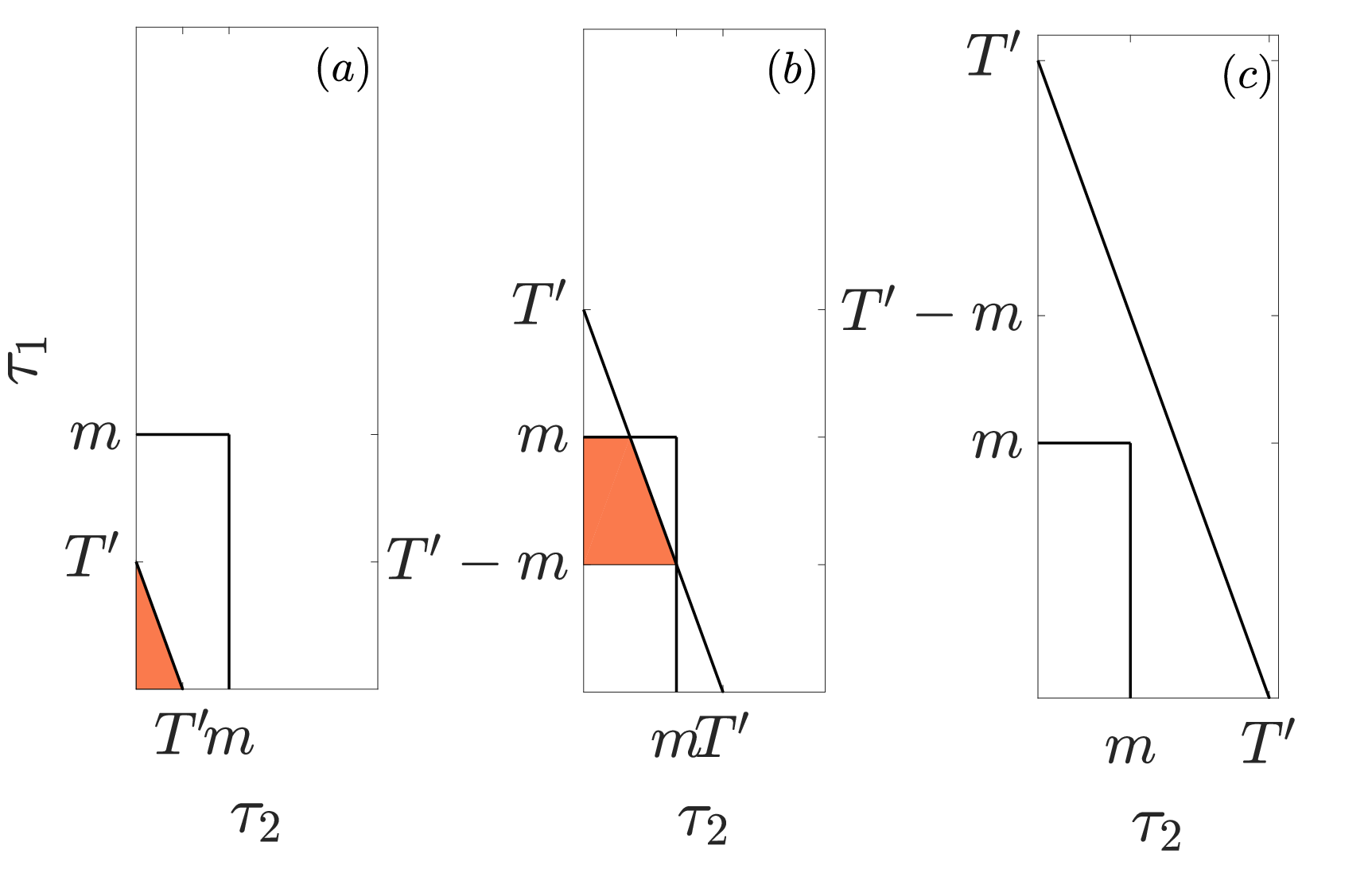
In order to finish the proof of Eq. (79) we show it for while assuming that the statement is true for . We write again the definition of the integral
| (86) |
We rearrange the order of integration and separate in the delta function
| (87) |
Now we consider which corresponds to regime (a) from Eq. (84). From this it is obviously because . This inequality is exactly the condition for which the -multiple integral inside the square bracket of Eq. (87) is the -fold convolution
| (88) |
according to the assumption of the induction proof. The remaining integral over is zero from to . The difference is positive because all are positive. So when we cannot fulfill the constrain. This property is controlled by the convolution in the integrand of Eq. (88) which is zero for negative arguments. So we get
| (89) |
and this is the convolution. Remember that we assumed in Eq. (88). Therefore we showed Eq. (79).
With the same arguments Eq. (79) can also be stated for discrete random variables with some arbitrary constraint . It is equivalently
| (90) |
for . For ZRP it is and and for TIDSI it is and . For ZRP and TIDSI the functions are for all .
Appendix B Typical fluctuations of TIDSI for the parameter
In bar2016exact the typical fluctuations of in the second half where calculated as
| (91) |
with the function
| (92) |
The hypergeometric function defined as
| (93) |
with the Pochhammer symbol .
We show now that Eq. (91) is identical to our result from Eq. (69). For that let us first take the derivative of the right hand side of Eq. (91) while :
| (94) |
where we used . Now we take out the term so that
| (95) |
To show the identity to Eq. (69) we have to show that the expression inside the big squared bracket of Eq. (95) is identical to . Let us write this question shortly as
| (96) |
i.e. is this statement true?
Here , and .
Since the hypergeometric function depends on we consider the series expansion at of the inner bracket. In principle any other point could be considered but the problem becomes simpler at . The Taylor series of Eq. (96) is
| (97) |
We apply the general Leibniz rule of derivation
| (98) |
The derivatives of and are
| (99) |
The two sums in Eq. (98) are only nonzero for and . Thus we can write
| (100) |
The binomial is zero when and so this expression is valid for all . Now we express the hypergeometric function by via the relationship of their derivatives. The -th derivative of the hypergeometric function at is
| (101) |
thus
| (102) |
So we can write
| (103) |
We order according to the hypergeometric functions
| (104) |
With Eq. (99) we get
| (105) |
Now we split the summation over for and all other . For the latter we use the relationship between successive orders of the derivative for the hypergeometric function
| (106) |
valid for . This gives zero for all terms with in Eq. (105) and only the term with remains. With we obtain
| (107) |
Thus we finally showed that indeed
| (108) |
References
- (1) J.-P. Bouchaud and M. Mézard, J. Phys. A Math. Gen. 30, 7997 (1997).
- (2) S. Albeverio, V. Jentsch, and H. Kantz, Extreme Events in Nature and Society (Springer Verlag, Berlin Heidelberg, 2006).
- (3) P. Embrechts, C. Klüppelberg, and T. Mikosch, Modelling Extremal Events: for Insurance and Finance, vol. 33 (Springer Verlag, Berlin Heidelberg, 2013).
- (4) J.-Y. Fortin and M. Clusel, J. Phys. A Math. Theor. 48, 183001 (2015).
- (5) S. N. Majumdar, A. Pal, and G. Schehr, Phys. Rep. 840, 1 (2020).
- (6) B. Meerson and S. Redner, Phys. Rev. Lett. 114, 198101 (2015).
- (7) Z. Schuss, K. Basnayake, and D. Holcman, Phys. Life Rev. 28, 52 (2019).
- (8) W. Wang, A. Vezzani, R. Burioni, and E. Barkai, Phys. Rev. Res. 1, 033172 (2019).
- (9) D. Hartich and A. Godec, J. Phys. A Math. Theor. 52, 244001 (2019).
- (10) L. Zarfaty, E. Barkai, and D. A. Kessler, arXiv:2006.13677 (2020).
- (11) E. J. Gumbel, Statistics of Extremes (Dover, New York, 1958).
- (12) R. A. Fisher and L. H. C. Tippett, 24, 180 (1928).
- (13) C. Godrèche and J. Luck, J. Stat. Phys. 104, 489 (2001).
- (14) M. Niemann, E. Barkai, and H. Kantz, Math. Model. Nat. Pheno. 11, 191 (2016).
- (15) W. Wang, J. H. Schulz, W. Deng, and E. Barkai, Phys. Rev. E 98, 042139 (2018).
- (16) W. Feller, An Introduction to Probability Theory and Its Applications, vol. 2 (Wiley, New York, 1971).
- (17) S. B. Lowen and M. C. Teich, Phys. Rev. E 47, 992 (1993).
- (18) M. Evans, S. N. Majumdar, and R. Zia, J. Stat. Phys. 123, 357 (2006).
- (19) S. Majumdar, Exact Methods in Low-dimensional Statistical Physics and Quantum Computing: Lecture Notes of the Les Houches Summer School: Volume 89, July 2008 407 (2010).
- (20) S. N. Majumdar, M. Evans, and R. Zia, Phys. Rev. Lett. 94, 180601 (2005).
- (21) R. Zia, M. Evans, and S. N. Majumdar, J. Stat. Mech. Theory Exp. 2004, L10001 (2004).
- (22) M. R. Evans and T. Hanney, J. Phys. A Math. Gen. 38, R195 (2005).
- (23) A. Bar and D. Mukamel, Phys. Rev. Lett. 112, 015701 (2014).
- (24) A. Bar and D. Mukamel, J. Stat. Mech. Theory Exp. 2014, P11001 (2014).
- (25) C. Godrèche, S. N. Majumdar, and G. Schehr, Phys. Rev. Lett. 102, 240602 (2009).
- (26) C. Godrèche, S. N. Majumdar, and G. Schehr, J. Phys. A-Math Theor. 47, 255001 (2014).
- (27) C. Godrèche, S. N. Majumdar, and G. Schehr, J. Stat. Mech. Theory Exp. 2015, P03014 (2015).
- (28) A. Vezzani, E. Barkai, and R. Burioni, Phys. Rev. E 100, 012108 (2019).
- (29) C. L. Scheffer, Stoch. Process. Their Appl. 55, 101 (1995).
- (30) M. R. Evans and S. N. Majumdar, J. Stat. Mech. Theory Exp. 2008, P05004 (2008).
- (31) A. Bar, S. N. Majumdar, G. Schehr, and D. Mukamel, Phys. Rev. E 93, 052130 (2016).
- (32) C. Godrèche, J. Phys. A Math. Theor. 50, 195003 (2017).
- (33) J. Wendel, Math. Scand. 14, 21 (1964).
- (34) A. Rebenshtok, S. Denisov, P. Hänggi, and E. Barkai, Phys. Rev. Lett. 112, 110601 (2014).
- (35) T. Akimoto, E. Barkai, and G. Radons, Phys. Rev. E 101, 052112 (2020).
- (36) D. A. Kessler and E. Barkai, Phys. Rev. Lett. 105, 120602 (2010).
- (37) X. Wang, W. Deng, and Y. Chen, J. Chem. Phys. 150, 164121 (2019).
- (38) T. Akimoto, S. Shinkai, and Y. Aizawa, J. Stat. Phys. 158, 476 (2015).
- (39) T. Akimoto and T. Miyaguchi, Phys. Rev. E 82, 030102 (2010).
- (40) F. D. Stefani, J. P. Hoogenboom, and E. Barkai, Phys. Today 62, 34 (2009).
- (41) G. Margolin and E. Barkai, Phys. Rev. Lett. 94, 080601 (2005).
- (42) R. Metzler and J. Klafter, Phys. Rep. 339, 1 (2000).
- (43) R. Kutner and J. Masoliver, Eur. Phys. J. B 90, 50 (2017).
- (44) D. R. Cox, Renewal theory (Methuen Publishing Ltd, London, 1962).
- (45) J. Lamperti, Am. Math. Soc 12, 724 (1961).
- (46) A. Vezzani, E. Barkai, and R. Burioni, Sci. Rep. 10, 1 (2020).
- (47) R. Burioni and A. Vezzani, J. Stat. Mech. Theory Exp. 2020, 034005 (2020).
- (48) H. Touchette, Phys. Rep. 478, 1 (2009).
- (49) W. Wang, M. Höll, and E. Barkai, arXiv:1908.03580 (2020).
- (50) C. Godrèche, arXiv:2006.04076 (2020).