Deep-Learning Study of the 21cm Differential Brightness Temperature During the Epoch of Reionization

We use the 21cmFASTMesinger et al. 2011 to generate the 21-cm signal and corresponding neutral fraction with the redshifts $z=6\sim 13$, where most of the current studies strongly have constrained. The 21cmFAST is the publicly-available simulation of the cosmological reionization which is self-consistent and semi-numerical. Specifically, this is optimized to generate the 21-cm signal during the epoch. By the combinations of the excursion-set formalismBond et al. 1991; Furlanetto et al. 2004 which mentioned earlier for identifying ionized hydrogen regions and the first-order perturbation theoryZel’Dovich 1970, it generates the full three-dimensional realizations of the density, ionization field, velocity, and spin temperature and finally the 21-cm differential brightness temperature with a given redshift.

We first generate the density and velocity fields with $50$, $100$, $200$, and $300\mathinner{\mathrm{Mpc}}$ comoving boxsizes and $800^{3}$, $1000^{3}$, and $1250^{3}$ grids between $z=6\sim 13$. We use different random seeds to generate the initial conditions for each combination of comoving boxsize and grid number, and, as a result, we get 12 independent simulation sets. For each simulation set, we obtain $18\sim 35$ snapshots between $z=6\sim 13$, where the number of snapshots depends on the number of grids. Note that the spatial resolutions used in this paper ($\Delta x=0.04\sim 0.375\mathinner{\mathrm{Mpc}}$) are smaller than the length scale where density perturbation from the 21cmFAST agrees well with the $N$-body simulationsMesinger et al. 2011. However, since we do not focus on small-scale details and the output 21-cm maps would be smoothed in larger scales, our choice of spatial resolution does not severely affect our result.

Then we calculate the “undistorted” 21-cm differential brightness temperature, $\delta T_{\rm b}^{0}(\bm{\mathbf{x}},z)$, by downgrading the resolution to $200^{3}$ grids:

where $\delta$, $T_{\rm CMB}$, and $T_{\rm S}$ are the gas overdensity, the CMB temperature, and the gas spin temperature, respectivelyMorales and Wyithe 2010. In 21cmFAST, $T_{\rm S}(z)$ is calculated from the evolution of the kinetic gas temperature and the Ly-$\alpha$ background. Also, $x_{\rm HI}(\bm{\mathbf{x}},z)$ is calculated from the number of IGM ionizing photons per baryon Park et al. 2019

where $\bar{\rho_{\rm b}}$, $M_{\rm h}$, $f_{\rm duty}$, $M_{\star}$, $f_{\rm esc}$, $N_{\gamma/{\rm b}}$ are the mean baryon density, halo mass, factor related to the suppression of star formation at massive halos, stellar mass, escape fraction, and the number of ionizing photons per stellar baryon, respectively. $f_{\rm duty}$, $M_{\star}$, and $f_{\rm esc}$ can be expressed as a function of $M_{\rm h}$ as follows:

where $M_{\rm turn}$ is the halo mass threshold for efficient star formation, and $f_{\star}$ is the fraction of galactic gas in stars. In this paper, we adopt a fiducial setup in Park et al. 2019 for reionization parameters: $(N_{\gamma/{\rm b}},f_{\star,10},\alpha_{\star},f_{\rm esc,10},\alpha_{\rm esc},M_{\rm turn})=(5000,0.05,0.5,0.1,-0.5,5\times 10^{8}\mathinner{\mathrm{M}_{\odot}})$. Note that we do not test different values of reionization parameters in this paper, mainly because we focus on the evolution of the mean neutral hydrogen fraction $\bar{x}_{\rm HI}(z)$ rather than constraining the reionization model.

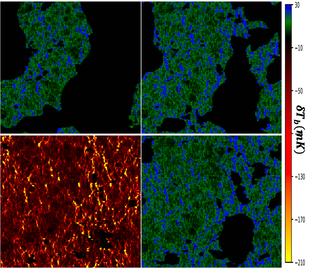
Figure 1 shows an example of undistorted 21-cm maps in a $50\,{\rm cMpc}$-box. As expected in Eq. (1) (if $T_{\rm S}\gg T_{\rm CMB}$, which is believed to be satisfied during the main reionization epoch), the undistorted 21-cm maps are proportional to the matter density and follow Gaussian distribution at high $(z,\bar{x}_{\rm HI})$. On the other hand, at low $(z,\bar{x}_{\rm HI})$, the overdense region becomes fully ionized and shows no 21-cm signal, and therefore, the distribution is highly non-Gaussian. Note that the estimation of $\bar{x}_{\rm HI}$ from the undistorted 21-cm maps could be rather straightforward, as it is simply the fraction of area where $x_{\rm HI}(\bm{\mathbf{x}})$ is close to zero. However, the estimation of $\bar{x}_{\rm HI}$ may not be that straightforward if one adds the observational effects to the 21-cm signal, which we will see in the next section.

In practice, we expect that the observed signal would be very different with Figure 1, because the actual observational signal will be obtained by integrating the angle, frequency, and observation time. At this point, the size of the angle and frequency are the limit of spatial and depth resolution of the telescope. As the size of the angle or frequency of the telescope becomes larger, the observed signal becomes more smoothed. Then the small-scale information is lost and the estimation of $\bar{x}_{\rm HI}$ similar to that we mentioned at the previous section may fail. On the other hand, the smaller angle or frequency could contain the small-scale information. However, if the integration time is fixed, the level of noise becomes higher and the estimation of $\bar{x}_{\rm HI}$ could be also difficult. Therefore, it is essential to include such observational effects, i.e., smoothing and noise, for the performance test of analysis methods such as our CNN model.

We start from smoothing the undistorted 21-cm maps with given angle and frequency setup of radio telescope. Here, we use three choices of the beamsizes and frequency bandwidths—$\Delta\theta=1^{\prime}$, $2^{\prime}$, and $3^{\prime}$, and $\Delta\nu=0.2\mathinner{\mathrm{MHz}}$, $1\mathinner{\mathrm{MHz}}$, and $2\mathinner{\mathrm{MHz}}$. The corresponding comoving length scales for given $\Delta\theta$ and $\Delta\nu$ are

where $D_{c}(z)$ is the comoving distance, and $\nu_{0}=1420\mathinner{\mathrm{MHz}}$ is the rest-frame frequency of the 21-cm line. Note that the subscripts ‘$\perp$’ and ‘$\parallel$’ emphasize that the beamsize and frequency bandwidth affect the smoothing of $\delta T_{\rm b}$ in directions perpendicular and parallel to the line-of-sight (LOS), respectively.

The actual shape of smoothing kernels in directions parallel and perpendicular to the LOS ($W(\nu;\Delta\nu)$ and $W(\theta;\Delta\theta)$, respectively) strongly depends on the configuration of radio telescope, even with the identical choice of $(\Delta\theta,\Delta\nu)$. Especially, the shape of $W(\theta;\Delta\theta)$ (beam shape) could greatly vary depending on the antennae design. It is known that some “dirty” beam shape such as the compensated Gaussian kernel might be possibleMellema et al. 2006, and in that case the understanding of the $\bar{x}_{\rm HI}(z)$ could be extremely difficultHong et al. 2014. Nevertheless, for simplicity and because the configuration of future surveys is not fixed, we assume the Gaussian kernel for both beam and frequency smoothing kernels in this paper. We use $\Delta\theta$ and $\Delta\nu$, or identically, $\Delta L_{\perp}$ and $\Delta L_{\parallel}$, as the full-width half-maximum of the beam and frequency smoothing kernel.

Also, since interferometric radio observations might be insensitive to the large-scale fluctuation of $\delta T_{\rm b}$, we subtract the mean of the smoothed 21-cm signal from the map so that the average of the subtracted 21-cm map becomes zero. In summary, we obtain the “smoothed” 21-cm map (or, $\delta T_{\rm b}^{\rm s}(\bm{\mathbf{\theta}},\nu)$, where $\nu=\nu_{0}/(1+z)$) as follows:

Here, the subscript ‘G’ emphasizes the Gaussian kernel.

Figure 2 shows an example of the smoothed mock 21-cm map in a $300\,{\rm cMpc}$-box at $(z,\bar{x}_{\rm HI})=(12.73,0.97)$. Compared to the undistorted 21-cm maps in Figure 1, there exists two key features in smoothed maps that make the estimation of $\bar{x}_{\rm HI}(z)$ more difficult. First of all, due to the mean subtraction after smoothing, we cannot use the mean value ($\langle\delta T_{\rm b}^{\rm s}(\bm{\mathbf{\theta}},\nu)\rangle_{\bm{\mathbf{\theta}}}$) as an indicator of $\bar{x}_{\rm HI}(z)$, especially for high-$z$ cases (see the bottom-left panel of Figure 1 as a comparison). Additionally, smoothing in both parallel and perpendicular directions to the LOS wipes out the small-scale features. As a result, without a prior knowledge, the heavily smoothed 21-cm map at the lower-right panel of Figure 2 might be confused to be at the middle of EoR (e.g., $\bar{x}_{\rm HI}(z)\sim 0.5$). Note that, however, the spatial distribution of the smoothed 21-cm maps is Gaussian and highly non-Gaussian at $\bar{x}_{\rm HI}\simeq 1$ and $1-\bar{x}_{\rm HI}\gg 0$, respectively. Therefore, it may be possible to distinguish between the smoothed 21-cm maps before and the middle of EoR by using $n$-point correlation functions or Minkowski functionalsHong et al. 2014; Wang et al. 2015, while such methods usually require precise measurement of $\delta T_{\rm b}$.

After smoothing, we add the noise to the mock 21-cm maps, whose level depends on the integration time and the configuration of radio telescope. Here, we adopt the sensitivity limit at Hong et al. 2014, which uses the sensitivity calculation from Iliev et al. 2003 by assuming the SKA with core size of $\sim 1\,{\rm km}$. While the spatial and intensity distribution of noise and how it convolves with the signal also strongly depends on the configuration of radio telescopeAsorey et al. 2020, here we adopt a somewhat simple model as follows. We calculate the root-mean-square (RMS) of noise level ($\sigma(\Delta T;\Delta\theta,\Delta\nu)$) by using 10-, 100-, 1000-, and 10000-hour integration times and produce the Gaussian white noise with given RMS level and random seeds ($\epsilon$). Then we obtain the “noisy” 21-cm map (or, $\delta T_{\rm b}^{\rm n}(\bm{\mathbf{\theta}},\nu)$) by adding the noise to the smoothed 21-cm map,

Note that the mean value of the noisy 21-cm map remains zero.

Figure 3 shows the comparison between our sensitivity limit estimation and the RMS value of the smoothed mock 21-cm maps ($\delta T_{\rm b,rms}$) with various configurations of beamsize, frequency bandwidth, and integration time. Here, $\delta T_{\rm b,rms}/\sigma$ can be regarded as a proxy of the signal-to-noise ratio (SNR). As commented earlier, to fully utilize the advantages of some $n$-points or topological analysis methods, one needs to achieve ${\rm SNR}\gg 1$. By assuming marginal choices of beamsize and frequency bandwidth, e.g., $\Delta\theta=1^{\prime}\sim 2^{\prime}$ and $\Delta\nu=1\sim 2\mathinner{\mathrm{MHz}}$, such SNR is possible only with $\gtrsim 10000$-hour SKA integration timeHong et al. 2014.

Figure 4 further shows how adding noise affects the same mock 21-cm maps to Figure 2, by assuming 1000-hour SKA integration time. At large beamsize and frequency bandwidth (e.g., bottom-right panel of Figure 4), the RMS value of the smoothed mock 21-cm maps is higher than the sensitivity limit. Also, the overall distribution of the noisy 21-cm map is similar to the smoothed 21-cm map. On the other hand, at small beamsize and frequency bandwidth (e.g., top-left panel of Figure 4), the RMS value is about an order of magnitude smaller than the sensitivity limit. As a result, sophisticated analysis methods that rely the detailed spatial distribution of $\delta T_{\rm b}^{\rm n}$ might find difficulties in such maps without an additional denoising process.

Note that, however, one can see a visual pattern of patches with generally positive and negative values of $\delta T_{\rm b}^{\rm n}$ at the top-left panel of Figure 4, even before any denoising process. Also, one can see that such visual pattern has similarity to the clearer patterns shown at other panels (i.e., noisy 21-cm maps with larger beamsize and frequency bandwidth). However, although there exist some candidates such as binning or Gaussian smoothing, the mathematical definition of such “visual pattern” may not be straightforward. Note that such recognition of mathematically unclear visual patterns is one of the strongest specialties of deep learning technique, which we will see in the next section.

We use the convolutional neural network (CNN) optimized to recognize visual patterns within the image dataset with efficiently lessening computational cost for expressing complex non-linear function for multi-dimensional input data. Figure 5 and Table 1 show our CNN architecture design. The entire network is divided into two parts, feature extraction and (fully-connected; FC) linear regression. All the filters in the first part of the architecture have the same size, $(3,3)$, and are employed to extract the feature of the processed 21-cm map through a series of convolutions. Before each convolution layer, we use the max pooling (MaxPool) layer. The MaxPool layer helps to ease operations needed over the training by reducing the features resulting from convolution one, and can improve the result by keeping the network from getting over-fitted with a represented value (c.f. maximum or mean) of particular features over from the local regions, without numerous feature maps more than necessary. Finally, after the convolution and pooling layers, it is followed by a linear regression part, which consists of three FC layers. The FC layers employ the high-level features from the first part of the CNN and help to learn the network be close to have a desired output value through the last fully-connected layer activated by a linear function.

We apply the rectified linear unit (ReLU), which is defined as ${\rm ReLU}(s)=\max(0,s)$, as the activation functions of all convolutional and FC layersHahnloser et al. 2000; Glorot et al. 2011. The weights on the fully-connected layers are initialized by applying He uniform initializationHe et al. 2015, which extract $n_{\rm in}$ samples from weights initialized from a uniform distribution between $-\sqrt{6/n_{\rm in}}$ and $+\sqrt{6/n_{\rm in}}$. The He uniform initialization for weights technique helps in reaching a global minimum of the cost function faster and more effectively.

Before each ReLU activation, we also add batch normalization (BatchNorm) layersIoffe and Szegedy 2015. For the situation where the inputs are fed with forwarding to the output layer, the distributions of inputs keep changing with each iterations because the weights of each layers are changed over the training of network. So the intermediate layers are hard to adapt its changing distributions of inputs. To prevent such problems, BatchNorm renormalize a mini-batch of inputs ($x_{i}$) into $y_{i}$ as:

where $\mu$ and $\sigma$ are the mean and standard deviation of $x_{i}$, $\epsilon$ is a small constant value introduced to avoid divergence, and $\gamma$ and $\beta$ are two additional learnable parameters introduced in the BatchNorm process. Not only BatchNorm can effectively complement some chronic problems that deep neural network has, such as gradient vanishing problem, but allow us to use much higher learning rate and perform as a regularizer for a part.

For the CNN training, first of all, we produce the samples by splitting the noisy 21-cm maps with $200^{3}$ grids into 67 slices of $200\times 200$ pixels along the LOS direction. We calculate the mean neutral hydrogen fraction for each slice. Note that, while we only use $18\sim 35$ snapshots between $z=6\sim 13$, $\bar{x}_{\rm HI}$ estimated from different slices at the same redshift may vary. As a result, for a given $(\Delta\theta,\Delta\nu,\Delta T)$, we have $1206\sim 2345$ samples for each boxsize and high-resolution grid setup. Note that the difference of angular field of view from a fixed boxsize between $z=6\sim 13$ is less than $13\%$, which we will consider as nearly identical. We have also found that the performance is similar even if one uses 10318 samples from all 9 boxsize- and high-resolution-grid-setups, and therefore, we use all 10318 samples hereafter.

We produce the inputs of our CNN architecture by converting each $200\times 200$ pixels of $\delta T_{\rm b}^{\rm n}$ slice into a 3-channel RGB image (i.e., an array with $(3,200,200)$ size) by applying a custom colormap scheme (see Table 2 for definition and Figure 6 for examples). We have also tested using the $200\times 200$ slice directly as input and found no notable difference in performance.

We then split our samples into three sets: training set used for training the model parameters, validation set used for checking the training process, and test set for evaluating the performance of the trained model. For a given $(\Delta\theta,\Delta\nu,\Delta T)$, we split 10318 samples to 7428 training samples, 826 validation samples, and 2064 test samples. We randomly split the samples into three sets while keeping the distribution of $\bar{x}_{\rm HI}$ similar.

We compile our CNN model with Adam optimizerKingma and Ba 2014 with a learning rate $10^{-3}$. Also, we adopt the mean squared error (MSE) as the loss function,

Here, $m$ is the minibatch size for training, which is set to 8. We have also tested several minibatch sizes between 4 and 64 and found no notable difference in performance for $m\geq 8$.

We define an epoch as an iteration of fitting the model parameters from 7428 training samples and evaluating its training loss as well as validation loss from 826 validation samples. Since we set the minibatch size to 8, the number of minibatches per epoch is 929. For a single run of CNN training, we set the maximum number of epochs as 500. However, for saving the time and preventing the overfitting, we stop the training when the validation loss is not improved for 30 epochs, and the typical number of epochs becomes $\sim 200$. We then use the model at the epoch where the validation loss is minimized. We perform our training with KerasChollet et al. 2015 with Tensorflow GPU version as a backendAbadi et al. 2015, and each run takes $\sim 2$ hours with a single NVIDIA V100 GPU card in a NVIDIA DGX-1 GPU platform.

Furthermore, we make use of the cross validation (CV) technique to test the stability of a certain deep learning model. In CV technique, the entire dataset is split into $K$-folds, and multiple CNN models are trained by using a certain fold as validation set and the remaining $(K-1)$-folds as training set. We use the shuffled 10-folded CV so that we train our network 5 times with the number of epoch and data having different distribution for each time. We have found that the validation loss from different models agrees within less than $75\%$ deviation from their average.