A curious correspondence has been known between Landau models and non-linear sigma models: Reinterpreting the base-manifolds of Landau models as field-manifolds, the Landau models are transformed to non-linear sigma models with same global and local symmetries. With the idea of the dimensional hierarchy of higher dimensional Landau models, we exploit this correspondence to present a systematic procedure for construction of non-linear sigma models in higher dimensions. We explicitly derive $O(2k+1)$ non-linear sigma models in $2k$ dimension based on the parent tensor gauge theories that originate from non-Abelian monopoles. The obtained non-linear sigma models turn out to be Skyrme-type non-linear sigma models with $O(2k)$ local symmetry. Through a dimensional reduction of Chern-Simons tensor field theories, we also derive Skyrme-type $O(2k)$ non-linear sigma models in $2k-1$ dimension, which realize the original and other Skyrme models as their special cases. As a unified description, we explore Skyrme-type $O(d+1)$ non-linear sigma models and clarify their basic properties, such as stability of soliton configurations, scale invariant solutions, and field configurations with higher winding number.

1 Introduction

Non-linear sigma (NLS) models were originally introduced for a description of mesons in hadron physics around 1960 [1, 2, 3, 4, 5, 6]. Skyrme proposed his celebrated NLS model with a higher derivative term [7] to describe baryons as solitonic excitations of meson fluid. We refer to such non-linear sigma models with a higher derivative term as the Skyrme-type non-linear sigma model (S-NLS) in this paper. The Skyrmions, or more generally the NLS model topological solitons, accommodate deep mathematical structure related to gauge theories. In particular, relationship between the quaternionic projective non-linear sigma model and $SU(2)$ gauge theory was intensively investigated around 1970 [8, 9, 10, 11, 12, 13, 14, 15, 16, 17]. The self-dual equations of higher dimensional gauge theories were also revealed in 1980s [18, 19, 20, 21, 22, 23, 24, 25, 26]. An explicit recipe for derivation of the Skyrmion field configuration from the $SU(2)$ instanton was proposed by Atiyah and Manton [27, 28], which stimulated recent studies about connections of topological solitons in different dimensions, [29, 30, 31, 32, 33, 34] and [35, 36, 37, 38, 39, 40, 41]. Apart from such formal aspects, Skyrmions now appear ubiquitously in many branches of theoretical physics [42] and are also observed in daily nanoscale magnetic experiments (see [43] and references therein).

One of the most prominent early experiments about Skyrmions, more precisely $O(3)$ NLS model solitons, is the NMR Knight shift measurement of the spin texture in quantum Hall ferromagnets [44]. Besides of the quantum Hall ferromagnets, we often come across the $O(3)$ NLS model solitons in various contexts of the quantum Hall effect. One example is about anyonic excitations of the fractional quantum Hall effect. The effective field theory of the fractional quantum Hall effect is the Chern-Simons topological field theory [45, 46, 47]. The Chern-Simons statistical field coupled to the $O(3)$ NLS model solitons provides a field theoretical description of anyons [48, 49] and such anyons are realized as fractionally charge excitations of the fractional quantum Hall effect [50, 51]. Another important example is about their analogous mathematical structures. The Haldane’s formulation of the quantum Hall effect [52] is based on the $SO(3)$ Landau model [53, 54] in the Dirac monopole background [55], in which the $\it{base\text{-}manifold}$ or physical space is given by $S^{2}$ and the gauge symmetry is $U(1)$ . Meanwhile in the $O(3)$ NLS model [56, 57] or equivalently the $\mathbb{C}P^{1}$ model [58, 59, 60], the $\it{target\text{-}manifold}$ manifold or the field-space is $S^{2}\simeq\mathbb{C}P^{1}$ and the hidden local symmetry is $U(1)$ .¹¹ 1 We used $``SO(3)^{\prime\prime}$ for the Landau model, since the Landau model Hamiltonian is constructed by the angular momentum operators of the $SO(3)$ group, while $``O(3)^{\prime\prime}$ for the NLS model since the NLS model Hamiltonian is invariant under the $O(3)$ transformation, $i.e.$ , $SO(3)$ rotations and $\mathbb{Z}_{2}$ reflection of the NLS field. One may find a curious correspondence between the Landau model and the NLS model: The base-manifold $S^{2}$ of the Landau model is identical to the target-manifold of the $O(3)$ NLS model, and their local symmetries are also given by $U(1)$ . We will refer to this correspondence as the Landau/NLS model correspondence.

The Landau/NLS model correspondence is not a special property in 2D, but holds in 4D. In the 4D quantum Hall effect [61], the Landau model is given by the $SO(5)$ Landau model [62, 63] whose base-manifold is $S^{4}$ and magnetic field background is given by the Yang’s $SU(2)$ monopole [64]. Meanwhile in the $O(5)$ NLS model or the $\mathbb{H}P^{1}$ model [8, 9, 13, 14, 15, 16, 17], the field-manifold is $S^{4}$ and the hidden local symmetry is $SU(2)$ . Besides, anyonic excitations in the 4D quantum Hall effect are known to be membrane-like objects whose internal space is $S^{4}$ described by the field-manifold of the $O(5)$ NLS model [65, 66]. The Landau/NLS model correspondence is thus reasonably generalized from 2D to 4D. It may be natural to ask whether the Landau/NLS model correspondence can hold in even higher dimensions. Such correspondence indeed holds in arbitrary dimensions as suggested in [67]. Quantum Hall effect on arbitrary $d$ -dimensional sphere has been constructed in [67, 68, 69]²² 2 See [70, 71] and references therein about early developments of the higher dimensional quantum Hall effect. (see [72, 73] also), and the mathematical set-up is given by the $SO(d+1)$ Landau model in the $SO(d)$ monopole background. The excitations are $(d-2)$ -dimensionally extended anyonic objects whose fractional statistics are well investigated in [74, 75, 76, 77, 78]. The effective field theory is a tensor-type topological field theory coupled to the $(d-2)$ -brane with $S^{d}$ internal space, which is described by the field-manifold of $O(d+1)$ NLS models [67, 69]. Again, the field-manifold of the NLS model is identical to the base-manifold of the quantum Hall effect. Furthermore, it is widely known that any $O(d+1)$ NLS models with field-manifold $S^{d}\simeq O(d+1)/O(d)$ possess the hidden local symmetry $O(d)$ [79, 80, 81]. The Landau/NLS model correspondence thus actually holds in arbitrary dimensions.

While NLS model solitons play crucial roles in the higher dimensional quantum Hall effect, a systematic analysis of the $O(d+1)$ NLS model to host membrane excitations is still lacking. To be more precise, there are numerous possible NLS models with field-manifold being $S^{d}$ , but there is no criterion to choose better models or hopefully the best model among these models. A main purpose of this paper is to provide a systematic procedure to construct appropriate NLS models based on the Landau/NLS model correspondence [Fig.1]. For the construction, we make use of the idea of the dimensional hierarchy of the higher dimensional Landau models [67, 68, 69]. Consequently, the obtained NLS models necessarily inherit structures of the differential geometry of the Landau models.

Refer to caption — Figure 1: The Landau/NLS model correspondence for $d=2k$ . The differential topological structure of the $SO(2k+1)$ Landau model is same as of the $O(2k+1)$ NLS model. The Landau model is transformed to the NLS model under identification of the base-manifold with the field-manifold.

We also adopt the idea that was originally suggested by Tchrakian [18] and recently made manifest by Adam et al. [82] where a BPS equation is firstly given and the Hamiltonian is later derived so that the Hamiltonian may satisfy the BPS equation.

The paper is organized as follows. Sec.2 reviews the differential geometry associated with non-Abelian monopoles in the higher dimensional Landau models. In Sec.3, we reconsider geometric meanings of the Skyrme’s NLS field and the $O(5)$ S-NLS model in the light of the Landau/NLS model correspondence. We present a systematic method for derivation of $O(2k+1)$ S-NLS models and explicitly construct the $O(7)$ NLS model and $O(2k+1)$ NLS model Hamiltonians in Sec.4. In Sec.5, we construct $O(2k)$ S-NLS models using the Chern-Simons term of pure gauge fields. We explore general $O(d+1)$ S-NLS models and analyze their basic properties in Sec.6. Sec.7 is devoted to summary and discussions.

2 Differential Geometry of the Higher Dimensional Landau Model

In this section, we review the differential geometry of the $SO(2k+1)$ Landau models and discuss extended objects that are realized as the $O(2k+1)$ NLS model solitons.

2.1 Non-Abelian monopole configuration of the $SO(2k+1)$ Landau model

The $SO(5)$ Landau model is formulated on $S^{4}$ embedded in $\mathbb{R}^{5}$ [61, 62, 63], and the background magnetic field is given by the Yang’s $SU(2)$ monopole [64]

A=-\frac{1}{2r(r+r_{5})}\eta_{mn}^{i}r_{n}\sigma_{i}dr_{m},~~~~(m,n=1,2,3,4)

(1)

where $\eta_{mn}^{i}\equiv\epsilon_{mni4}+\delta_{mi}\delta_{n4}-\delta_{m4}\delta_{ni}$ denotes the ’t Hooft symbol [83]. The 1D reduction of the $SO(5)$ Landau model reproduces the $SO(4)$ Landau model [84, 85] on the $S^{3}$ -equator of $S^{4}$ [63, 86]. In Sec.3, we will consider the reverse process to derive the $O(5)$ S-NLS model from the Skyrme’s field-manifold $S^{3}$ .

Generalizing the $SU(2)~(\otimes SU(2)\simeq SO(4))$ to the $SO(2k)$ group [87],³³ 3 To be precise, $Spin(2k)$ group. the $SO(2k+1)$ Landau model is introduced on a base-manifold $S^{2k}$ in the $SO(2k)$ monopole background [68, 67] [Table 1].

Landau model	$SO(3)$	$SO(5)$	$SO(2k+1)$
Base-manifold	${S}^{2}$	${S}^{4}$	$S^{2k}$
Global symmetry	$SO(3)\simeq SU(2)$	$SO(5)$	$SO(2k+1)$
Monopole gauge group	$SO(2)\simeq U(1)$	$SO(4)\simeq SU(2)~(\otimes SU(2))$	$SO(2k)$
Chern number	1st	2nd	$k$ th
Topological map	$\pi_{1}(U(1))\simeq\mathbb{Z}$	$\pi_{3}(SU(2))\simeq\mathbb{Z}$	$\pi_{2k-1}(SO(2k))\simeq\mathbb{Z}$

Table 1: Geometric and topological features of the Landau models. The monopole gauge group

SO(2k)

is chosen so that it is identical to the holonomy group of the base-manifold

S^{2k}\simeq SO(2k+1)/SO(2k)

[68]. In the

SO(5)

Landau model, the holonomy of

S^{4}

SO(4)\simeq SU(2)\otimes SU(2)

and one of the two

SU(2)

s is adopted as the gauge group.

Notice that the gauge group is equal to the holonomy group of the basemanifold. The $SO(2k)$ monopole gauge field is represented as

A=\sum_{a=1}^{2k+1}A_{a}dr_{a}=-\frac{1}{r(r+r_{2k+1})}\sum_{m,n=1}^{2k}\sigma_{mn}r_{n}dr_{m},

(2)

A_{m}=-\frac{1}{r(r+r_{2k+1})}\sigma_{mn}r_{n},~~A_{2k+1}=0,~~~(m,n=1,2,\cdots,2k)

(3)

which is regular except for the south pole.⁴⁴ 4 At $r_{2k+1}=0$ , the $SO(2k)$ monopole configuration, (3) or (9), is reduced to the meron configuration on $\mathbb{R}^{2k}$ [88]: $A_{\mu}=-\frac{1}{x^{2}}\sigma_{\mu\nu}x_{\nu},~~~F_{\mu\nu}=\frac{1}{x^{2}}\sigma_{\mu\nu}-\frac{1}{x^{2}}(x_{\mu}A_{\nu}-x_{\nu}A_{\mu}),$ (4) which satisfies the pure Yang-Mills field equation on $\mathbb{R}^{2k}$ [89, 90]: $\frac{\partial}{\partial x_{\mu}}F_{\mu\nu}+i[A_{\mu},F_{\mu\nu}]=0.$ (5) Here, $\sigma_{mn}$ are $Spin(2k)$ matrix generators:

\sigma_{ij}=-i\frac{1}{4}[\gamma_{i},\gamma_{j}],~~~\sigma_{i,2k}=-\sigma_{2k,i}=\frac{1}{2}\gamma_{i}

(6)

that satisfy

[\sigma_{mn},\sigma_{pq}]=i(\delta_{mp}\sigma_{nq}-\delta_{mq}\sigma_{np}+\delta_{nq}\sigma_{mp}-\delta_{np}\sigma_{mq}).

(7)

$\gamma_{i}$ $(i=1,2,\cdots,2k-1)$ stand for the $SO(2k-1)$ gamma matrices. The $SO(2k)$ monopole field strength is derived as

F=dA+i{A}^{2}=\frac{1}{2}F_{ab}~dr_{a}\wedge dr_{b},

(8)

where $F_{ab}=\partial_{a}A_{b}-\partial_{b}A_{a}+i[A_{a},A_{b}]$ are

F_{mn}=\frac{1}{r^{2}}\sigma_{mn}-\frac{1}{r^{2}}(r_{m}A_{n}-r_{n}A_{m}),~~~F_{m,{2k+1}}=-F_{2k+1,m}=\frac{1}{r^{2}}(r+r_{2k+1})A_{m}.

(9)

(3) and (9) satisfy the field equations of motion of the pure Yang-Mills theory in $(2k+1)$ D:⁵⁵ 5 We will give an alternative verification of (10) in Appendix A.3.

D_{a}F_{ab}=\partial_{a}F_{ab}+i[A_{a},F_{ab}]=0.

(10)

One may need only the algebraic property of the $SO(2k)$ generators (7) to verify (10), and so the monopole gauge field (3) of any $Spin(2k)$ representation realizes a solution of the pure Yang-Mills field equation. The monopole configuration carries unit Chern number. Indeed, substituting (9) into the $k$ th Chern number

c_{k}=\frac{1}{k!(2\pi)^{k}}\int\text{tr}(F^{k}),

(11)

we have

N_{2k}=\frac{1}{{A}(S^{2k}_{\text{phys.}})}\int_{S^{2k}_{\text{phys.}}}\frac{1}{(2k)!}\epsilon_{a_{1}a_{2}\cdots a_{2k+1}}r_{2a+1}dr_{a_{1}}dr_{a_{2}}\cdots dr_{a_{2k}}=1,

(12)

with $A(S^{2k})$ being the area of $S^{2k}$ :

{A}(S^{2k})=\frac{2^{k+1}}{(2k-1)!!}\pi^{k}.

(13)

(12) implies that the Chern number for the monopole configuration is accounted for by the winding number (the Pontryagin index) from $S^{2k}_{\text{phys.}}$ to $S^{2k}_{\text{field}}$ :

\pi_{2k}(S^{2k})\simeq\mathbb{Z}.

(14)

Another expression of the $SO(2k)$ monopole gauge field is

A^{\prime}=-\frac{1}{r(r-r_{2k+1})}\bar{\sigma}_{mn}r_{n}dr_{m},

(15)

which is regular except for the north-pole. The two expressions of the monopole gauge fields, (2) and (15), are related by a gauge transformation on the $S^{2k-1}$ -equator of $S^{2k}$ :

A^{\prime}=g^{\dagger}Ag-ig^{\dagger}dg,

(16)

where $g$ denotes a transition function of the form

\displaystyle g=\frac{1}{\sqrt{r^{2}-{r_{2k+1}}^{2}}}1_{2^{k-1}}+i\frac{1}{\sqrt{r^{2}-{r_{2k+1}}^{2}}}\sum_{i=1}^{2k-1}r_{i}\gamma_{i}=\cos\theta~1_{2^{k-1}}+i\sin\theta\sum_{i=1}^{2k-1}\hat{r}_{i}\gamma_{i}=e^{i\theta\sum_{i=1}^{2k-1}\hat{r}_{i}\gamma_{i}}.

(17)

Here,

\hat{r}_{i}\equiv\frac{1}{\sqrt{r^{2}-{r_{2k+1}}^{2}-{r_{2k}}^{2}}}r_{i}~~~(i=1,2,\cdots,2k-1),~~~~\tan\theta\equiv\frac{1}{r_{2k}}\sqrt{r^{2}-{r_{2k+1}}^{2}-{r_{2k}}^{2}}.

(18)

$g(x)$ can also be regarded as a non-linear realization of $Spin(2k)$ associated with the symmetry breaking $SO(2k)~\rightarrow~SO(2k-1)$ with the broken generators $\gamma_{i}=2\sigma_{i,2k}~\in~Spin(2k)$ . $A$ and $A^{\prime}$ are simply represented as

A=i\frac{1}{2r}(r-r_{2k+1})dgg^{\dagger},~~~~A^{\prime}=-i\frac{1}{2r}(r+r_{2k+1})g^{\dagger}dg,

(19)

where

-idgg^{\dagger}=\frac{2}{r^{2}-{r_{2k+1}}^{2}}{\sigma}_{mn}r_{n}dr_{m},~~~~-ig^{\dagger}dg=-\frac{2}{r^{2}-{r_{2k+1}}^{2}}\bar{\sigma}_{mn}r_{n}dr_{m}.

(20)

The $k$ th Chern number (11) can be expressed as [67]

c_{k}=\frac{(-i)^{k-1}}{(2k-1)!2^{k-1}{A}(S^{2k-1}_{\text{}})}\int_{S^{2k-1}_{\text{}}}\text{tr}(-ig^{\dagger}dg)^{2k-1}=(-i)^{k-1}\frac{1}{(2\pi)^{k}}\frac{(k-1)!}{(2k-1)!}\int_{S^{2k-1}_{\text{}}}\text{tr}(-ig^{\dagger}dg)^{2k-1}

(21)

where $A(S^{2k-1})$ signifies the area of $(2k-1)$ -sphere:

{A}(S^{2k-1})=\frac{2\pi^{k}}{(k-1)!}.

(22)

The associated topology is indicated by

\pi_{2k-1}(SO(2k))~\simeq~\mathbb{Z}.

(23)

Substituting (17) into (21), we have

N_{2k-1}=\frac{1}{{A}(S^{2k-1})}\int_{S^{2k-1}}\frac{1}{(2k-1)!}\epsilon_{a_{1}a_{2}\cdots a_{2k}}r_{a_{2k}}dr_{a_{1}}dr_{a_{2}}\cdots dr_{a_{2k-1}}=1,

(24)

which denotes unit winding number from $S_{\text{phys.}}^{2k-1}$ to $S_{\text{field}}^{2k-1}$ , and yields the same result as (12), as it should be. The equivalence between (12) and (24) holds for other higher dimensional representations of gauge group matrix generators [69]. We thus find that there are two equivalent but superficially different representations of the $k$ th Chern number for the monopole field configuration:

1.

Winding number associated with $\pi_{2k}(S^{2k})\simeq\mathbb{Z}$ .
2.

Winding number associated with $\pi_{2k-1}(S^{2k-1})\simeq\mathbb{Z}$ .

We will utilize the first observation in the construction of the $O(2k+1)$ S-NLS models, and the second one in the construction of the $O(2k)$ S-NLS models. This will also be important in the discussions of topological field configurations (Sec.6.2).

2.2 Tensor gauge fields and extended objects

The $k$ th Chern number (11) can be expressed as

c_{k}=\frac{1}{k!(2\pi)^{k}}\int G_{2k},

(25)

where $G_{2k}$ denotes a $2k$ rank tensor field strength

G_{2k}=\text{tr}(F^{k})=\frac{1}{(2k)!}G_{a_{1}a_{2}\cdots a_{2k}}dr_{a_{1}}dr_{a_{2}}\cdots dr_{a_{2k}}

(26)

G_{a_{1}a_{2}\cdots a_{2k}}=\frac{1}{2^{k}}~\text{tr}(F_{[a_{1}a_{2}}F_{a_{3}a_{4}}\cdots F_{a_{2k-1}a_{2k}]})=\frac{1}{2^{k}}~\text{tr}(F_{[a_{1}a_{2}\cdots a_{2l-1}a_{2l}}F_{a_{2l+1}a_{2l+2}\cdots a_{2k-1}a_{2k}]}).

(27)

Here, we introduced the antisymmetric tensor field strength [18]

F_{a_{1}a_{2}\cdots a_{2l}}\equiv\frac{1}{(2l)!}~F_{[\mu_{1}\mu_{2}}F_{a_{3}a_{4}}\cdots F_{a_{2l-1}a_{2l}]}.

(28)

There are $[k/2]$ independent ways for the decomposition (27) in correspondence with $l=1,2,\cdots,[k/2]$ . $[k/2]$ signifies the maximum integer that does not exceed $k/2$ . Apparently, there exists a local degree of freedom in the decomposition [91]:

F_{a_{1}a_{2}\cdots a_{2l}}\cdot F_{a_{21+1}a_{2l+2}\cdots a_{2k}}=\lambda(x)~F_{a_{1}a_{2}\cdots a_{2l}}\cdot\frac{1}{\lambda(x)}~F_{a_{21+1}a_{2l+2}\cdots a_{2k}}.

(29)

For the non-Abelian monopole gauge field (9), we can evaluate (27) as [67]

G_{2k}=\frac{1}{2^{k+1}r^{2k+1}}\epsilon_{a_{1}a_{2}\cdots a_{2k}a_{2k+1}}r_{a_{2k+1}}dr_{a_{1}}dr_{a_{2}}\cdots dr_{a_{2k}},

(30)

G_{a_{1}a_{2}\cdots a_{2k}}=\frac{(2k)!}{2^{k+1}r^{2k+1}}\epsilon_{a_{1}a_{2}\cdots a_{2k+1}}r_{a_{2k+1}},

(31)

which signifies the $2k$ -rank tensor monopole field strength in its own right [92, 93], and the $(2k-1)$ -rank tensor gauge field $(dC_{2k-1}=G_{2k})$ [94] is coupled to $(2k-2)$ -dimensionally extended objects, $i.e.$ , $(2k-2)$ -branes. In the higher dimensional quantum Hall effect, the size of the gauge space is comparable with the size of the base-manifold $S^{2k}$ [67], and the whole system is regarded as a $(4k-1)$ D space-time. The $(2k-2)$ -brane current in $(4k-1)$ D space-time is simply given by

J_{\mu_{1}\mu_{2}\cdots\mu_{2k-1}}=\frac{1}{(2k)!}\epsilon_{\mu_{1}\mu_{2}\cdots\mu_{4k-1}}\epsilon_{a_{1}a_{2}\cdots a_{2k+1}}n_{a_{1}}\partial_{\mu_{2k}}n_{a_{2}}\partial_{\mu_{2k+1}}n_{a_{3}}\cdots\partial_{\mu_{4k-1}}n_{a_{2k+1}},

(32)

where $n_{a}$ denote the internal field coordinates of the $(2k-2)$ -brane (the blue sphere of left of Fig.1). A simple subtraction, $(4k-1)-(2k-2)=2k+1$ , implies that the dimension of the internal space of the $(2k-2)$ -brane is $2k$ D and is naturally described by the $S^{2k}$ field-manifold of $O(2k+1)$ NLS models. Indeed, (32) is identical to the topological current of the $O(2k+1)$ NLS model soliton in $(4k-1)$ D space-time with coordinates $n_{a}$ subject to $\sum_{a=1}^{2k+1}n_{a}n_{a}=1$ . Notice that the obtained field-manifold is same as the original base-manifold $S^{2k}$ . Furthermore, the $(2k-2)$ -brane current is coupled to the $(2k-1)$ -rank tensor Chern-Simons field to realize a field theoretical description of anyonic excitations in higher dimension. In this way, the $O(2k+1)$ NLS model solitons necessarily appear in the context of the higher dimensional quantum Hall effect.

3 1D promotion and the $O(5)$ S-NLS model

In Sec.2, we first considered two monopole gauge field configurations on $S^{2k}$ and later introduced their transition function on the $S^{2k-1}$ -equator of $S^{2k}$ . In this section, we apply the $\it{reveres}$ process to derive the $O(5)$ S-NLS model from the Skyrme’s $S^{3}$ field-manifold.

3.1 Translation to the field-manifold and 1D Promotion

While the base-manifold of the $SO(5)$ Landau model is $S^{4}$ and its equator is $S^{3}$ , we reinterpret $S^{4}$ and $S^{3}$ as field-manifolds in the NLS model side.

3.1.1 Skyrme’s Field-manifold $S^{3}$

The Skyrme’s field $n_{m}$ $(m=1,2,3,4)$ takes its values on $S^{3}_{\text{field}}$ :

\sum_{m=1}^{4}{n_{m}}n_{m}=1.

(33)

Instead of using $n_{m}$ directly, we will represent the field in the form of $SU(2)$ group element⁶⁶ 6 (34) is known as the principal chiral field of mesons in hadron physics.

g=\sum_{m=1}^{4}n_{m}\bar{q}_{m},

(34)

where $\bar{q}_{m}\equiv\{-q_{i=1,2,3},1\}$ are (conjugate) quaternions that satisfy

{q_{i}}^{2}=-1,~~~~q_{i}q_{j}=-q_{j}q_{i}=q_{k}~~(i\neq j).

(35)

In a matrix representation, $q_{i}$ can be represented as

q_{i}=-i\sigma_{i}.

(36)

The associated gauge field is simply a pure gauge on $S^{3}_{\text{field}}$ :

\mathcal{A}=-ig^{\dagger}dg=-\bar{\eta}_{mn}^{i}\sigma_{i}n_{n}dn_{m},~~~~\mathcal{F}=d\mathcal{A}+i\mathcal{A}^{2}=\bar{\eta}_{mn}^{i}\sigma_{i}dn_{m}\wedge dn_{n}~(1-1)=0,

(37)

where $\bar{\eta}_{mn}^{i}\equiv\epsilon_{mni4}-\delta_{mi}\delta_{n4}+\delta_{m4}\delta_{ni}$ . Suppose that $n_{m}$ signify a field on $x_{\alpha}~\in~\mathbb{R}^{3}$ , and the Skyrme’s higher derivative term is expressed as

(\partial_{\alpha}n_{m})^{2}(\partial_{\beta}n_{n})^{2}-(\partial_{\alpha}n_{m}\cdot\partial_{\beta}n_{m})^{2}=-\frac{1}{8}\text{tr}([\mathcal{A}_{\alpha},\mathcal{A}_{\beta}]^{2})=\frac{1}{8}\text{tr}((\partial_{\alpha}\mathcal{A}_{\beta}-\partial_{\beta}\mathcal{A}_{\alpha})^{2}).

(38)

3.1.2 1D promotion

Stacking $S^{3}_{\text{field}}$ s along a virtual 5th direction, we form a virtual $S^{4}_{\text{field}}$ (see the middle of Fig.2), in which the radii of $S_{3}^{\text{field}}$ s are continuously tuned as

n_{m}~\rightarrow~\frac{1}{\sqrt{1-{n_{5}}^{2}}}~n_{m},

(39)

so that $n_{a=1,2,3,4,5}$ realize the coordinates of $S^{4}_{\text{field}}$ :

\sum_{a=1}^{5}n_{a}n_{a}=1.

(40)

This process demonstrates 1D promotion from 3D to 4D and manifest the idea of dimensional hierarchy [69, 86].

The $SU(2)$ group element (34) now turns to

g=\frac{1}{\sqrt{1-{n_{5}}^{2}}}\sum_{m=1}^{4}n_{m}\bar{q}_{m}.

(41)

We regard $g$ as a transition function connecting two gauge fields on the $S^{3}_{\text{field}}$ -equator of the virtual field-manifold $S^{4}_{\text{field}}$ :

A^{\prime}=g^{\dagger}Ag-ig^{\dagger}dg.

(42)

The corresponding gauge fields are (19):

A=i\frac{1}{2}(1-n_{5})dgg^{\dagger}=-\frac{1}{2(1+n_{5})}\eta_{mn}^{i}n_{n}\sigma_{i}dn_{m},~~~~A^{\prime}=-i\frac{1}{2}(1+n_{5})g^{\dagger}dg=-\frac{1}{2(1-n_{5})}\bar{\eta}_{mn}^{i}n_{n}\sigma_{i}dn_{m}.

(43)

Let us assume that $n_{a}$ denote a field representing a map from $x_{\mu}\in\mathbb{R}_{\text{phys.}}^{4}$ to $n_{a}\in S_{\text{field}}^{4}$ , and then (43) becomes

A=-\frac{1}{2(1+n_{5})}\eta_{mn}^{i}n_{n}\partial_{\mu}n_{m}\sigma_{i}dx_{\mu},~~~~A^{\prime}=-\frac{1}{2(1-n_{5})}\bar{\eta}_{mn}^{i}n_{n}\sigma_{i}\partial_{\mu}n_{m}dx_{\mu}.

(44)

Notice that (44) represents field configurations on $\mathbb{R}^{4}_{\text{phys.}}$ :

A_{\mu}(n_{a}(x))=-\frac{1}{2(1+n_{5})}\eta_{mn}^{i}n_{n}\partial_{\mu}n_{m}\sigma_{i},~~~~A^{\prime}_{\mu}(n_{a}(x))=-\frac{1}{2(1-n_{5})}\bar{\eta}_{mn}^{i}n_{n}\partial_{\mu}n_{m}\sigma_{i}.~~~~

(45)

The field strengths on $\mathbb{R}^{4}_{\text{phys.}}$ are derived as

$\displaystyle F_{\mu\nu}(n_{a}(x))$	$\displaystyle=\partial_{\mu}A_{\nu}-\partial_{\nu}A_{\mu}+i[A_{\mu},A_{\nu}]$
	$\displaystyle=\frac{1}{2}\eta_{mn}^{i}\partial_{\mu}n_{m}\partial_{\nu}n_{n}\sigma_{i}-\frac{1}{2(1+n_{5})}\eta_{mn}^{i}n_{n}(\partial_{\mu}n_{m}\partial_{\nu}n_{5}-\partial_{\nu}n_{m}\partial_{\mu}n_{5})\sigma_{i},$
$\displaystyle F^{\prime}_{\mu\nu}(n_{a}(x))$	$\displaystyle=\partial_{\mu}A^{\prime}_{\nu}-\partial_{\nu}A^{\prime}_{\mu}+i[A^{\prime}_{\mu},A^{\prime}_{\nu}]$
	$\displaystyle=\frac{1}{2}\bar{\eta}_{mn}^{i}\partial_{\mu}n_{m}\partial_{\nu}n_{n}\sigma_{i}-\frac{1}{2(1-n_{5})}\bar{\eta}_{mn}^{i}n_{n}(\partial_{\mu}n_{m}\partial_{\nu}n_{5}-\partial_{\nu}n_{m}\partial_{\mu}n_{5})\sigma_{i}.$	(46)

When $n_{a}$ are given by the inverse stereographic coordinates on ${S}^{4}_{\text{phys.}}$ from $\mathbb{R}^{4}_{\text{phys.}}$ :

r_{a}=\{r_{\mu},r_{5}\}~\equiv~\{\frac{2}{1+{x}^{2}}x_{\mu},~\frac{1-{x}^{2}}{1+{x}^{2}}\},

(47)

(45) and (46) realize the BPST instanton configuration [95]:

A_{\mu}|_{n_{a}=r_{a}}=-\frac{1}{{x}^{2}+1}\eta_{\mu\nu}^{i}x_{\nu}\sigma_{i},~~~~~~F_{\mu\nu}|_{n_{a}=r_{a}}=2\frac{1}{({x}^{2}+1)^{2}}\eta_{\mu\nu}^{i}\sigma_{i},

(48)

which carries unit 2nd Chern number. (48) simply corresponds to the stereographic projection of the Yang’s $SU(2)$ monopole gauge field (1) on $S^{4}$ [96] (see Appendix A for details).

3.2 From the non-Abelian gauge theory to $O(5)$ S-NLS model

The next step is to adopt a gauge theory action appropriate for the construction of NLS model Hamiltonian. A natural choice may be the pure Yang-Mills action

S=\frac{1}{6}\int_{\mathbb{R}^{4}}d^{4}x~\text{tr}({F_{\mu\nu}}^{2}).

(49)

The previous studies [8, 13, 14, 15, 16, 17] already showed that substitution of $F_{\mu\nu}$ (46) into (49) yields the $O(5)$ S-NLS model Hamiltonian

H=\frac{1}{12}\int_{\mathbb{R}^{4}}d^{4}x~\biggl((\partial_{\mu}n_{a})^{2}(\partial_{\nu}n_{b})^{2}-(\partial_{\mu}n_{a}\partial_{\nu}n_{a})^{2}\biggr).

(50)

One may notice that (50) is a straightforward 4D generalization of the Skyrme term (38). We revisit the construction of the Hamiltonian from the view of the BPS equality.

3.2.1 BPS inequality and Yang-Mills action

Refs.[18] and [82, 97, 98, 91, 99, 100] indicate a procedure to construct an action from a given BPS inequality.⁷⁷ 7 The author is indebted to Dr. Amari for the information. Usually to describe a system we set up an action at first, and the BPS inequality is later derived, but here we take the reverse process: BPS inequality is firstly given, and an appropriate action is later introduced so that the action can satisfy the given BPS inequality. As a preliminary, we demonstrate how this works in the 4D Yang-Mills gauge theory. We first consider the BPS inequality:

\text{tr}((F_{\mu\nu}-\tilde{F}_{\mu\nu})^{2})~\geq~0

(51)

\text{tr}({F_{\mu\nu}}^{2})+\text{tr}({\tilde{F}_{\mu\nu}}^{2})\geq 2\text{tr}(F_{\mu\nu}\tilde{F}_{\mu\nu}),

(52)

where $\tilde{F}_{\mu\nu}$ are defined as

\tilde{F}_{\mu\nu}\equiv\frac{1}{2}\epsilon_{\mu\nu\rho\sigma}F_{\rho\sigma}.

(53)

The integral of the right-hand side signifies the second Chern number:

c_{2}=\frac{1}{16\pi^{2}}\int_{\mathbb{R}^{4}}d^{4}x~\text{tr}(F_{\mu\nu}\tilde{F}_{\mu\nu}),

(54)

and from (52) the action is constructed as

S_{4,2}\equiv\frac{1}{12}\int_{\mathbb{R}^{4}}\biggl(\text{tr}({F_{\mu\nu}}^{2})+\text{tr}({\tilde{F}_{\mu\nu}}^{2})\biggr)~\geq~{A}(S^{4})\cdot c_{2},

(55)

where ${A}(S^{4})=\frac{8}{3}\pi^{2}$ . From the special property in 4D,

{\tilde{F}_{\mu\nu}}^{2}={F_{\mu\nu}}^{2},

(56)

$S_{4,2}$ (55) “accidentally” coincides with the pure Yang-Mills action (49):

S_{4,2}=\frac{1}{6}\int_{\mathbb{R}^{4}}d^{4}x~\text{tr}({F_{\mu\nu}}^{2}).

(57)

In even higher dimensions, the corresponding actions are no longer Yang-Mills type but higher tensor-field type as we shall see in Sec.4.

3.2.2 Construction of the $O(5)$ S-NLS model

We next substitute (46) into the parent gauge theory action (57) to obtain⁸⁸ 8 If one adopted $F_{\mu\nu}^{\prime}(n_{a})$ (46) instead of $F_{\mu\nu}(n_{a})$ , the obtained Hamiltonian would be the same due to the gauge invariace of the parent action (57).

S_{4,2}~~\overset{F_{\mu\nu}=F_{\mu\nu}(n_{a})}{\longrightarrow}~~H_{4,2}=\frac{1}{12}\int_{\mathbb{R}^{4}}d^{4}x~\partial_{\mu}n_{a}\partial_{\nu}n_{b}\cdot\partial_{\mu}n_{[a}\partial_{\nu}n_{b]}=\frac{1}{24}\int_{\mathbb{R}^{4}}d^{4}x~(\partial_{\mu}n_{[a}\partial_{\nu}n_{b]})^{2},

(58)

which is nothing but (50). Hereafter, $[\cdots]$ denotes the totally antisymmetric combination only about the $\it{Latin}$ indices. For instance,

$\displaystyle\partial_{\mu}n_{[a}\partial_{\nu}n_{b]}$	$\displaystyle\equiv\partial_{\mu}n_{a}\partial_{\nu}n_{b}-\partial_{\mu}n{{}_{b}}\partial_{\nu}n_{a},$
$\displaystyle\partial_{\mu}n_{[a}\partial_{\nu}n_{b}\partial_{\rho}n_{c]}$	$\displaystyle\equiv\partial_{\mu}n_{a}\partial_{\nu}n_{b}\partial_{\rho}n_{c}-\partial_{\mu}n_{a}\partial_{\nu}n_{c}\partial_{\rho}n_{b}+\partial_{\mu}n_{b}\partial_{\nu}n_{c}\partial_{\rho}n_{a}-\partial_{\mu}n_{b}\partial_{\nu}n_{a}\partial_{\rho}n_{c}$
	$\displaystyle~+\partial_{\mu}n_{c}\partial_{\nu}n_{a}\partial_{\rho}n_{b}-\partial_{\mu}n_{c}\partial_{\nu}n_{b}\partial_{\rho}n_{a}.$	(59)

Note that the antisymmetricity of the Latin indices inherits the antisymmetricity of the Greek indices of the parent tensor field strengths. Similarly, the 2nd Chern number (54) turns to the winding number:

c_{2}=\frac{1}{16\pi^{2}}\int_{\mathbb{R}^{4}}d^{4}x~\text{tr}(F_{\mu\nu}\tilde{F}_{\mu\nu})~~\overset{F_{\mu\nu}=F_{\mu\nu}(n_{a})}{\longrightarrow}~~N_{4}=\frac{1}{{A}(S^{4})}\int_{\mathbb{R}^{4}}d^{4}x~\epsilon_{\mu\nu\rho\sigma}~\frac{1}{4!}\epsilon_{abcde}n_{e}\partial_{\mu}n_{a}\partial_{\nu}n_{b}\partial_{\rho}n_{c}\partial_{\sigma}n_{d},

(60)

which indicates the homotopy

\pi_{4}(S^{4})~\simeq~\mathbb{Z}.

(61)

Since we started from the BPS inequality of the gauge field (52), the obtained $O(5)$ S-NLS model Hamiltonian necessarily satisfies the BPS inequality:

H_{4,2}~\geq~A(S^{4})\cdot N_{4}.

(62)

Some technical comments are added here. It is a rather laborious task to derive (58) by directly substituting (46) into (57), but fortunately there exists a much easier way. First, we temporally neglect the clumsy parts associated with $n_{5}$ in (46); $F_{\mu\nu}~\sim~\frac{1}{2}\eta_{mn}^{i}\sigma_{i}\partial_{\mu}n_{m}\partial_{\nu}n_{n}$ . With such simplified $F_{\mu\nu}$ , we next evaluate the Yang-Mills action $\text{tr}(F_{\mu\nu}^{2})$ to have $\frac{1}{2}(\partial_{\mu}n_{m}\partial_{\nu}n_{n}\cdot\partial_{\mu}n_{[m}\partial_{\nu}n_{n]})$ . Lastly, we just recover $n_{5}$ -component in such a way that $\frac{1}{2}(\partial_{\mu}n_{m}\partial_{\nu}n_{n}\cdot\partial_{\mu}n_{[m}\partial_{\nu}n_{n]})$ should respect the $SO(5)$ symmetry, which is $\frac{1}{2}(\partial_{\mu}n_{a}\partial_{\nu}n_{b}\cdot\partial_{\mu}n_{[a}\partial_{\nu}n_{b]})$ . This short-cut method will be useful in deriving S-NLS model Hamiltonians in even higher dimensions.

From (58), the equations of motion for the $O(5)$ NLS field are derived as

\partial_{\mu}(\partial_{\nu}n_{b}\partial_{\mu}n_{[a}\partial_{\nu}n_{b]})-\frac{\lambda}{2}n_{a}=0.

(63)

Here, $\lambda$ denotes the Lagrange multiplier and is given by

\lambda=2n_{a}\partial_{\mu}(\partial_{\nu}n_{b}\partial_{\mu}n_{[a}\partial_{\nu}n_{b]}).

(64)

Eq.(63) is highly non-linear, but a solution is simply given by $n_{a}=r_{a}$ with $r_{a}$ being the coordinates on $S^{4}_{\text{phys.}}$ (47). The solution also carries the winding number $N_{4}=1$ as expected from the discussions around (48).

4 $O(2k+1)$ S-NLS Models

NLS model	$O(5)$	$O(7)$	$O(2k+1)$
Base-manifold	$\mathbb{R}^{4}$	$\mathbb{R}^{6}$	$\mathbb{R}^{2k}$
Target manifold	$S^{4}$	${S}^{6}$	$S^{2k}$
Global symmetry	$SO(5)$	$SO(7)$	$SO(2k+1)$
Local symmetry	$SO(4)\simeq SU(2)(\otimes SU(2))$	$SO(6)\simeq SU(4)$	$SO(2k)$
Winding number	$\pi_{4}(S^{4})\simeq\mathbb{Z}$	$\pi_{6}(S^{6})\simeq\mathbb{Z}$	$\pi_{2k}(S^{2k})\simeq\mathbb{Z}$

Table 2: Geometric features of the

O(5)

NLS model are naturally generalized in even higher dimensions.

In this section, we present a general procedure to construct S-NLS models in arbitrary even dimensions and demonstrate the procedure to derive $O(7)$ S-NLS and $O(2k+1)$ S-NLS model Hamiltonians, respectively (Table 2).

4.1 General Procedure

The basic steps for the construction of higher dimensional S-NLS models are as follows.

1.

Promote $S^{2k-1}_{\text{field}}$ -coordinates $n_{m}$ to $S^{2k}_{\text{field}}$ -coordinates $n_{a}$ .

First prepare a normalized field, $n_{m=1,2,\cdots,2k}$ , that represents a manifold $S^{2k-1}_{\text{field}}$ . We assume that $S^{2k-1}_{\text{field}}$ is realized as a latitude of a virtual $S^{2k}_{\text{field}}$ :

$n_{m}~\rightarrow~\frac{1}{\sqrt{1-{n_{2k+1}}^{2}}}~n_{m},$ (65)

where $n_{m}$ and $n_{2k+1}$ on the right-hand side denote the coordinates on $S^{2k}_{\text{field}}$ :

$\sum_{a=1}^{2k+1}n_{a}n_{a}=1.$ (66)

We also suppose that NLS field $n_{a}(x)$ represents a map from $x_{\mu}~\in~\mathbb{R}^{2k}_{\text{phys.}}$ to $n_{a}~\in~S^{2k}_{\text{field}}$ . Note that the dimension of the physical space is same as the dimension of the field space.

Derive $SO(2k)$ gauge fields on the field-manifold $S^{2k}_{\text{field}}$ from the transition function.

The $Spin(2k)$ group element is expressed as

g=\sum_{m=1}^{2k}n_{m}\bar{g}_{m},

(67)

where $\bar{g}_{m}$ denote higher dimensional counterpart of the quaternions:

{g}_{m}=\{-i\gamma_{i},~1\},~~~~\bar{g}_{m}=\{i\gamma_{i},~1\}.

(68)

Here, $\gamma_{i}$ $(i=1,2,\cdots,2k-1)$ denote the $SO(2k-1)$ gamma matrices. The basic algebras of the $g$ matrices are given by [see Appendix B.1 also]

		$\displaystyle g_{m}\bar{g}_{n}+g_{n}\bar{g}_{m}=\bar{g}_{m}{g}_{n}+\bar{g}_{n}{g}_{m}=2\delta_{mn},$
		$\displaystyle g_{m}\bar{g}_{n}-g_{n}\bar{g}_{m}=4i\bar{\sigma}_{mn},~~\bar{g}_{m}{g}_{n}-\bar{g}_{n}{g}_{m}=4i{\sigma}_{mn},$		(69)

where either of $\sigma_{mn}$ and $\bar{\sigma}_{mn}$ denote $Spin(2k)$ matrix generators. By the 1D promotion (65), (67) becomes

g=\frac{1}{\sqrt{1-{n_{2k+1}}^{2}}}\sum_{m=1}^{2k}n_{m}\bar{g}_{m},

(70)

which acts as a transition function that connects the $SO(2k)$ monopole gauge fields defined on the field-manifold $S^{2k}_{\text{field}}$ :

A^{\prime}=g^{\dagger}Ag-ig^{\dagger}dg.

(71)

The gauge field is expressed as

A_{\mu}(n_{a}(x))=i\frac{1}{2}(1-n_{2k+1})\partial_{\mu}g~g^{\dagger}=-\frac{1}{1+n_{2k+1}}\sigma_{mn}n_{n}\partial_{\mu}n_{m},

(72)

and the field strength $F_{\mu\nu}=\partial_{\mu}A_{\nu}-\partial_{\nu}A_{\mu}+i[A_{\mu},A_{\nu}]$ is

F_{\mu\nu}(n_{a}(x))=\sigma_{mn}\partial_{\mu}n_{m}\partial_{\nu}n_{n}-\frac{1}{1+n_{2k+1}}\sigma_{mn}n_{n}(\partial_{\mu}n_{m}\partial_{\nu}n_{2k+1}-\partial_{\nu}n_{m}\partial_{\mu}n_{2k+1}).

(73)

Make use of the BPS inequality to construct tensor field theory actions.

With the totally antisymmetric tensor field strength

F_{\mu_{1}\mu_{2}\cdots\mu_{2l}}\equiv\frac{1}{(2l)!}F_{[\mu_{1}\mu_{2}}F_{\mu_{3}\mu_{4}}\cdots F_{\mu_{2l-1}\mu_{2l}]},

(74)

and its dual tensor field strength⁹⁹ 9 (76) satisfies $\tilde{\tilde{F}}_{\mu_{1}\mu_{2}\cdots\mu_{2l}}={F}_{\mu_{1}\mu_{2}\cdots\mu_{2l}}.$ (75)

\tilde{F}_{\mu_{1}\mu_{2}\cdots\mu_{2l}}\equiv\frac{1}{(2k-2l)!}\epsilon_{\mu_{1}\mu_{2}\cdots\mu_{2k}}{F}_{\mu_{2l+1}\mu_{2l+2}\cdots\mu_{2k}},

(76)

the $k$ th Chern number can be expressed as

	$\displaystyle c_{k}$	$\displaystyle=\frac{1}{k!(4\pi)^{k}}\int d^{2k}x~\epsilon_{\mu_{1}\mu_{2}\cdots\mu_{2k}}~\text{tr}(F_{\mu_{1}\mu_{2}}F_{\mu_{3}\mu_{4}}\cdots F_{\mu_{2k-1}\mu_{2k}})$
		$\displaystyle=\frac{(2k-2l)!}{k!(4\pi)^{k}}\int d^{2k}x~\text{tr}(F_{\mu_{1}\mu_{2}\cdots\mu_{2l}}\tilde{F}_{\mu_{1}\mu_{2}\cdots\mu_{2l}}),$		(77)

where

l=1,2,\cdots,[k/2].

(78)

Following to the idea of [18] and [82], we construct tensor gauge theory action so that the action can satisfy the BPS inequality:

S_{2k,2l}~\geq~{A}(S^{2k}_{\text{phys.}})\cdot c_{k},

(79)

which is¹⁰¹⁰ 10 Here, we added the coefficients in front of $F^{2}$ and $\tilde{F}^{2}$ for the later convenience. Recall that there exists the local degree of freedom indicated by $\lambda(x)$ in (29).

	$\displaystyle S_{2k,2l}$	$\displaystyle=\frac{(2k-2l)!}{(2k)!}\int_{\mathbb{R}^{2k}}d^{2k}x~\text{tr}\biggl({\frac{1}{2^{k-2l}}~F_{\mu_{1}\mu_{2}\cdots\mu_{2l}}^{2}}+2^{k-2l}~{\tilde{F}_{\mu_{1}\mu_{2}\cdots\mu_{2l}}^{2}}\biggr)$
		$\displaystyle=\frac{1}{(2k)!}\int_{\mathbb{R}^{2k}}d^{2k}x~\text{tr}\biggl((2k-2l)!~{\frac{1}{2^{k-2l}}~F_{\mu_{1}\mu_{2}\cdots\mu_{2l}}^{2}}+(2l)!~2^{k-2l}~{F}_{\mu_{2l+1}\mu_{2l+2}\cdots\mu_{2k}}^{2}\biggr),$		(80)

where we used

\frac{1}{(2l)!}F_{\mu_{1}\mu_{2}\cdots\mu_{2l}}^{2}=\frac{1}{(2k-2l)!}{\tilde{F}_{\mu_{1}\mu_{2}\cdots\mu_{2k-2l}}}^{2}.

(81)

According to the distinct decompositions of the $k$ th Chern number (78), there exist $[k/2]$ different tensor gauge theory actions.¹¹¹¹ 11 See Appendix C for details about the tensor gauge field theory. (80) has the symmetry

S_{2k,2l}=S_{2k,2k-2l},

(82)

and hence there are $[k/2]$ independent actions $S_{2k,2l}$ in accordance with (78).

Express the tensor gauge theory action by the NLS field.

Substitute (73) into (80) to express $S_{2k,2l}$ with the NLS field:

S_{2k,2l}~~~{\rightarrow}~~~H_{2k,2l}=\frac{(2k-2l)!}{(2k)!}\int_{\mathbb{R}^{2k}}d^{2k}x~\text{tr}\biggl({\frac{1}{2^{k-2l}}~F_{\mu_{1}\mu_{2}\cdots\mu_{2l}}^{2}}+2^{k-2l}~{\tilde{F}_{\mu_{1}\mu_{2}\cdots\mu_{2l}}^{2}}\biggr)\biggr|_{F_{\mu\nu}=F_{\mu\nu}(n_{a})}.

(83)

(83) realizes our $O(2k+1)$ S-NLS model Hamiltonian. Similarly, $k$ th Chern number turns to

\displaystyle c_{k}~~

\displaystyle\overset{F_{\mu\nu}=F_{\mu\nu}(n_{a})}{\longrightarrow}~~N_{2k}=\frac{1}{{A}(S^{2k})}\int_{\mathbb{R}^{2k}_{\text{phys.}}}~d^{2k}x~\frac{1}{(2k)!}\epsilon_{a_{1}a_{2}\cdots a_{2k+1}}n_{a_{2k+1}}\partial_{1}n_{a_{1}}\partial_{2}n_{a_{2}}\cdots\partial_{{2k}}n_{a_{2k}},

(84)

which stands for the $O(2k+1)$ NLS model winding number associated with $\pi_{2k}(S^{2k})~\simeq~\mathbb{Z}$ [101]. The BPS inequality (79) is rephrased as

H_{2k,2l}\geq{A}(S^{2k}_{\text{phys.}})\cdot N_{2k}.

(85)

Two important features of the tensor field gauge theory are inherited to the obtained S-NLS models. One is the local symmetry and the other is the BPS inequality. As the tensor field strength action (80) enjoys the $SO(2k)$ gauge symmetry, the S-NLS model Hamiltonian $\it{necessarily}$ possesses the local $SO(2k)$ symmetry. Similarly, as the tensor gauge field action is constructed so as to satisfy the BPS inequality, the S-NLS model Hamiltonian $\it{automatically}$ satisfies the BPS inequality.

One should not confuse the present local symmetry with the hidden local symmetry of [79, 80, 81] (see Appendix D). The present $SO(2k)$ local symmetry stems from the gauge symmetry of the particular form of the parent tensor field action, while the hidden $SO(2k)$ local symmetry exists in $\it{any}$ NLS models whose field-manifold is $S^{2k}$ .

4.2 $O(7)$ S-NLS model

From the general procedure, we explicitly construct the $O(7)$ S-NLS model Hamiltonian. The steps 1 and 2 are obvious. From (73), the $SO(6)$ gauge field strength is given by

F_{\mu\nu}=\sigma_{mn}\partial_{\mu}n_{m}\partial_{\nu}n_{n}-\frac{1}{1+n_{7}}\sigma_{mn}n_{n}(\partial_{\mu}n_{m}\partial_{\nu}n_{7}-\partial_{\nu}n_{m}\partial_{\mu}n_{7}),

(86)

where $\sigma_{mn}$ denote the $Spin(6)$ generators, and (74) yields the totally antisymmetric four-rank tensor

F_{\mu\nu\rho\sigma}\equiv\frac{1}{4!}F_{[\mu\nu}F_{\rho\sigma]}=\frac{1}{6}(\{F_{\mu\nu},F_{\rho\sigma}\}+\{F_{\mu\rho},F_{\sigma\nu}\}+\{F_{\mu\sigma},F_{\nu\rho}\}),

(87)

and its dual

\tilde{F}_{\mu\nu}=\frac{1}{4!}\epsilon_{\mu\nu\rho\sigma\kappa\tau}F_{\rho\sigma}F_{\kappa\tau}=\frac{1}{4!}\epsilon_{\mu\nu\rho\sigma\kappa\tau}F_{\rho\sigma\kappa\tau}.

(88)

The BPS inequality,

S_{6,2}~\geq~{A}(S^{6})\cdot c_{3},

(89)

introduces the tensor gauge field action as

	$\displaystyle S_{6,2}$	$\displaystyle\equiv\frac{1}{60}\int_{\mathbb{R}^{6}}d^{6}x~\text{tr}({F_{\mu\nu}}^{2}+4{\tilde{F}_{\mu\nu}}^{2})=\frac{1}{60}\int_{\mathbb{R}^{6}}d^{6}x~\text{tr}({F_{\mu\nu}}^{2}+\frac{1}{3}{{F}_{\mu\nu\rho\sigma}}^{2})$
		$\displaystyle=\frac{1}{60}\int_{\mathbb{R}^{6}}d^{6}x~\text{tr}({F_{\mu\nu}}^{2}+\frac{1}{18}({F_{\mu\nu}}^{2})^{2}-\frac{2}{9}F_{\mu\nu}F_{\rho\sigma}F_{\mu\rho}F_{\nu\sigma}+\frac{1}{18}(F_{\mu\nu}F_{\rho\sigma})^{2}).$		(90)

Here, we used ${A}(S^{6})=\frac{16}{15}\pi^{3}$ and

c_{3}=\frac{1}{3!(4\pi)^{3}}\int d^{6}x~\epsilon_{\mu\nu\rho\sigma\kappa\tau}~\text{tr}(F_{\mu\nu}F_{\rho\sigma}F_{\kappa\tau})=\frac{1}{2(2\pi)^{3}}~\int d^{6}x~\text{tr}(F_{\mu\nu}\tilde{F}_{\mu\nu}).

(91)

(90) is essentially the 6D action constructed by Tchrakian [18].¹²¹² 12 Another 6D action of a triple form of the field strengths, $\frac{1}{6}f^{abc}F_{\mu\nu}^{a}F_{\nu\rho}^{b}F_{\rho\mu}^{c}$ , is constructed in [22], but it is not positive definite in general. Meanwhile, $S_{6,2}$ (90) only with even powers of the field strengths does not have such a problem.

With (86) and the properties of the $Spin(6)$ generators

\text{tr}(\sigma_{mn}\sigma_{pq})=\delta_{mp}\delta_{nq}-\delta_{mq}\delta_{np},~~~\sigma_{[mn}\sigma_{pq]}=3~\epsilon_{mnpqst}\sigma_{st},

(92)

we can express the two terms of $S_{6,2}$ as

		$\displaystyle\text{tr}({F_{\mu\nu}}^{2})\|_{F_{\mu\nu}=F_{\mu\nu}(n_{a})}=(\partial_{\mu}n_{a})^{2}(\partial_{\nu}n_{b})^{2}-(\partial_{\mu}n_{a}\partial_{\nu}n_{a})^{2}=\partial_{\mu}n_{a}\partial_{\nu}n_{b}\cdot\partial_{\mu}n_{[a}\partial_{\nu}n_{b]}=\frac{1}{2}(\partial_{\mu}n_{[a}\partial_{\nu}n_{b]})^{2},$
		$\displaystyle\text{tr}({\tilde{F}_{\mu\nu}}^{2})\|_{F_{\mu\nu}=F_{\mu\nu}(n_{a})}=\frac{1}{2\cdot 4!}\partial_{\mu}n_{a}\partial_{\nu}n_{b}\partial_{\rho}n_{c}\partial_{\sigma}n_{d}\cdot\partial_{\mu}n_{[a}\partial_{\nu}n_{b}\partial_{\rho}n_{c}\partial_{\sigma}n_{d]}=\frac{1}{2\cdot(4!)^{2}}(\partial_{\mu}n_{[a}\partial_{\nu}n_{b}\partial_{\rho}n_{c}\partial_{\sigma}n_{d]})^{2},$		(93)

and then

H_{6,2}=\frac{1}{60}\int d^{6}x~\biggl(\partial_{\mu}n_{a}\partial_{\nu}n_{b}\cdot\partial_{\mu}n_{[a}\partial_{\nu}n_{b]}+\frac{1}{12}\cdot\partial_{\mu}n_{a}\partial_{\nu}n_{b}\partial_{\rho}n_{c}\partial_{\sigma}n_{d}\cdot\partial_{\mu}n_{[a}\partial_{\nu}n_{b}\partial_{\rho}n_{c}\partial_{\sigma}n_{d]}\biggr).

(94)

The first quartic derivative term of $H_{6,2}$ acts to shrink a soliton configuration, while the second octic derivative term acts to expand the configuration just like the original Skyrme term and is expanded as

		$\displaystyle\partial_{\mu}n_{a}\partial_{\nu}n_{b}\partial_{\rho}n_{c}\partial_{\sigma}n_{d}\cdot\partial_{\mu}n_{[a}\partial_{\nu}n_{b}\partial_{\rho}n_{c}\partial_{\sigma}n_{d]}$
		$\displaystyle=((\partial_{\mu}n_{a})^{2})^{4}+3((\partial_{\mu}n_{a}\partial_{\nu}n_{a})^{2})^{2}-6((\partial_{\mu}n_{a})^{2})^{2}(\partial_{\nu}n_{b}\partial_{\rho}n_{b})^{2}$
		$\displaystyle-6(\partial_{\mu}n_{a}\partial_{\nu}n_{a})(\partial_{\nu}n_{b}\partial_{\rho}n_{b})(\partial_{\rho}n_{c}\partial_{\sigma}n_{c})(\partial_{\sigma}n_{d}\partial_{\mu}n_{d})+8(\partial_{\mu}n_{a})^{2}(\partial_{\nu}n_{b}\partial_{\rho}n_{b})(\partial_{\rho}n_{c}\partial_{\sigma}n_{c})(\partial_{\sigma}n_{d}\partial_{\nu}n_{d}).$		(95)

The third Chern number $c_{3}$ turns to the $O(6)$ NLS model winding number of $\pi_{6}(S^{6})\simeq\mathbb{Z}$ :

N_{6}=\frac{1}{{A}(S^{6}_{\text{phys.}})}\int_{\mathbb{R}^{6}_{\text{phys.}}}~d^{6}x~\frac{1}{6!}\epsilon_{\mu\nu\rho\sigma\kappa\tau}\epsilon_{abcdefg}n_{g}\partial_{\mu}n_{a}\partial_{\nu}n_{b}\partial_{\rho}n_{c}\partial_{\sigma}n_{d}\partial_{\kappa}n_{e}\partial_{\tau}n_{f}.

(96)

4.3 $O(2k+1)$ S-NLS models

In low dimensions, the numbers of the S-NLS model Hamiltonians are counted as

O(5)~:~1,~~O(7)~:~1,~~O(9)~:~2,~~O(11)~:~2.

(97)

For the previous $O(5)$ and $O(7)$ cases, we have single S-NLS model Hamiltonian, but for $O(2k+1)$ , we have $[k/2]$ Hamiltonians. In the following, we construct $O(2k+1)$ NLS model Hamiltonians for two typical cases, $2+(2k-2)$ and $k+k$ .

4.3.1 $2+(2k-2)$ decomposition

In $2+(2k-2)$ decomposition, the tensor gauge theory action is given by

	$\displaystyle S_{2k,2}$	$\displaystyle=\frac{1}{2k(2k-1)}\int d^{2k}x~\text{tr}\biggl(\frac{1}{2^{k-2}}~{F_{\mu\nu}}^{2}+2^{k-2}~{\tilde{F}_{\mu\nu}}^{2}\biggr)$
		$\displaystyle=\frac{1}{(2k)!}\int d^{2k}x~\text{tr}\biggl(\frac{1}{2^{k-2}}~(2k-2)!~{F_{\mu\nu}}^{2}+2^{k-2}~2!~{{F}_{\mu_{1}\mu_{2}\mu_{3}\cdots\mu_{2k-2}}}^{2}\biggr).$		(98)

From the properties of the $Spin(2k)$ generators

		$\displaystyle\text{tr}(\sigma_{mn}\sigma_{pq})=2^{k-3}(\delta_{mp}\delta_{nq}-\delta_{mq}\delta_{np}),$
		$\displaystyle\sigma_{[m_{1}m_{2}}\sigma_{m_{3}m_{4}}\cdots\sigma_{m_{2k-3},m_{2k-2}]}=\frac{(2k-2)!}{2^{k-1}}\epsilon_{m_{1}m_{2}m_{3}\cdots m_{2k}}\sigma_{m_{2k-1},m_{2k}},$		(99)

the two terms of $S_{2k,2}$ (98) can be represented as

		$\displaystyle\text{tr}({F_{\mu\nu}}^{2})\|_{F_{\mu\nu}=F_{\mu\nu}(n_{a})}=2^{k-3}\partial_{\mu}n_{a}\partial_{\nu}n_{b}\cdot\partial_{\mu}n_{[a}\partial_{\nu}n_{b]},$
		$\displaystyle\text{tr}({\tilde{F}_{\mu\nu}}^{2})\|_{F_{\mu\nu}=F_{\mu\nu}(n_{a})}=\frac{1}{2^{k-2}~(2k-2)!}~\partial_{\mu_{1}}n_{a_{1}}\partial_{\mu_{2}}n_{a_{2}}\cdots\partial_{\mu_{2k-2}}n_{a_{2k-2}}\cdot\partial_{\mu_{1}}n_{[a_{1}}\partial_{\mu_{2}}n_{a_{2}}\cdots\partial_{\mu_{2k-2}}n_{a_{2k-2]}},$		(100)

and so

		$\displaystyle H_{2k,2}=\frac{1}{4k(2k-1)}\int_{\mathbb{R}^{2k}}d^{2k}x~\times$
		$\displaystyle\biggl(\partial_{\mu_{1}}n_{a_{1}}\partial_{\mu_{2}}n_{a_{2}}\cdot\partial_{\mu_{1}}n_{[a_{1}}\partial_{\mu_{2}}n_{a_{2}]}+\frac{2}{(2k-2)!}~\partial_{\mu_{1}}n_{a_{1}}\partial_{\mu_{2}}n_{a_{2}}\cdots\partial_{\mu_{2k-2}}n_{a_{2k-2}}\cdot\partial_{\mu_{1}}n_{[a_{1}}\partial_{\mu_{2}}n_{a_{2}}\cdots\partial_{\mu_{2k-2}}n_{a_{2k-2]}}\biggr).$		(101)

Notice that the first term is a quartic derivative term while the second term is a $4(k-1)$ th derivative term. Their competing scaling effect determines the size of soliton configurations (except for the scale invariant case $k=2$ ). For $k=2$ and $3$ , (101) indeed reproduces the previous $O(5)$ (58)¹³¹³ 13 For $O(5)$ $(k=2)$ , the first and second terms on the right-hand side of (101) coincide, and so (101) is reduced to (58). and $O(7)$ (94) NLS model Hamiltonians, respectively.

4.3.2 $k+k$ decomposition for even $k$

In the special case $(d,2l)=(2k,k)$ :

(d,k)=(4,2),~(8,4),~(12,6),~(16,4),~\cdots,

(102)

${F_{\mu_{1}\mu_{2}\cdots\mu_{k}}}^{2}={\tilde{F}_{\mu_{1}\mu_{2}\cdots\mu_{k}}}^{2}$ holds, and so (83) is reduced to a scale invariant action:

S_{2k,k}=2\frac{k!}{(2k)!}\int_{\mathbb{R}^{2k}}d^{2k}x~\text{tr}({F_{\mu_{1}\mu_{2}\cdots\mu_{k}}}^{2}).

(103)

The equations of motion are derived as

D_{\mu_{1}}F_{\mu_{1}\mu_{2}\cdots\mu_{k}}\equiv\partial_{\mu_{1}}F_{\mu_{1}\mu_{2}\cdots\mu_{k}}+i[A_{\mu_{1}},F_{\mu_{1}\mu_{2}\cdots\mu_{k}}]=0.

(104)

The tensor gauge field strength ${F}_{\mu_{1}\mu_{2}\cdots\mu_{k}}=\frac{1}{k!}F_{[\mu_{1}\mu_{2}}F_{\mu_{3}\mu_{4}}\cdots F_{\mu_{k-1}\mu_{k}]}$ made of the $SO(2k)$ ‘‘instanton’’ configuration¹⁴¹⁴ 14 The $SO(2k)$ instanton configuration (105) is a stereographic projection of the $SO(2k)$ monopole field configuration on $S^{2k}$ (9) (Appendix A).

F_{\mu\nu}|_{n_{a}=r_{a}}=\frac{4}{(x^{2}+1)^{2}}\sigma_{\mu\nu},

(105)

is given by

F_{\mu_{1}\mu_{2}\cdots\mu_{k}}=\frac{1}{k!}\biggl(\frac{2}{{x}^{2}+1}\biggr)^{k}\sigma_{[\mu_{1}\mu_{2}}\sigma_{\mu_{3}\mu_{4}}\cdots\sigma_{\mu_{k-1}\mu_{k}]},

(106)

which carries unit $k$ th Chern number. (106) satisfies the self-dual equation [20, 21, 25, 40]

\tilde{F}_{\mu_{1}\mu_{2}\cdots\mu_{k}}={F}_{\mu_{1}\mu_{2}\cdots\mu_{k}},

(107)

due to the property of the $Spin(2k)$ matrix generators:¹⁵¹⁵ 15 Generally, the $Spin(2k)$ generators satisfy $\frac{1}{(2l)!}\sigma_{[\mu_{1}\mu_{2}}\sigma_{\mu_{3}\mu_{4}}\cdots\sigma_{\mu_{2l-1}\mu_{2l}]}=2^{k-2l}\frac{1}{((2k-2l)!)^{2}}~\epsilon_{\mu_{1}\mu_{2}\mu_{3}\cdots\mu_{2k}}\sigma_{[\mu_{2l+1}\mu_{2l+2}}\cdots\sigma_{\mu_{2k-1}\mu_{2k}]},$ (108) which is reduced to (110) in the special case $k=2l$ . The tensor instanton configuration (106) also satisfies $F_{\mu_{1}\mu_{2}\cdots\mu_{2l}}=\biggl(\frac{(x^{2}+1)^{2}}{2}\biggr)^{k-2l}~\tilde{F}_{\mu_{1}\mu_{2}\cdots\mu_{2l}},$ (109) which reproduces (107) when $k=2l$ .

\sigma_{[\mu_{1}\mu_{2}}\sigma_{\mu_{3}\mu_{4}}\cdots\sigma_{\mu_{k-1}\mu_{k]}}=\frac{1}{k!}~\epsilon_{\mu_{1}\mu_{2}\mu_{3}\cdots\mu_{2k}}\sigma_{[\mu_{k+1}\mu_{k+2}}\cdots\sigma_{\mu_{2k-1}\mu_{2k}]}.

(110)

Because of the Bianchi identity for tensor fields, the self-dual tensor field (106) is a solution of the equations of motion (104) (see Appendix C for details).¹⁶¹⁶ 16 Note that while (106) realizes a solution of (104), (105) is $\it{not}$ a solution of the pure Yang-Mills field equation except for $k=2$ (see Appendix A.3). In low dimensions, one may directly confirm that (106) satisfies (104) with

A_{\mu}=-\frac{2}{x^{2}+1}\sigma_{\mu\nu}x_{\nu}.

(111)

To express the tensor gauge theory action in terms of $O(2k+1)$ NLS field, we utilize the short-cut method mentioned in Sec.3.2.2. We truncate the field strength $F_{\mu\nu}~\rightarrow~\sigma_{mn}\partial_{\mu}n_{m}\partial_{\nu}n_{n}$ to have

		$\displaystyle\text{tr}(F_{\mu_{1}\mu_{2}\cdots\mu_{k}}^{2})~\rightarrow~$
		$\displaystyle\biggl(\frac{1}{k!}\biggr)^{2}~\text{tr}(\sigma_{m_{1}m_{2}}\cdots\sigma_{m_{k-1}m_{k}}\sigma_{m_{1}^{\prime}m_{2}^{\prime}}\cdots\sigma_{m_{k-1}^{\prime}m_{k}^{\prime}})~\partial_{\mu_{1}}n_{[m_{1}}\partial_{\mu_{2}}n_{m_{2}}\cdots\partial_{\mu_{k}}n_{m_{k}]}~\partial_{\mu_{1}}n_{[m_{1}^{\prime}}\partial_{\mu_{2}}n_{m_{2}^{\prime}}\cdots\partial_{\mu_{k}}n_{m_{k}^{\prime}]}.$		(112)

$\partial_{\mu_{1}}n_{[m_{1}}\partial_{\mu_{2}}n_{m_{2}}\cdots\partial_{\mu_{k}}n_{m_{k}]}$ consists of $k!$ terms of totally antisymmetric combination about the Latin indices, $m_{1},m_{2},\cdots,m_{k}$ . The $Spin(2k)$ matrix part of (112) can be expressed as

		$\displaystyle\text{tr}(\sigma_{m_{1}m_{2}}\sigma_{m_{3}m_{4}}\cdots\sigma_{m_{2k-1}m_{2k}})$
		$\displaystyle=\frac{1}{2}\biggl(-i\frac{1}{4}\biggr)^{k}~\text{tr}(\gamma_{m_{1}}\gamma_{m_{2}}\gamma_{m_{3}}\cdots\gamma_{m_{2k}})\cdot(1-P_{m_{1}m_{2}})(1-P_{m_{3}m_{4}})\cdots(1-P_{m_{2k-1}m_{2k}})+\frac{1}{2}\epsilon_{m_{1}m_{2}m_{3}\cdots m_{2k}}.$		(113)

Here, $P_{mn}$ signifies an operation that interchanges $m$ and $n$ , $i.e.$ $P_{mn}(\gamma_{m}\gamma_{n})=\gamma_{n}\gamma_{m}$ , and in the present case, due to the antisymmetricity of $m$ s, we can just replace $(1-P_{mn})$ with $2$ . Besides the epsilon tensor part of (113) obviously has no effect in (112), and thereby

\text{tr}(\sigma_{m_{1}m_{2}}\sigma_{m_{3}m_{4}}\cdots\sigma_{m_{2k-1}m_{2k}})~~\rightarrow~~\frac{1}{2}\biggl(-i\frac{1}{2}\biggr)^{k}~\text{tr}(\gamma_{m_{1}}\gamma_{m_{2}}\gamma_{m_{3}}\cdots\gamma_{m_{2k}})~~\rightarrow~~\frac{1}{2}~k!~\delta_{m_{1}m_{2}}\delta_{m_{3}m_{4}}\cdots\delta_{m_{2k-1}m_{2k}}.

(114)

In the last arrow we assumed that $k$ is even. Eventually, we obtain

\text{tr}({F_{\mu_{1}\mu_{2}\cdots\mu_{k}}}^{2})=\text{tr}({\tilde{F}_{\mu_{1}\mu_{2}\cdots\mu_{k}}}^{2})=\frac{1}{2}(\partial_{\mu_{1}}n_{a_{1}}\partial_{\mu_{2}}n_{a_{2}}\cdots\partial_{\mu_{k}}n_{a_{k}})\cdot(\partial_{\mu_{1}}n_{[a_{1}}\partial_{\mu_{2}}n_{a_{2}}\cdots\partial_{\mu_{k}}n_{a_{k}]}),

(115)

which implies

	$\displaystyle H_{2k,k}$	$\displaystyle=\frac{k!}{(2k)!}~\int_{\mathbb{R}^{2k}}d^{2k}x~(\partial_{\mu_{1}}n_{a_{1}}\partial_{\mu_{2}}n_{a_{2}}\cdots\partial_{\mu_{k}}n_{a_{k}})\cdot(\partial_{\mu_{1}}n_{[a_{1}}\partial_{\mu_{2}}n_{a_{2}}\cdots\partial_{\mu_{k}}n_{a_{k}]})$
		$\displaystyle=\frac{1}{(2k)!}~\int_{\mathbb{R}^{2k}}d^{2k}x~(\partial_{\mu_{1}}n_{[a_{1}}\partial_{\mu_{2}}n_{a_{2}}\cdots\partial_{\mu_{k}}n_{a_{k}]})^{2}.$		(116)

$H_{2k,k}$ accommodates scale invariant soliton solutions as we shall discuss in Sec.6.1.3. For $k=2$ , (116) is reduced to the $O(5)$ S-NLS model Hamiltonian (58).

5 $O(2k)$ S-NLS Models

In this section, based on the Chern-Simons term expression of the $k$ th Chern number, we construct $O(2k)$ S-NLS model Hamiltonians in $(2k-1)$ D. The dimensional hierarchy of the Landau models [69, 63] suggests that the dimensional reduction of the $O(2k+1)$ NLS model may yield the $O(2k)$ NLS model (Fig.3).

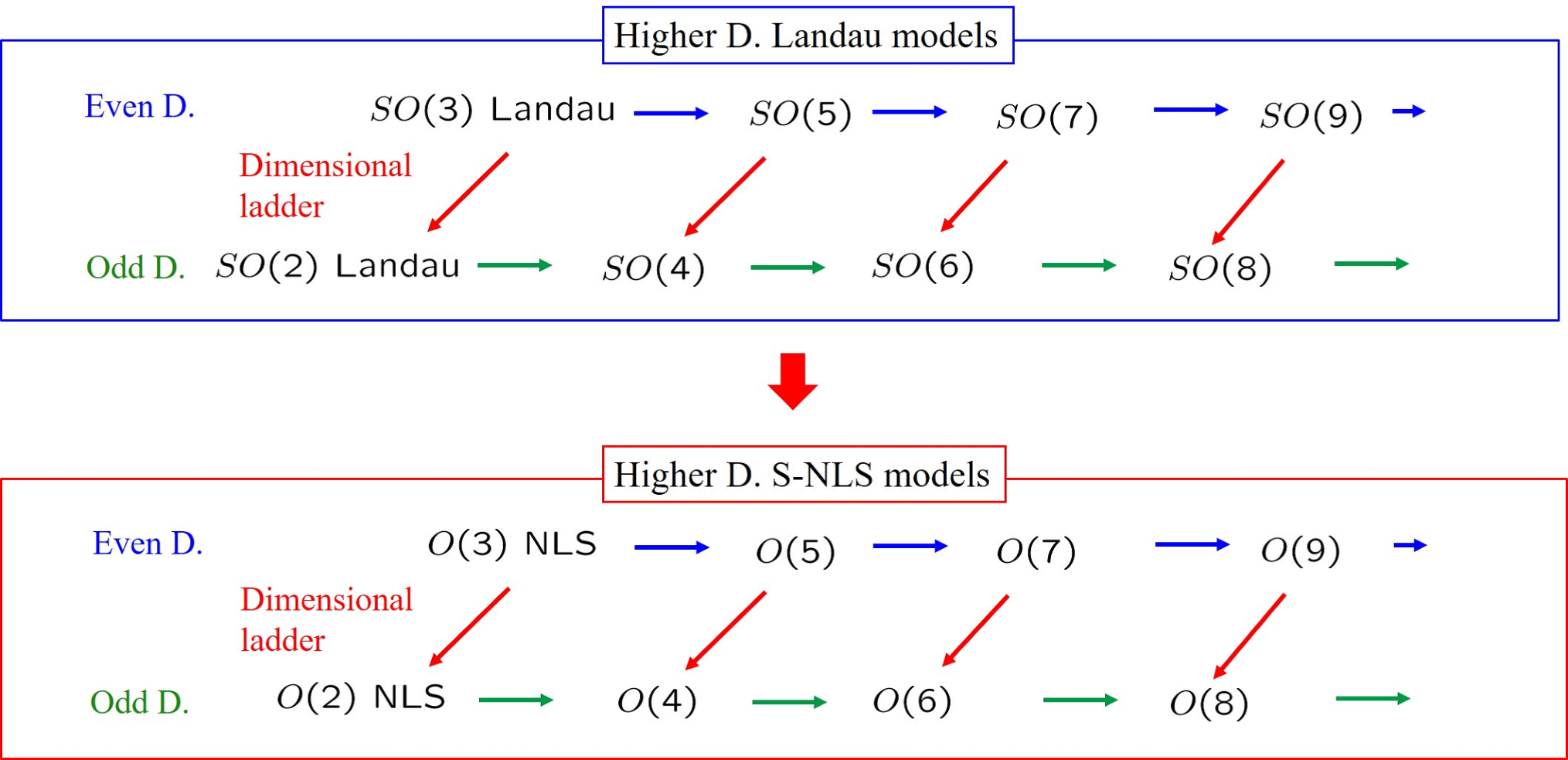
More specifically, the 1D reduction of $H_{2k,2l}$ gives rise to two $O(2k)$ Hamiltonians, $H_{2k-1,2l-1}$ and $H_{2k-1,2l}$ . By removing duplications from the symmetry $H_{2k-1,2l}=H_{2k-1,2k-1-2l}$ , we have $(k-1)$ distinct $O(2k)$ Hamiltonians that exhaust all possible S-NLS model Hamiltonians in $(2k-1)$ D. For instance,¹⁷¹⁷ 17 The soliton configuration of $O(2)$ NLS model is given by the Nielson-Olsen vortex [102].

		$\displaystyle k=2:~~O(5)~\text{S-NLS~model}:~H_{4,2}~~~~~~~~~~~~\rightarrow~~~~~~~O(4)~\text{S-NLS~model}:~H_{3,1},$
		$\displaystyle k=3:~~O(7)~\text{S-NLS~model}:~H_{6,2}~~~~~~~~~~~~\rightarrow~~~~~~~O(6)~\text{S-NLS~model}:~H_{5,1},~~H_{5,2},$
		$\displaystyle k=4:~~O(9)~\text{S-NLS~model}:~H_{8,2},~H_{8,4}~~~~\rightarrow~~~~~~~O(8)~\text{S-NLS~model}:~H_{7,1},~~H_{7,2},~~H_{7,3}.$		(117)

The solitons described by the $O(2k)$ S-NLS model naturally appear as anyonic objects in the BF effective field theory of the odd dimensional quantum Hall effect [69].

5.1 The Chern-Simons term and the action of pure gauge fields

As is well known, the Chern number (density) can be expressed by

\text{tr}(F^{k})=dL_{\text{CS}}^{(2k-1)}[A]

(118)

where $L_{\text{CS}}^{(2k-1)}[A]$ signifies the $(2k-1)$ D Chern-Simons term

L_{\text{CS}}^{(2k-1)}[A]=k\int_{0}^{1}dt~\text{tr}(A(tdA+it^{2}A^{2})^{k-1}).

(119)

In low dimensions, (119) reads as

L_{\text{CS}}^{(1)}[A]=\text{tr}A,~~~~L_{\text{CS}}^{(3)}[A]=\text{tr}(AF-\frac{1}{3}iA^{3}),~~~~L_{\text{CS}}^{(5)}[A]=\text{tr}(AF^{2}-\frac{1}{2}iA^{3}F-\frac{1}{10}A^{5}).

(120)

We make use of the Chern-Simons field description of the Chern number to construct $O(2k)$ S-NLS model Hamiltonians. Recall that the transition function (67) represents $S^{2k-1}_{\text{field}}$ , and the associated gauge field is given by a pure gauge¹⁸¹⁸ 18 $\mathcal{A}$ (121) naturally appears in the context of the hidden local symmetry also (see Appendix D.2).

\mathcal{A}=-ig^{\dagger}dg,~~~~\mathcal{F}=d\mathcal{A}+i\mathcal{A}^{2}=0.

(121)

For the pure gauge (121), the Chern-Simons term (119) is reduced to

	$\displaystyle L_{\text{CS}}^{(2k-1)}[\mathcal{A}]$	$\displaystyle=(-i)^{k-1}\frac{k!(k-1)!}{(2k-1)!}~\text{tr}(\mathcal{A}^{2k-1})$
		$\displaystyle=(-i)^{k-1}\frac{k!(k-1)!}{(2k-1)!}~d^{2k-1}x~\epsilon_{\alpha_{1}\alpha_{2}\cdots\alpha_{2k-1}}\text{tr}(\mathcal{A}_{\alpha_{1}}\mathcal{A}_{\alpha_{2}}\cdots\mathcal{A}_{\alpha_{2k-1}}),$		(122)

where we used $\int_{0}^{1}dt~(t-t^{2})^{k-1}=\frac{((k-1)!)^{2}}{(2k-1)!}$ and assumed that $\mathcal{A}$ is one-form on $x_{\alpha}~\in~\mathbb{R}^{2k-1}_{\text{phys.}}$ :

\mathcal{A}=\sum_{\alpha=1}^{2k-1}\mathcal{A}_{\alpha}dx_{\alpha}.

(123)

We introduce $p$ -rank tensor field associated with the pure gauge as

\mathcal{A}_{\alpha_{1}\alpha_{2}\cdots\alpha_{p}}\equiv(-i)^{\frac{1}{2}p(p-1)}\frac{1}{p!}\mathcal{A}_{[\alpha_{1}}\mathcal{A}_{\alpha_{2}}\cdots\mathcal{A}_{\alpha_{p}]},

(124)

and its dual

	$\displaystyle\tilde{\mathcal{A}}_{\alpha_{1}\alpha_{2}\cdots\alpha_{p}}$	$\displaystyle\equiv\frac{1}{(d-p)!}\epsilon_{\alpha_{1}\alpha_{2}\cdots\alpha_{d}}\mathcal{A}_{\alpha_{p+1}\alpha_{p+2}\cdots\alpha_{d}}$
		$\displaystyle=(-i)^{\frac{1}{2}(d-p)(d-p-1)}\frac{1}{(d-p)!}~\epsilon_{\alpha_{1}\alpha_{2}\cdots\alpha_{d}}\mathcal{A}_{\alpha_{p+1}}\mathcal{A}_{\alpha_{p+2}}\cdots\mathcal{A}_{\alpha_{d}},$		(125)

which satisfies

\frac{1}{p!}{\tilde{\mathcal{A}}_{\alpha_{1}\alpha_{2}\cdots\alpha_{p}}}^{2}=\frac{1}{(2k-1-p)!}{\mathcal{A}_{\alpha_{1}\alpha_{2}\cdots\alpha_{2k-1-p}}}^{2}.

(126)

In (124), $(-i)^{\frac{1}{2}p(p-1)}$ is added so that $\mathcal{A}_{\alpha_{1}\alpha_{2}\cdots\alpha_{p}}$ may be Hermitian. For instance,

		$\displaystyle\mathcal{A}_{\alpha\beta}=-i\frac{1}{2}[\mathcal{A}_{\alpha},\mathcal{A}_{\beta}]=\frac{1}{2}\partial_{[\alpha}\mathcal{A}_{\beta]},$
		$\displaystyle\mathcal{A}_{\alpha\beta\gamma}=i\frac{1}{3!}\mathcal{A}_{[\alpha}\mathcal{A}_{\beta}\mathcal{A}_{\gamma]}=-\frac{1}{3}(\mathcal{A}_{\alpha}\mathcal{A}_{\beta\gamma}+\mathcal{A}_{\beta}\mathcal{A}_{\gamma\alpha}+\mathcal{A}_{\gamma}\mathcal{A}_{\alpha\beta}),$
		$\displaystyle\mathcal{A}_{\alpha\beta\gamma\delta}=-\frac{1}{4!}\mathcal{A}_{[\alpha}\mathcal{A}_{\beta}\mathcal{A}_{\gamma}\mathcal{A}_{\delta]}=\frac{1}{6}(\{\mathcal{A}_{\alpha\beta},\mathcal{A}_{\gamma\delta}\}-\{\mathcal{A}_{\alpha\gamma},\mathcal{A}_{\beta\delta}\}+\{\mathcal{A}_{\alpha\delta},\mathcal{A}_{\beta\gamma}\}).$		(127)

In a similar manner to Sec.4.1, we represent the Chern-Simons action of the pure gauge as¹⁹¹⁹ 19 With $g$ (121) being a non-linear sigma field, (129) becomes the Wess-Zumino action [103] in $(2k-1)$ D: $\Gamma_{\text{WZ}}^{(2k-1)}[g]=\mathcal{S}_{\text{CS}}^{(2k-1)}[\mathcal{A}]\biggr|_{\mathcal{A}=-ig^{\dagger}dg}=-\frac{1}{(2\pi)^{k}}i^{k}\frac{(k-1)!}{(2k-1)!}\int~\text{tr}((g^{\dagger}dg)^{2k-1}).$ (128)

	$\displaystyle\mathcal{S}_{\text{CS}}^{(2k-1)}[\mathcal{A}]$	$\displaystyle\equiv\frac{1}{k!(2\pi)^{k}}\int L_{\text{CS}}^{(2k-1)}[\mathcal{A}]$
		$\displaystyle=\frac{1}{(2\pi)^{k}}\frac{(k-1)!(2k-1-p)!}{(2k-1)!}\int_{\mathbb{R}^{2k-1}_{\text{phys.}}}d^{2k-1}x~\text{tr}(\mathcal{A}_{\alpha_{1}\alpha_{2}\cdots\alpha_{p}}\tilde{\mathcal{A}}_{\alpha_{1}\alpha_{2}\cdots\alpha_{p}}),$		(129)

where

p=1,2,\cdots,k-1.

(130)

In low dimensions, (129) provides

	$\displaystyle\mathcal{S}_{\text{CS}}^{(3)}[\mathcal{A}]$	$\displaystyle=\frac{1}{12\pi^{2}}\int d^{3}x~\text{tr}(\mathcal{A}_{\alpha}\tilde{\mathcal{A}}_{\alpha}),$
	$\displaystyle\mathcal{S}_{\text{CS}}^{(5)}[\mathcal{A}]$	$\displaystyle=\frac{1}{20\pi^{3}}\int d^{5}x~\text{tr}(\mathcal{A}_{\alpha}\tilde{\mathcal{A}}_{\alpha})=\frac{1}{80\pi^{3}}\int d^{5}x~\text{tr}(\mathcal{A}_{\alpha\beta}\tilde{\mathcal{A}}_{\alpha\beta}).$		(131)

From the BPS inequality

S_{2k-1,p}[\mathcal{A}]~\geq~{A}(S^{2k-1})\cdot\mathcal{S}_{\text{CS}}^{(2k-1)}[\mathcal{A}],

(132)

we construct an action made of the pure gauge tensor field:²⁰²⁰ 20 As explained around (29), there exists a local degree of freedom in decomposing $\mathcal{A}_{\alpha_{1}\alpha_{2}\cdots\alpha_{p}}\times\tilde{\mathcal{A}}_{\alpha_{1}\alpha_{2}\cdots\alpha_{p}}$ .

	$\displaystyle{S}_{2k-1,p}[\mathcal{A}]$	$\displaystyle=\frac{1}{2^{k}}\frac{(2k-1-p)!}{(2k-1)!}~\int_{\mathbb{R}^{2k-1}}d^{2k-1}x~\biggl({\text{tr}(\mathcal{A}_{\alpha_{1}\alpha_{2}\cdots\alpha_{p}}}^{2})+\text{tr}({\tilde{\mathcal{A}}_{\alpha_{1}\alpha_{2}\cdots\alpha_{p}}}^{2})\biggr)$
		$\displaystyle=\frac{1}{2^{k}(2k-1)!}~\int_{\mathbb{R}^{2k-1}}d^{2k-1}x~\biggl((2k-1-p)!~\text{tr}({\mathcal{A}_{\alpha_{1}\alpha_{2}\cdots\alpha_{p}}}^{2})+p!~\text{tr}({\mathcal{A}_{\alpha_{p+1}\alpha_{p+2}\cdots\alpha_{2k-1}}}^{2})\biggr).$		(133)

Notice that we can also obtain (133) by the following formal replacement in the $2k$ D tensor gauge field action $S_{2k,2l}$ (80) with the dimensional reduction ( $2k~\rightarrow~2k-1$ ):


$\displaystyle F_{\mu_{1}\mu_{2}\cdots\mu_{2l}},~~~F_{\mu_{2l+1}\mu_{2l+2}\cdots\mu_{2k}}~~~$	$\displaystyle\longrightarrow~~~\mathcal{A}_{\alpha_{1}\alpha_{2}\cdots\alpha_{p=2l-1}},~~~\mathcal{A}_{\alpha_{p+1=2l}\alpha_{p+2}\cdots\alpha_{2k-1}},$	(134a)
	or
$\displaystyle F_{\mu_{1}\mu_{2}\cdots\mu_{2l}},~~~F_{\mu_{2l+1}\mu_{2l+2}\cdots\mu_{2k}}~~~$	$\displaystyle\longrightarrow~~~\mathcal{A}_{\alpha_{1}\alpha_{2}\cdots\alpha_{p=2l}},~~~\mathcal{A}_{\alpha_{p+1=2l+1}\alpha_{p+2}\cdots\alpha_{2k-1}}.$	(134b)

Unlike the $2k$ D action (80), (133) consists of the “bare” tensor gauge fields (not the field strengths), and so $S_{2k-1,p}$ does not have gauge symmetry. Viewing the above process inversely, we may say there always exists one-dimension higher tensor gauge field theory behind every odd D Skyrme model.

5.2 Explicit constructions

With (67), the pure gauge field (121) can be represented as

\mathcal{A}_{\alpha}(n_{m})=-ig^{\dagger}\partial_{\alpha}g=-2\bar{\sigma}_{mn}n_{n}\partial_{\alpha}n_{m},

(135)

where $\bar{\sigma}_{mn}$ denote the $Spin(2k)$ matrix generators. Substituting (135) into (124), we can derive the NLS field expression of $\mathcal{A}_{\alpha_{1}\alpha_{2}\cdots\alpha_{p}}$ . For instance

\mathcal{A}_{\alpha\beta}\biggl|_{\mathcal{A}_{\alpha}=\mathcal{A}_{\alpha}(n_{m})}=-2i\bar{\sigma}_{mp}\bar{\sigma}_{nq}n_{p}n_{q}\partial_{\alpha}n_{[m}\partial_{\beta}n_{n]}=-\bar{\sigma}_{mn}\partial_{\alpha}n_{[n}\partial_{\beta}n_{m]}.

(136)

Just as in the tensor gauge field strength in Sec.4, the antisymmetricity of the $\it{Greek}$ indices of the parent tensor gauge field is inherited to that of the $\it{Latin}$ indices of the NLS field. With such substitutions, the $O(2k)$ S-NLS model Hamiltonian is obtained from $S_{2k-1,p}$ :

		$\displaystyle S_{2k-1,p}~~{\rightarrow}~~$
		$\displaystyle H_{2k-1,p}=\frac{1}{2^{k}(2k-1)!}~\int_{\mathbb{R}^{2k-1}}d^{2k-1}x~\biggl((2k-1-p)!~\text{tr}({\mathcal{A}_{\alpha_{1}\alpha_{2}\cdots\alpha_{p}}}^{2})+p!~\text{tr}({\mathcal{A}_{\alpha_{1}\alpha_{2}\cdots\alpha_{2k-1-p}}}^{2})\biggr)\biggl\|_{{\mathcal{A}_{\alpha}=\mathcal{A}_{\alpha}(n_{m})}}.$		(137)

Similarly, the Chern-Simons term (129) turns to the winding number of $\pi_{2k-1}(S^{2k-1})\simeq\mathbb{Z}$ :

\displaystyle\mathcal{S}_{\text{CS}}^{(2k-1)}~~{\rightarrow}~~N_{2k-1}=\frac{1}{{A}(S^{2k-1})}\int_{\mathbb{R}^{2k-1}_{\text{phys.}}}d^{2k-1}x~\epsilon_{m_{1}m_{2}\cdots m_{2k}}n_{m_{2k}}\partial_{1}n_{m_{1}}\partial_{2}n_{m_{2}}\cdots\partial_{{2k-1}}n_{m_{2k-1}}.

(138)

As in the previous $O(2k+1)$ S-NLS models, the parent BPS inequality (132) guarantees the BPS inequality of the $O(2k)$ S-NLS models:

H_{2k-1,p}~\geq~{A}(S^{2k-1})\cdot N_{2k-1}.

(139)

Since the parent pure actions (133) do not have gauge symmetries, the corresponding $O(2k)$ S-NLS models do not either. This “explains” the non-existence of the gauge symmetry of the Skyrme models in odd dimensions. In the following, we demonstrate the above procedure to derive the $O(2k)$ S-NLS model Hamiltonians for $d=3$ and $d=5$ .

5.2.1 The Skyrme model: $O(4)$ S-NLS model

For $d=3$ , the pure gauge field action is given by

S_{3,1}=\frac{1}{12}\int_{\mathbb{R}_{\text{phys.}}^{3}}d^{3}x~\text{tr}({\mathcal{A}_{\alpha}}^{2}+{\tilde{\mathcal{A}}_{\alpha}}^{2})=\frac{1}{12}\int_{\mathbb{R}_{\text{phys.}}^{3}}d^{3}x~(\text{tr}({\mathcal{A}_{\alpha}}^{2})+\frac{1}{2}\text{tr}({\mathcal{A}_{\alpha\beta}}^{2}))=S_{3,2},

(140)

where $\mathcal{A}_{\alpha}$ and its dual field $\tilde{\mathcal{A}}_{\alpha}$ are represented as

\mathcal{A}_{\alpha}=2\bar{\sigma}_{mn}n_{m}\partial_{\alpha}n_{n},~~~~\tilde{\mathcal{A}}_{\alpha}=\frac{1}{2}\epsilon_{\alpha\beta\gamma}A_{\beta\gamma}=\epsilon_{\alpha\beta\gamma}\bar{\sigma}_{mn}\partial_{\beta}n_{m}\partial_{\gamma}n_{n},

(141)

with $Spin(4)$ matrix generators:

\bar{\sigma}_{mn}=\frac{1}{2}\bar{\eta}_{mn}^{i}\sigma_{i}.

(142)

From the following formula²¹²¹ 21 The $U(2)$ generators (the Pauli matrices and the unit matrix) span the $2\times 2$ matrix space, and so the product of two $SU(2)$ Pauli matrices or $Spin(4)$ matrix generators can be represented as a linear combination of the $U(2)$ generators.

\bar{\sigma}_{mn}\bar{\sigma}_{pq}=\frac{1}{4}(\delta_{mp}\delta_{nq}-\delta_{mq}\delta_{np}-\epsilon_{mnpq})1_{2}+i\frac{1}{2}(\delta_{mp}\bar{\sigma}_{nq}-\delta_{mq}\bar{\sigma}_{np}+\delta_{nq}\bar{\sigma}_{mp}-\delta_{np}\bar{\sigma}_{mq}),

(143)

we can readily show

\text{tr}({\mathcal{A}_{\alpha}}^{2})|_{\mathcal{A}=\mathcal{A}(n_{m})}=2(\partial_{\alpha}n_{m})^{2},~~~~~~\text{tr}({\tilde{\mathcal{A}}_{\alpha}}^{2})|_{\mathcal{A}=\mathcal{A}(n_{m})}=\frac{1}{2}(\partial_{\alpha}n_{[m}\partial_{\beta}n_{n]})^{2}

(144)

to have

H_{3,1}=\frac{1}{6}\int_{\mathbb{R}_{\text{phys.}}^{3}}d^{3}x~\biggl((\partial_{\alpha}n_{m})^{2}+\frac{1}{4}(\partial_{\alpha}n_{[m}\partial_{\beta}n_{n]})^{2}\biggr).

(145)

Thus, the $O(4)$ S-NLS model Hamiltonian is nothing but the original Skyrme Hamiltonian. As mentioned before, the anti-symmetricity of the indices of $\mathcal{A}_{\alpha\beta}$ is inherited to the anti-symmetricity of the Latin indices of $O(4)$ NLS field of the Skyrme term.

5.2.2 $O(6)$ S-NLS models

Next we consider the case $d=5$ . There exist two distinct actions:


$\displaystyle S_{5,1}$	$\displaystyle=\frac{1}{40}\int_{\mathbb{R}^{5}_{\text{phys.}}}d^{5}x~\text{tr}({\mathcal{A}_{\alpha}}^{2}+{\tilde{\mathcal{A}}_{\alpha}}^{2})=\frac{1}{40}\int_{\mathbb{R}^{5}_{\text{phys.}}}d^{5}x~\text{tr}({\mathcal{A}_{\alpha}}^{2}+\frac{1}{4!}{{\mathcal{A}}_{\alpha\beta\gamma\delta}}^{2}),$	(146a)
$\displaystyle S_{5,2}$	$\displaystyle=\frac{1}{160}\int_{\mathbb{R}^{5}_{\text{phys.}}}d^{5}x~\text{tr}({\mathcal{A}_{\alpha\beta}}^{2}+{\tilde{\mathcal{A}}_{\alpha\beta}}^{2})=\frac{1}{160}\int_{\mathbb{R}^{5}_{\text{phys.}}}d^{5}x~\text{tr}({\mathcal{A}_{\alpha\beta}}^{2}+\frac{1}{3}{\mathcal{A}_{\alpha\beta\gamma}}^{2}),$	(146b)

$\mathcal{A}_{\alpha}$ is given by (135) with $Spin(6)$ matrix generators $\bar{\sigma}_{mn}$ . From the isomorphism $Spin(6)\simeq SU(4)$ , we can express the $Spin(6)$ matrices $\bar{\sigma}_{mn}$ as a linear combination of the $SU(4)$ Gell-Mann matrices $\lambda_{A=1,2,\cdots,15}$ [104]:

\bar{\sigma}_{mn}=\frac{1}{2}\sum_{A=1}^{15}\bar{\eta}_{mn}^{A}\lambda_{A}.

(147)

Here we introduced an $SU(4)$ -generalized ’t Hooft symbol, $\bar{\eta}_{mn}^{A}=\text{tr}(\lambda_{A}\bar{\sigma}_{mn})$ (see Appendix B.2 for detail properties). The product of two $Spin(6)$ generators is explicitly given by²²²² 22 The $SU(4)$ Gell-Mann matrices [104] are ortho-normalized as $\text{tr}(\lambda_{A}\lambda_{B})=2\delta_{AB}$ , and with the $4\times 4$ unit matrix they constitute the $U(4)$ matrix generators that span the whole $4\times 4$ matrix space.

\bar{\sigma}_{mn}\bar{\sigma}_{pq}=\frac{1}{4}(\delta_{mp}\delta_{nq}-\delta_{mq}\delta_{nq})1_{4}+i\frac{1}{2}(\delta_{mp}\bar{\sigma}_{nq}-\delta_{mq}\bar{\sigma}_{np}+\delta_{nq}\bar{\sigma}_{mp}-\delta_{np}\bar{\sigma}_{mq})-\frac{1}{4}\epsilon_{mnpqrs}\bar{\sigma}_{rs}.

(148)

From this formula, the pure tensor gauge fields can be expressed as

		$\displaystyle\mathcal{A}_{\alpha\beta}=-\bar{\sigma}_{mn}\partial_{\alpha}n_{[n}\partial_{\beta}n_{m]},$
		$\displaystyle\mathcal{A}_{\alpha\beta\gamma}=-\frac{1}{3}(\mathcal{A}_{\alpha\beta}\mathcal{A}_{\gamma}+\mathcal{A}_{\beta\gamma}\mathcal{A}_{\alpha}+\mathcal{A}_{\rho\mu}A_{\nu})=\epsilon_{mnpqrs}\partial_{\alpha}n_{m}\partial_{\beta}n_{n}\partial_{\gamma}n_{p}n_{q}\bar{\sigma}_{rs},$
		$\displaystyle\mathcal{A}_{\alpha\beta\gamma\delta}=\frac{1}{3!}(\{\mathcal{A}_{\alpha\beta},\mathcal{A}_{\gamma\delta}\}-\{\mathcal{A}_{\alpha\gamma},\mathcal{A}_{\beta\delta}\}+\{\mathcal{A}_{\alpha\delta},\mathcal{A}_{\beta\gamma}\})=-\epsilon_{mnpqrs}\bar{\sigma}_{rs}\partial_{\alpha}n_{m}\partial_{\beta}n_{n}\partial_{\gamma}n_{p}\partial_{\delta}n_{q},$		(149)

where we used

		$\displaystyle\mathcal{A}_{\alpha\beta}\mathcal{A}_{\gamma}=2in_{p}\bar{\sigma}_{mp}\partial_{\gamma}n_{n}(\partial_{\alpha}n_{m}\partial_{\beta}n_{n}-\partial_{\beta}n_{m}\partial_{\alpha}n_{n})-\epsilon_{mnpqrs}\partial_{\alpha}n_{m}\partial_{\beta}n_{n}\partial_{\gamma}n_{q}n_{p}\bar{\sigma}_{rs},$
		$\displaystyle\{\mathcal{A}_{\alpha\beta},\mathcal{A}_{\gamma\delta}\}=2(\partial_{\alpha}n_{m}\partial_{\gamma}n_{m}\cdot\partial_{\beta}n_{n}\partial_{\delta}n_{n}-\partial_{\alpha}n_{m}\partial_{\delta}n_{m}\cdot\partial_{\beta}n_{n}\partial_{\gamma}n_{n})1_{4}-2\epsilon_{mnpqrs}\partial_{\alpha}n_{m}\partial_{\beta}n_{n}\partial_{\rho}n_{p}\partial_{\sigma}n_{r}\bar{\sigma}_{rs}.$		(150)

Substituting (149) into (146), we obtain the $O(6)$ S-NLS model Hamiltonians:


$\displaystyle H_{5,1}$	$\displaystyle=\frac{1}{10}\int_{\mathbb{R}^{5}_{\text{phys.}}}d^{5}x~\biggl((\partial_{\alpha}n_{m})^{2}+\frac{1}{(4!)^{2}}(\partial_{\alpha}n_{[m}\partial_{\beta}n_{n}\partial_{\gamma}n_{p}\partial_{\delta}n_{q]})^{2}\biggr),$	(151a)
$\displaystyle H_{5,2}$	$\displaystyle=\frac{1}{80}\int_{\mathbb{R}^{5}_{\text{phys.}}}d^{5}x~\biggl((\partial_{\alpha}n_{[m}\partial_{\beta}n_{n]})^{2}+\frac{1}{9}~(\partial_{\alpha}n_{[m}\partial_{\beta}n_{n}\partial_{\gamma}n_{p]})^{2}\biggr).$	(151b)

The octic derivative term of $H_{5,1}$ is similarly given by (95) and the sextic derivative term of $H_{5,2}$ is

(\partial_{\alpha}n_{[m}\partial_{\beta}n_{n}\partial_{\gamma}n_{p]})^{2}=6((\partial_{\alpha}n_{m})^{2})^{3}-18(\partial_{\alpha}n_{m})^{2}(\partial_{\beta}n_{n}\partial_{\gamma}n_{p})^{2}+12(\partial_{\alpha}n_{m}\partial_{\beta}n_{m})(\partial_{\beta}n_{n}\partial_{\gamma}n_{n})(\partial_{\gamma}n_{p}\partial_{\alpha}n_{p}).

(152)

$H_{5,1}$ and $H_{5,2}$ respectively correspond to the Type I and Type II Skyrme Hamiltonians on $S^{5}$ [100].

The mathematical structure of the $O(6)$ S-NLS model Hamiltonians is quite similar to that of the Skyrme’s $O(4)$ Hamiltonian (145). Each partial derivative acts to every component of the NLS field and all of the Latin indices of the components are totally antisymmetrized to build the constituent terms of the Hamiltonian. Recall that the $O(2k+1)$ S-NLS model Hamiltonians exhibited the similar structures. Such common structures between $O(2k+1)$ and $O(2k)$ S-NLS models suggest an existence of a unified formulation that covers all of the S-NLS models. We shall explore the formulation in Sec.6.

As a final comment of this section, we mention about relationship to the formerly derived 7(+1)D Skyrmion model by the Atiyah-Manton construction [39]. For $k=4$ and $p=3$ , (137) yields an $O(8)$ S-NLS Hamiltonian:

H_{7,3}=\frac{1}{3360}\int_{\mathbb{R}^{7}}d^{7}x~\text{tr}(\mathcal{A}_{\alpha\beta\gamma}^{2}+\tilde{\mathcal{A}}_{\alpha\beta\gamma}^{2})=\frac{1}{3360}\int_{\mathbb{R}^{7}}d^{7}x~\text{tr}(\mathcal{A}_{\alpha\beta\gamma}^{2}+\frac{1}{4}{\mathcal{A}}_{\alpha\beta\gamma\delta}^{2}).

(153)

Interestingly, (153) takes the same form as the 7D Skyrme Hamiltonian obtained in [39]. Although detail relations between the present and Atiyah-Manton constructions need to be excavated, both of them are based on the hierarchical construction from instantons and practically apply the replacement (134) to the gauge theory actions to yield same Skyrme Hamiltonians.

6 $O(d+1)$ S-NLS Models

We discuss a general construction of the S-NLS models from the expression of higher winding number. This construction actually reproduces all of the S-NLS model Hamiltonians previously derived and also supplements other S-NLS model Hamiltonians of the type $H_{2k,\text{odd}}$ in even D that eluded the previous discussions based on the tensor gauge theories.

6.1 $O(d+1)$ S-NLS models and their basic properties

6.1.1 General $O(d+1)$ S-NLS model Hamiltonians

The winding number of the $O(d+1)$ NLS model associated with

\pi_{d}(S^{d})\simeq\mathbb{Z}

(154)

is given by [101]

	$\displaystyle N_{d}$	$\displaystyle=\frac{1}{{A}(S^{d}_{\text{phys.}})}~\frac{1}{d!}\int_{\mathbb{R}^{d}_{\text{phys.}}}d^{d}x~\epsilon_{a_{1}a_{2}\cdots a_{d+1}}\epsilon_{\mu_{1}\mu_{2}\cdots\mu_{d}}n_{a_{d+1}}\partial_{\mu_{1}}n_{a_{1}}\partial_{\mu_{2}}n_{a_{2}}\cdots\partial_{\mu_{d}}n_{a_{d}}$
		$\displaystyle=\frac{1}{{A}(S^{d}_{\text{phys.}})}~\int_{\mathbb{R}^{d}_{\text{phys.}}}d^{d}x~\epsilon_{a_{1}a_{2}\cdots a_{d+1}}n_{a_{d+1}}\partial_{1}n_{a_{1}}\partial_{2}n_{a_{2}}\cdots\partial_{d}n_{a_{d}},$		(155)

where $n_{a}(x)$ denote the $O(d+1)$ NLS model field on $x_{\mu}\in\mathbb{R}^{d}$ subject to

\sum_{a=1}^{d+1}n_{a}n_{a}=1~:~S^{d}.

(156)

As in the previous cases, we first decompose the winding number (155) as

N_{d}=\frac{1}{\mathcal{A}({S^{d}})}\frac{p!(d-p)!}{d!}\int_{\mathbb{R}^{d}}d^{d}x~N^{a_{1}a_{2}\cdots a_{p}}_{\mu_{1}\mu_{2}\cdots\mu_{p}}~\tilde{N}^{a_{1}a_{2}\cdots a_{p}}_{\mu_{1}\mu_{2}\cdots\mu_{p}}

(157)

where


$\displaystyle N^{a_{1}a_{2}\cdots a_{p}}_{\mu_{1}\mu_{2}\cdots\mu_{p}}$	$\displaystyle\equiv\frac{1}{p!}\partial_{\mu_{1}}n_{[a_{1}}\partial_{\mu_{2}}n_{a_{2}}\cdots\partial_{\mu_{p}}n_{a_{p}]},$	(158a)
$\displaystyle\tilde{N}^{a_{1}a_{2}\cdots a_{p}}_{\mu_{1}\mu_{2}\cdots\mu_{p}}$	$\displaystyle\equiv\frac{1}{p!(d-p)!}\epsilon_{\mu_{1}\mu_{2}\cdots\mu_{d}}\epsilon_{a_{1}a_{2}\cdots a_{d+1}}n_{a_{d+1}}N_{\mu_{p+1}\mu_{p+2}\cdots\mu_{d}}^{a_{p+1}a_{p+2}\cdots a_{d}}$
	$\displaystyle=\frac{1}{p!(d-p)!}\epsilon_{\mu_{1}\mu_{2}\cdots\mu_{d}}\epsilon_{a_{1}a_{2}\cdots a_{d+1}}n_{a_{d+1}}\partial_{\mu_{p+1}}n_{a_{p+1}}\partial_{\mu_{p+2}}n_{a_{p+2}}\cdots\partial_{\mu_{d}}n_{a_{d}}.$	(158b)

The BPS inequality, $(N^{a_{1}a_{2}\cdots a_{p}}_{\mu_{1}\mu_{2}\cdots\mu_{p}}-\tilde{N}^{a_{1}a_{2}\cdots a_{p}}_{\mu_{1}\mu_{2}\cdots\mu_{p}})^{2}\geq 0$ , or

H_{d,p}\geq{A}(S^{d})\cdot N_{d},

(159)

yields the $O(d+1)$ S-NLS model Hamiltonian:

H_{d,p}=H_{d,p}^{(1)}+H_{d,p}^{(2)}

(160)

with


		$\displaystyle H_{d,p}^{(1)}=\frac{(d-p)!}{2~d!p!}\int_{\mathbb{R}_{\text{phys.}}^{d}}d^{d}x~~(\partial_{\mu_{1}}n_{[a_{1}}\partial_{\mu_{2}}n_{a_{2}}\cdots\partial_{\mu_{p}}n_{a_{p}]})^{2},$		(161a)
		$\displaystyle H_{d,p}^{(2)}=\frac{p!}{2~d!(d-p)!}\int_{\mathbb{R}_{\text{phys.}}^{d}}d^{d}x~(\partial_{\mu_{1}}n_{[a_{1}}\partial_{\mu_{2}}n_{a_{2}}\cdots\partial_{\mu_{d-p}}n_{a_{d-p}]})^{2}.$		(161b)

The BPS equation, ${N_{\mu_{1}\mu_{2}\cdots\mu_{p}}^{a_{1}a_{2}\cdots a_{p}}}={\tilde{N}_{\mu_{1}\mu_{2}\cdots\mu_{p}}^{a_{1}a_{2}\cdots a_{p}}}$ , is rephrased as

\partial_{\mu_{1}}n_{[a_{1}}\partial_{\mu_{2}}n_{a_{2}}\cdots\partial_{\mu_{p}}n_{a_{p}]}=\frac{1}{(d-p)!}\epsilon_{\mu_{1}\mu_{2}\cdots\mu_{d}}\epsilon_{a_{1}a_{2}\cdots a_{d+1}}n_{a_{d+1}}\partial_{\mu_{p+1}}n_{a_{p+1}}\partial_{\mu_{p+2}}n_{a_{p+2}}\cdots\partial_{\mu_{d}}n_{a_{d}}.

(162)

Notice that the $O(d+1)$ Hamiltonian is invariant under the interchange $p~\leftrightarrow~d-p$ :

H_{d,p}=H_{d,d-p}.

(163)

Therefore, there are $[d/2]$ distinct Hamiltonians in correspondence with $p=1,2,\cdots[d/2]$ . One may readily check that (160) reproduces the $O(2k+1)$ S-NLS model Hamiltonians, (101) and (116), and also the $O(2k)$ S-NLS model Hamiltonians, (145) and (151). Not only do $H_{d,p}$ cover all of the previously derived S-NLS model Hamiltonians, but $H_{d,p}$ also provide other S-NLS model Hamiltonians that eluded the previous derivations. In low dimensions, from (160) such S-NLS model Hamiltonians are obtained as

		$\displaystyle H_{2,1}=\frac{1}{2}\int_{\mathbb{R}^{2}_{\text{phys.}}}d^{2}x~(\partial_{\mu}n_{a})^{2},$
		$\displaystyle H_{4,1}=\frac{1}{8}\int_{\mathbb{R}^{4}_{\text{phys.}}}d^{4}x~\biggl((\partial_{\mu}n_{a})^{2}+\frac{1}{36}(\partial_{\mu}n_{[b}\partial_{\nu}n_{c}\partial_{\rho}n_{d]})^{2}\biggr),$
		$\displaystyle H_{6,1}=\frac{1}{12}\int_{\mathbb{R}^{6}_{\text{phys.}}}d^{6}x~\biggl((\partial_{\mu}n_{a})^{2}+\frac{1}{14400}(\partial_{\mu_{1}}n_{[a_{1}}\partial_{\mu_{2}}n_{a_{2}}\cdots\partial_{\mu_{5}}n_{a_{5}]})^{2}\biggr),$
		$\displaystyle H_{6,3}=\frac{1}{720}\int_{\mathbb{R}^{6}_{\text{phys.}}}d^{6}x~(\partial_{\mu_{1}}n_{[a_{1}}\partial_{\mu_{2}}n_{a_{2}}\cdots\partial_{\mu_{6}}n_{a_{6}]})^{2}.$		(164)

Note that $H_{2,1}$ represents the well known $O(3)$ NLS model Hamiltonian.

It is not difficult also to incorporate non-derivative term ( $p=0$ ) in the present formalism. With

H_{d,p=0}^{(1)}=\frac{1}{2}\int_{\mathbb{R}_{\text{phys.}}^{d}}d^{d}x~U(n),~~~~~~H_{d,p}^{(2)}=\frac{1}{2~{d!}^{2}}\int_{\mathbb{R}_{\text{phys.}}^{d}}d^{d}x~(\partial_{\mu_{1}}n_{[a_{1}}\partial_{\mu_{2}}n_{a_{2}}\cdots\partial_{\mu_{d}}n_{a_{d}]})^{2},

(165)

we have

H_{d,p=0}=\frac{1}{2}\int_{\mathbb{R}_{\text{phys.}}^{d}}d^{d}x\biggl(\frac{1}{{d!}^{2}}~(\partial_{\mu_{1}}n_{[a_{1}}\partial_{\mu_{2}}n_{a_{2}}\cdots\partial_{\mu_{d}}n_{a_{d}]})^{2}+U(n)\biggr),

(166)

which is exactly equal to the Hamiltonian introduced in [105]. The BPS inequality is given by

H_{d,p=0}~\geq~\frac{1}{d!}\int_{\mathbb{R}_{\text{phys.}}^{d}}d^{d}x~\epsilon_{\mu_{1}\mu_{2}\cdots\mu_{d}}\epsilon^{a_{1}a_{2}\cdots a_{d+1}}\sqrt{U(n)}~n_{a_{d+1}}\partial_{\mu_{1}}n_{a_{1}}\partial_{\mu_{2}}n_{a_{2}}\cdots\partial_{\mu_{d}}n_{a_{d}}.

(167)

For $U=1$ , the right-hand side of (167) is reduced to the usual topological number $A(S^{d})\cdot N_{d}$ . (166) realizes the restricted baby Skyrme model for $d=2$ [106, 107, 108] and the BPS Skyrme model for $d=3$ [109, 110].²³²³ 23 Recently, BPS Skyrme models attracted much attention for the reason that they can lower the binding energy compared to the original Skyrme model [111, 112, 113, 114].

6.1.2 Equations of motion and the scaling arguments

From (160), it is not difficult to derive the equations of motion:

		$\displaystyle\partial_{\mu_{1}}\biggl((d-p-1)!~\partial_{\mu_{2}}n_{a_{2}}\partial_{\mu_{3}}n_{a_{3}}\cdots\partial_{\mu_{p}}n_{a_{p}}\cdot\partial_{\mu_{1}}n_{[a_{1}}\partial_{\mu_{2}}n_{a_{2}}\partial_{\mu_{3}}n_{a_{3}}\cdots\partial_{\mu_{p}}n_{a_{p}]}$
		$\displaystyle~~~+(p-1)!~\partial_{\mu_{2}}n_{a_{2}}\partial_{\mu_{3}}n_{a_{3}}\cdots\partial_{\mu_{d-p}}n_{a_{d-p}}\cdot\partial_{\mu_{1}}n_{[a_{1}}\partial_{\mu_{2}}n_{a_{2}}\partial_{\mu_{3}}n_{a_{3}}\cdots\partial_{\mu_{d-p}}n_{a_{d-p}]}\biggr)-\lambda n_{a_{1}}=0,$		(168)

where $\lambda$ denotes the Lagrange multiplier

	$\displaystyle\lambda=n_{a_{1}}\partial_{\mu_{1}}$	$\displaystyle\biggl((d-p-1)!~\partial_{\mu_{2}}n_{a_{2}}\partial_{\mu_{3}}n_{a_{3}}\cdots\partial_{\mu_{p}}n_{a_{p}}\cdot\partial_{\mu_{1}}n_{[a_{1}}\partial_{\mu_{2}}n_{a_{2}}\partial_{\mu_{3}}n_{a_{3}}\cdots\partial_{\mu_{p}}n_{a_{p}]}$
		$\displaystyle+(p-1)!~\partial_{\mu_{2}}n_{a_{2}}\partial_{\mu_{3}}n_{a_{3}}\cdots\partial_{\mu_{d-p}}n_{a_{d-p}}\cdot\partial_{\mu_{1}}n_{[a_{1}}\partial_{\mu_{2}}n_{a_{2}}\partial_{\mu_{3}}n_{a_{3}}\cdots\partial_{\mu_{d-p}}n_{a_{d-p}]}\biggr).$		(169)

For $(d,p)=(2k,2l)$ , (168) signifies the equations of motion of the $O(2k+1)$ S-NLS model Hamiltonian (83). In particular for $(d,p)=(2k,2)$ , (168) becomes

\partial_{\mu_{1}}\biggl(\partial_{\mu_{2}}n_{b}\cdot\partial_{\mu_{1}}{n}_{[a}\partial_{\mu_{2}}{n}_{b]}+\frac{1}{(2k-3)!}~\partial_{\mu_{2}}{n}_{a_{2}}\cdots\partial_{\mu_{2k-2}}{n}_{a_{2k-2}}~\cdot~\partial_{\mu_{1}}{n}_{[a}\partial_{\mu_{2}}n_{a_{2}}\cdots\partial_{\mu_{2k-2}}{n}_{{a_{2k-2}}]}\biggr)-\frac{1}{(2k-3)!}\lambda n_{a}=0,

(170)

which represents the equations of motion of (101). In low dimensions, (168) gives

		$\displaystyle(d,p)=(2,1)~:~2{\partial_{\mu}}^{2}n_{a}-\lambda n_{a}=0,$
		$\displaystyle(d,p)=(3,1)~:~1!~{\partial_{\mu}}^{2}n_{a}+\partial_{\mu}(\partial_{\nu}n_{b}\partial_{\mu}n_{[a}\partial_{\nu}n_{b]})-\lambda n_{a}=0,$
		$\displaystyle(d,p)=(4,1)~:~2!~{\partial_{\mu}}^{2}n_{a}+\partial_{\mu}(\partial_{\nu}n_{n}\partial_{\rho}n_{p}\partial_{\mu}n_{[a}\partial_{\nu}n_{b}\partial_{\rho}n_{c]})-\lambda n_{a}=0,$
		$\displaystyle(d,p)=(4,2)~:~2\partial_{\mu}(\partial_{\nu}n_{b}\partial_{\mu}n_{[a}\partial_{\nu}n_{b]})-\lambda n_{a}=0,$
		$\displaystyle(d,p)=(5,1)~:~3!~{\partial_{\mu}}^{2}n_{a}+\partial_{\mu}(\partial_{\nu}n_{b}\partial_{\rho}n_{c}\partial_{\sigma}n_{d}\partial_{\mu}n_{[a}\partial_{\nu}n_{b}\partial_{\rho}n_{c}\partial_{\sigma}n_{d]})-\lambda n_{a}=0,$
		$\displaystyle(d,p)=(5,2)~:~2\partial_{\mu}(\partial_{\nu}n_{b}\partial_{\mu}n_{[a}\partial_{\nu}n_{b]})+\partial_{\mu}(\partial_{\nu}n_{b}\partial_{\rho}n_{c}\partial_{\mu}n_{[a}\partial_{\nu}n_{b}\partial_{\rho}n_{c]})-\lambda n_{a}=0.$		(171)

The equations of motion of the $O(3)$ NLS model and the $O(5)$ S-NLS model are realized for $(d,p)=(2,1)$ and $(4,2)$ in (171), respectively. For the $O(3)$ NLS model, soliton solutions with arbitrary winding number are derived in [56, 57], but for other S-NLS models, to solve the equations of motion (168) is rather formidable in general.

Instead of solving the equations of motion, we prepare one(-scale)-parameter family of field configurations and evaluate the size of the configuration based on the scaling argument of Derrick [115]. The mass dimensions of the quantities inside the integrals of $H_{d,p}^{(1)}$ and $H_{d,p}^{(2)}$ (161) are $2p-d$ and $d-2p$ , respectively.²⁴²⁴ 24 Both $H_{d,p}^{(1)}$ and $H_{d,p}^{(2)}$ should have mass dimension one, and so, to be precise, some dimensionful parameters are necessary in front of them to adjust the dimension counting. Suppose that the energy of a given field configuration $n_{a}(x)$ is given by $E_{d,p}=E_{d,p}^{(1)}+E_{d,p}^{(2)}$ . Under the scale transformation

n_{a}(x)~\rightarrow~n^{(R)}_{a}(x)\equiv n_{a}(x/{R}),

(172)

$E_{d,p}^{(1)}$ and $E_{d,p}^{(2)}$ are transformed as

E_{d,p}=E_{d,p}^{(1)}+E_{d,p}^{(2)}~\rightarrow~E_{d,p}(R)=E_{d,p}^{(1)}(R)+E_{d,p}^{(2)}(R),

(173)

where

E_{d,p}^{(1)}(R)={R^{d-2p}}E_{d,p}^{(1)},~~~E_{d,p}^{(2)}(R)=\frac{1}{R^{d-2p}}E_{d,p}^{(2)}.

(174)

The scale parameter $R$ can be considered as a variational parameter that represents the size of the field configuration. For $p>[d/2]$ , as $R$ increases, $E_{d,p}^{(1)}(R)$ monotonically increases while $E_{d,p}^{(2)}(R)$ monotonically decreases. This implies that $E_{d,p}^{(1)}(R)$ term energetically favors a smaller size field configuration while $E_{d,p}^{(2)}(R)$ favors a larger size configuration. These two competing effects determine an optimal size of the field configuration of soliton. More specifically, we take the derivative of $E_{d,p}(R)$ (173) with respect to $R$ to obtain a local energy minimum and have

\bar{R}_{d,p}=\biggl(\frac{E^{(2)}_{d,p}}{E_{d,p}^{(1)}}\biggr)^{\frac{1}{2(d-2p)}}.

(175)

The present S-NLS models thus realize soliton configurations with the finite size (175) (except for the scale invariant case $P=[d/2]$ ), and two competing energies are exactly balanced at the point:

E_{d,p}^{(1)}(\bar{R})=(E_{d,p}^{(1)}E_{d,p}^{(2)})^{\frac{1}{2(d-2p)}}=E_{d,p}^{(2)}(\bar{R}),

(176)

which signifies the virial relation in higher dimensions.

6.1.3 Scale invariant solutions

Next let us consider $(d,p)=(2k,k)$ , in which the two competing Hamiltonians coincide, $H_{2k,k}^{(1)}=H_{2k,k}^{(2)}$ , to realize scale invariant field solutions.²⁵²⁵ 25 Other types of scale invariant solitons associated with the Hopf map are proposed in [116, 117] and [118]. The S-NLS model Hamiltonian (160) becomes

H_{2k,k}=\frac{1}{(2k)!}\int_{\mathbb{R}^{d}}d^{d}x~(\partial_{\mu_{1}}n_{[a_{1}}\partial_{\mu_{2}}n_{a_{2}}\cdots\partial_{\mu_{p}}n_{a_{k}]})^{2}.

(177)

When $k$ is even, (177) is exactly equal to the former scale invariant Hamiltonian (116). The equations of motion (168) and the BPS equation (162) are reduced to


		$\displaystyle\partial_{\mu_{1}}\biggl((\partial_{\mu_{2}}n_{a_{2}}\cdots\partial_{\mu_{p}}n_{a_{k}})\cdot(\partial_{\mu_{1}}n_{[a_{1}}\partial_{\mu_{2}}n_{a_{2}}\cdots\partial_{\mu_{k}}n_{a_{k}]})\biggr)-\frac{1}{2(k-1)!}\lambda n_{a_{1}}=0,$		(178a)
		$\displaystyle\partial_{\mu_{1}}n_{[a_{1}}\partial_{\mu_{2}}n_{a_{2}}\cdots\partial_{\mu_{k}}n_{a_{k}]}-\frac{1}{k!}\epsilon_{\mu_{1}\mu_{2}\cdots\mu_{2k}}\epsilon_{a_{1}a_{2}\cdots a_{2k+1}}n_{a_{2k+1}}\partial_{\mu_{k+1}}n_{a_{k+1}}\partial_{\mu_{k+2}}n_{a_{k+2}}\cdots\partial_{\mu_{2k}}n_{a_{2k}}=0.$		(178b)

Especially for $d=4$ , (178a) reproduces the $(d,p)=(4,2)$ equation of (171). The equations of motion (178a) are highly non-linear equations, but the inverse stereographic coordinate configuration

n_{a}(x)=r_{a}\equiv\{\frac{2}{1+x^{2}}x_{\mu},\frac{1-x^{2}}{1+x^{2}}\},

(179)

realizes a simple solution of (178a) and satisfies the BPS equation (178b) also.²⁶²⁶ 26 Also recall the results of Sec.4.3.2 where the tensor instanton configuration satisfies the BPS equation and the equations of motion. From the one-to-one correspondence between the points on $\mathbb{R}^{2k}$ and those on $S^{2k}$ , it may be obvious that (179) also represents a field configuration of the winding number 1. One can explicitly confirm this as

N_{d}|_{n_{a}=r_{a}}=\frac{1}{A(S^{d})}\int_{\mathbb{R}_{\text{phys.}}^{d}}d^{d}x~\epsilon_{a_{1}a_{2}\cdots a_{d+1}}r_{a_{d+1}}\partial_{1}r_{a_{1}}\partial_{2}r_{a_{2}}\cdots\partial_{d}r_{a_{d}}=\frac{A(S^{d-1})}{A(S^{d})}\int_{0}^{\infty}dx~x^{d-1}\frac{2^{d}}{(1+x^{2})^{d}}=1.

(180)

The energy density for (179) is also evaluated as

\frac{1}{d!}(\partial_{\mu_{1}}n_{[a_{1}}\partial_{\mu_{2}}n_{a_{2}}\cdots\partial_{\mu_{p}}n_{a_{d/2}]})^{2}\biggr|_{n_{a}=r_{a}}=\frac{2^{d}}{(1+x^{2})^{d}},

(181)

which implies that (179) signifies a solitonic field configuration localized around the origin.

6.2 Topological field configurations

Recall that the $k$ th Chern number has two equivalent expressions, $N_{2k-1}$ and $N_{2k}$ (Sec.2.1). This equivalence may imply intimate relations between topological field configurations of $O(2k)$ and $O(2k+1)$ S-NLS models with same winding number. In this Section, we utilize the idea of dimensional hierarchy to construct topological field configurations with higher winding numbers.

6.2.1 Topological field configurations in odd D

The transition function $g$ (17)²⁷²⁷ 27 (182) is a non-linear realization of $SO(2k)$ matrix with broken generators $\sigma_{i,2k}=2\gamma_{i}$ for the coset $S^{2k-1}\simeq SO(2k)/SO(2k-1)$ [119].

g=e^{i\theta\sum_{i=1}^{2k-1}\gamma_{i}\hat{r}_{i}}=\sum_{\mu=1}^{2k}r_{\mu}\bar{g}_{\mu}~~~~~~(\sum_{i=1}^{2k-1}\hat{r}_{i}\hat{r}_{i}=\sum_{\mu=1}^{2k}r_{\mu}{r}_{\mu}=1)

(182)

represents $N_{2k-1}=1$ associated with the homotopy $\pi_{2k-1}(S^{2k-1})\simeq\mathbb{Z}$ . Using (182), we can construct a map from $r_{\mu}~\in~{S}_{\text{phys.}}^{2k-1}$ to $n_{\mu}~\in~S^{2k-1}_{\text{field}}$ with arbitrary winding number $N$ :

g^{N}=e^{i(N\theta)\sum_{i=1}^{2k-1}\gamma_{i}\hat{r}_{i}}=\sum_{\mu=1}^{2k}n_{\mu}\bar{g}_{\mu}.

(183)

Here, $n_{\mu}$ is given by

n_{\mu}=\{n_{i},n_{2k}\}\equiv\{\sin(N\theta)~{r}_{i},~\cos(N\theta)\}.

(184)

The argument of the trigonometric function in (184) is $N\cdot\theta$ , meaning that when the azimuthal angle $\theta$ sweeps $S^{2k-1}_{\text{phys.}}$ once, (184) sweeps $S^{2k-1}_{\text{field}}$ $N$ times. For small $N$ , (184) is given by

		$\displaystyle N=1~:~n_{\mu}=\{n_{i},n_{2k}\}=\{\sin(\theta)~\hat{r}_{i},~\cos(\theta)\}=r_{\mu},$
		$\displaystyle N=2~:~n_{\mu}=\{n_{i},n_{2k}\}=\{\sin(2\theta)~\hat{r}_{i},~\cos(2\theta)\}=\{2r_{2k}r_{i},-{r_{i}}^{2}+{r_{2k}}^{2}\},$
		$\displaystyle N=3~:~n_{\mu}=\{n_{i},n_{2k}\}=\{\sin(3\theta)~\hat{r}_{i},~\cos(3\theta)\}=\{-({r_{j}}^{2}-3{r_{2k}}^{2})r_{i},-(3{r_{j}}^{2}-{r_{2k}}^{2})r_{2k}\}.$		(185)

One may notice that the map associated with the winding number $N$ is given by the $N$ th polynomials of ${r}$ s. For (184), $N_{2k-1}$ (155) is actually evaluated as

N_{2k-1}=\frac{1}{A(S^{2k-1}_{\text{phys.}})}\int_{S^{2k-1}_{\text{phys.}}}N~\sin^{2k-2}(N\theta)~d\theta~d\Omega_{2k-2}=N\frac{1}{A(S^{2k-1})}\int_{S^{2k-1}_{\text{phys.}}}d\Omega_{2k-1}=N,

(186)

where we used

\int_{0}^{\pi}d\theta\sin^{{2k}}(N\theta)=\pi\frac{(2k-1)!!}{(2k)!!}=\int_{0}^{\pi}d\theta\sin^{{2k}}(\theta).

(187)

Regarding $n_{\mu}$ as the $O(2k)$ NLS field, we treat (184) as topological field configuration on $S^{2k-1}_{\text{phys.}}$ with winding number $N$ . To construct topological field configurations on $\mathbb{R}^{2k-1}_{\text{phys.}}$ , we apply the stereographic projection in the physical space:

r_{\mu}~\in~S^{2k-1}_{\text{phys.}}~~\longrightarrow~~x_{i}=\frac{R}{R+{r}_{2k}}{r}_{i}~\in~\mathbb{R}^{2k-1}_{\text{phys.}}~~~(i=1,2,\cdots,2k-1)

(188)

{r}_{i}=\frac{2R^{2}}{R^{2}+x^{2}}~x_{i},~~~{r}_{2k}=\frac{R^{2}-{x}^{2}}{R^{2}+{x}^{2}}R.

(189)

Here, we took the radius of $S_{\text{phys.}}^{2k-1}$ as $R$ . Substituting (189) into the expressions of $n_{\mu}$ such as (185), we obtain one-parameter family of the $O(2k)$ NLS field configurations on $\mathbb{R}^{2k-1}_{\text{phys.}}$ :

n_{\mu}^{(R)}(x_{i})=n_{\mu}(x_{i}/R).

(190)

For instance,

		$\displaystyle N=1~:~n^{(R)}_{i}(x)=\frac{2R}{x^{2}+R^{2}}x_{i},~~n^{(R)}_{2k}(x)=-\frac{x^{2}-R^{2}}{x^{2}+R^{2}},$
		$\displaystyle N=2~:~n^{(R)}_{i}(x)=-\frac{4R}{(x^{2}+R^{2})^{2}}(x^{2}-R^{2})x_{i},~~n^{(R)}_{2k}(x)=\frac{1}{(x^{2}+R^{2})^{2}}(-4R^{2}x^{2}+(x^{2}-R^{2})^{2}),$
		$\displaystyle N=3~:~n^{(R)}_{i}(x)=-\frac{2R}{(x^{2}+R^{2})^{3}}(4R^{2}x^{2}-3(x^{2}-R^{2})^{2})x_{i},$
		$\displaystyle~~~~~~~~~~~~~n^{(R)}_{2k}(x)=\frac{1}{(x^{2}+R^{2})^{3}}(12R^{2}x^{2}-(x^{2}-R^{2})^{2})(x^{2}-R^{2}).$		(191)

Substituting (191) into (155), one may explicitly confirm that (191) represents the topological field configurations of $N_{2k-1}=1,2,3$ . While $R$ originally denotes the radius of sphere, $R$ in (191) signifies the size of the soliton configuration. This is intuitively explained as follows. Since the soliton configuration on $\mathbb{R}^{2k-1}$ is related to the field configuration on $S^{2k-1}$ through the stereographic projection, as the size of the sphere becomes larger, the “concentration” of the soliton field around the origin will be thinner, and consequently the size of the soliton becomes larger. Treating $R$ as a variational parameter of $n_{\mu}^{(R)}(x)$ , we consider minimal energy configuration in each topological sector. The previous scaling argument (175) indicates

R_{2k-1,p}(N)=\biggl(\frac{E_{2k-1,p}^{(2)}(N)}{E_{2k-1,p}^{(1)}(N)}\biggr)^{\frac{1}{2(2k-2p-1)}},

(192)

which is the optimal size of the $O(2k)$ NLS field configuration with a given topological number $N$ .

6.2.2 Topological field configurations in even D

Using the set-up of $(2k-1)$ D, we construct $O(2k+1)$ topological field configuration on $\mathbb{R}^{2k}$ for

\pi_{2k}(S^{2k})~\simeq~\mathbb{Z}.

(193)

We add radial direction to $S^{2k-1}_{\text{phys.}}$ and consider 1D higher space, $\mathbb{R}^{2k}_{\text{phys.}}$ (left of Fig.4). The original map from $r_{\mu}~\in~S^{2k-1}_{\text{phys.}}$ to $n_{\mu}~\in~S^{2k-1}_{\text{field}}$ is now transformed to (Fig.4)

x_{\mu}~\in~\mathbb{R}^{2k}_{\text{phys.}}~~\rightarrow~~h_{\mu}\equiv n_{\mu}(x)~\in~\mathbb{R}^{2k}_{\text{field}}.

(194)

The radial direction has no effect about the winding in (193), and the winding number associated with the map (194) can be accounted for by the winding from $S^{2k-1}_{\text{phys.}}$ on $\mathbb{R}^{2k}_{\text{phys.}}$ to the $S^{2k-1}_{\text{field}}$ on $\mathbb{R}^{2k}_{\text{field}}$ (Fig.4), which is nothing but the previous $(2k-1)$ D winding, $\pi_{2k-1}(S^{2k-1})\simeq\mathbb{Z}$ . In correspondence with (185), we have

		$\displaystyle N=1~:~h_{\mu}=\frac{1}{R}x_{\mu},$
		$\displaystyle N=2~:~h_{\mu}=\{h_{i},h_{2k}\}=\frac{1}{R^{2}}\{2x_{2k}x_{i},-{x_{i}}^{2}+{x_{2k}}^{2}\},$
		$\displaystyle N=3~:~h_{\mu}=\{h_{i},h_{2k}\}=\frac{1}{R^{3}}\{-({x_{j}}^{2}-3{x_{2k}}^{2})x_{i},-(3{x_{j}}^{2}-{x_{2k}}^{2})x_{2k}\}.$		(195)

To realize topological field configurations with field-manifold $S^{2k}_{\text{field}}$ , we apply the inverse stereographic projection in the field space (right of Fig.4):

h_{\mu}~\in~\mathbb{R}_{\text{field}}^{2k}~~\longrightarrow~~{n}_{\mu}=\frac{2}{1+{h_{\nu}}^{2}}~h_{\mu},~~~~~{n}_{2k+1}=\frac{1-{h_{\nu}}^{2}}{1+{h_{\nu}}^{2}}~\in~{S}_{\text{field}}^{2k}.

(196)

Substituting (195) into (196), we obtain the $O(2k+1)$ topological field configurations on $\mathbb{R}^{2k}_{\text{phys.}}$ :

		$\displaystyle N=1:~n_{\mu}^{(R)}(x)=\frac{2R}{{x_{\nu}}^{2}+R^{2}}x_{\mu},~~n_{2k+1}^{(R)}(x)=-\frac{{x_{\nu}}^{2}-R^{2}}{{x_{\nu}}^{2}+R^{2}},$
		$\displaystyle N=2:~n_{i}^{(R)}(x)=\frac{4R^{2}}{({x_{\nu}}^{2})^{2}+R^{4}}x_{2k}x_{i},~~n_{2k}^{(R)}(x)=\frac{2R^{2}}{({x_{\nu}}^{2})^{2}+R^{4}}(-{x_{i}}^{2}+{x_{2k}}^{2}),~~n^{(R)}_{2k+1}(x)=-\frac{({x_{\nu}}^{2})^{2}-R^{4}}{({x_{\nu}}^{2})^{2}+R^{4}},$
		$\displaystyle N=3:~n_{i}^{(R)}(x)=-\frac{2R^{3}}{({x_{\nu}}^{2})^{3}+R^{6}}({x_{j}}^{2}-3{x_{2k}}^{2})x_{i},~~~n^{(R)}_{2k}(x)=-\frac{2R^{3}}{({x_{\nu}}^{2})^{3}+R^{6}}(3{x_{j}}^{2}-{x_{2k}}^{2})x_{2k},$
		$\displaystyle~~~~~~~~~~~~~n^{(R)}_{2k+1}(x)=-\frac{({x_{\nu}}^{2})^{3}-R^{6}}{({x_{\nu}}^{2})^{3}+R^{6}}.$		(197)

One can explicitly check that (197) describes topological field configurations of $N_{2k}=1,2,3$ with (155). The scaling argument (175) determines the parameter $R$ as

R_{2k,p}(N)=\biggl(\frac{E_{2k,p}^{(2)}(N)}{E_{2k,p}^{(1)}(N)}\biggr)^{\frac{1}{4(k-p)}}.

(198)

Here, we add some comments about the scale invariant case. For the $O(3)$ NLS model being scale invariant, soliton solutions with arbitrary topological numbers are given by the holomorphic functions on $\mathbb{C}\simeq\mathbb{R}^{2}$ [56, 57], and the power of the complex coordinates indicates the winding number [120, 56]. Meanwhile for the scale invariant $O(5)$ S-NLS model ( $H_{4,2}$ ), though the topological field configuration is simply obtained by the multiple of quaternionic analytic function [12, 16], soliton solutions are not easily derived except for $N=1$ . Similarly as demonstrated in Sec.6.1.3, the $O(2k+1)$ topological field configuration (197) with $N=1$ realizes a scale invariant solution of the equations of motion (178a), but other configurations of higher winding number ((197) with $N\geq 2$ ) do not realize scale invariant solutions.

7 Summary

We performed a systematic construction of S-NLS models in arbitrary dimensions based on the Landau/NLS model correspondence. Exploiting the differential geometry of the Landau models, we introduced the $[k/2]$ distinct parent tensor gauge theories on the field-manifold $S^{2k}$ and subsequently derived the $[k/2]$ $O(2k+1)$ S-NLS models on $\mathbb{R}_{\text{phys.}}^{2k}$ . The $SO(2k)$ gauge symmetry and the BPS inequality of the parent tensor gauge theories are necessarily inherited to the obtained $O(2k+1)$ S-NLS models. As a dimensional reduction from $2k$ D to $(2k-1)$ D, we adopted the Chern-Simons term description of the Chern number. Representing the transition function by $O(2k)$ NLS field, we derived the $O(2k)$ S-NLS model Hamiltonians from pure tensor gauge fields, which indeed realize the original 3D Skyrme model, and formerly derived 5D and 7D Skyrme models as the special cases. Since the parent field theories do not have gauge symmetries, the obtained $O(2k)$ S-NLS models do not possess gauge symmetries, either. Further, the dimensional reduction implies that there always exists one-dimension higher tensor gauge field theory behind every odd D Skyrme model. From the NLS field expression of the higher winding number, we explored a unified $O(d+1)$ formulation of the S-NLS models. Among the $O(d+1)$ S-NLS model Hamiltonians, $H_{d=2k,p=2l}$ $(l=1,2,\cdots,[k/2])$ are identical to the $O(2k+1)$ S-NLS Hamiltonians derived from the tensor gauge actions and enjoy the hidden $O(2k)$ gauge symmetry. (As emphasized in the main text, this should not be confused with the hidden local symmetry.) We derived the equations of motion and constructed a scale invariant solution with unit winding number. Topological field configurations with arbitrary winding number are also constructed by exploiting the idea of the dimensional hierarchy. The topological field configurations depend on the variational scaling parameter, which is determined by the scaling arguments. A particular feature of the present model is that the decomposition of the topological number necessarily yields the Hamiltonian of two competing scale terms and their competing results in a finite size soliton configuration.

Analytic derivation of explicit solutions is not easy even for the original Skyrme model.²⁸²⁸ 28 For $O(6)$ S-NLS models, explicit solutions were recently derived in toroidal coordinates [100], and an $O(8)$ S-NLS model was also numerically analyzed in [39]. Similarly, though we obtained the equations of motion of the higher dimensional S-NLS models, their explicit solutions have not been generally derived. One apparent direction is to investigate the soliton solutions by numerical methods. Another direction will be a generalization of the S-NLS models based on other symmetries. While in this work we were focused on the $O(N)$ S-NLS models that are closely related to the $SO(N)$ Landau models, many Landau models with different symmetries, including supersymmetry [121, 122], have been constructed in the developments of the higher dimensional quantum Hall effect. The topological table also accommodates various cousins of the Landau models with different symmetries [123]. It is tempting to derive other NLS models that originate from such various Landau models. It should also be emphasized that the Skyrmions have played crucial roles in the non-perturbative analysis of strongly correlated systems, such as QCD, 2D quantum Hall system. As the S-NLS model solitons emerge as collective excitations in the higher dimensional quantum Hall effect, their roles will be indispensable in understanding topological phases in higher dimensions.

Acknowledgments

I am glad to thank Yuki Amari for useful email correspondences and a lecture about the recent developments of NLS models. I am also grateful to Shin Sasaki and Atsushi Nakamula for fruitful discussions and arranging a seminar at Kitasato University. This work was supported by JSPS KAKENHI Grant Numbers 16K05334 and 16K05138.

Appendix A Stereographic projection and $SO(2k)$ instanton configurations

Here, we review the stereographic projection from $S^{2k}$ to $\mathbb{R}^{2k}$ and explore the relationship between the monopole gauge field on $S^{2k}$ and the instanton field on $\mathbb{R}^{2k}$ [124, 25, 96, 125].

First we introduce a general map from $\mathbb{R}^{2k}$ to $S^{2k}$ :

x_{\mu}~\in~\mathbb{R}^{2k}~~\rightarrow~~n_{a}(x)~\in~S^{2k}

(199)

where $n_{a}$ are subject to

\sum_{a=1}^{2k+1}n_{a}n_{a}=1.

(200)

We introduce gauge fields $A_{\mu}$ on $\mathbb{R}^{2k}$ and $A_{a}$ on $S^{2k}$ :

A=A_{\mu}dx_{\mu}=A_{a}dn_{a},~~~~F=dA+iA^{2}=\frac{1}{2}F_{\mu\nu}dx_{\mu}dx_{\nu}=\frac{1}{2}F_{ab}dn_{a}dn_{b}.

(201)

Since $dn_{a}=\frac{\partial n_{a}}{\partial x_{\mu}}dx_{\mu}$ , they are related as

A_{\mu}=\frac{\partial n_{a}}{\partial x_{\mu}}A_{a},~~~~~F_{\mu\nu}=\frac{\partial n_{a}}{\partial x_{\mu}}\frac{\partial n_{b}}{\partial x_{\nu}}F_{ab}.

(202)

The $SO(2k)$ monopole gauge field on $S^{2k}$ is expressed as

A_{m}=-\frac{1}{1+n_{2k+1}}\sigma_{mn}n_{n},~~A_{2k+1}=0,

(203)

and the monopole field strength $F_{ab}=\partial_{a}A_{b}-\partial_{b}A_{a}+i[A_{a},A_{b}]$ is

F_{mn}=\sigma_{mn}-n_{m}A_{n}+n_{n}A_{m},~~~F_{m,2k+1}=-F_{2k+1,m}=(1+n_{2k+1})A_{m}.

(204)

(203) and (204) are related to (72) and (73) through (202).

A.1 Stereographic projection and gauge theory on a sphere

We choose $n_{a}$ as the inverse stereographic coordinates on $S^{d}$ :

r_{\mu=1,2,\cdots,d}=\frac{2}{1+x^{2}}x_{\mu},~~r_{d+1}=\frac{1-x^{2}}{1+x^{2}}.

(205)

Through (202), the monopole configuration on $S^{2k}$

		$\displaystyle\hat{A}_{\mu}=-\frac{1}{1+r_{d+1}}\sigma_{\mu\nu}r_{\nu},~~~\hat{A}_{d+1}=0$
		$\displaystyle\hat{F}_{\mu\nu}=-r_{\mu}\hat{A}_{\nu}+r_{\nu}\hat{A}_{\mu}+\sigma_{\mu\nu},~~~\hat{F}_{\mu,d+1}=-\hat{F}_{d+1,\mu}=(1+r_{2k+1})\hat{A}_{\mu},$		(206)

is transformed to the “instanton” configuration on $\mathbb{R}^{2k}$ , (111) and (105), as

A_{\mu}=-2\frac{1}{x^{2}+1}\sigma_{\mu\nu}x_{\nu},~~~~~F_{\mu\nu}=4\frac{1}{(x^{2}+1)^{2}}\sigma_{\mu\nu}.

(207)

For $k=2$ , (207) represents the BPST instanton configuration. In this paper we call (207) the “instanton” configuration even for arbitrary $k$ , although (207) is no longer a solution of the pure Yang-Mills field equations except for $k=2$ (Appendix A.3). Notice that the moduli size-parameter of the instanton (207) is identified with the radius of $S^{2k}$ on which the monopole gauge field lives. Indeed, under the scale transformation

r_{a}~\rightarrow~R~r_{a}

(208)

or $x~\rightarrow~\frac{1}{R}x$ , (207) is transformed as

A~\rightarrow~-\frac{2}{{x}^{2}+R^{2}}\sigma_{\mu\nu}x_{\nu}dx_{\mu}.

(209)

Since the instanton configuration can be obtained by the stereographic projection of the monopole configuration on the sphere, it may be obvious that the size of the instanton corresponds to the size of the sphere.

From (206), we can obtain the tensor monopole field strength on $S^{2k}$ [67]:

\hat{G}_{a_{1}a_{2}\cdots a_{2k}}\equiv\frac{1}{2^{k}}\text{tr}(\hat{F}_{[a_{1}a_{2}}\hat{F}_{a_{3}a_{4}}\cdots\hat{F}_{a_{2k-1}a_{2k}]})=\frac{(2k)!}{2^{k+1}}~\epsilon_{a_{1}a_{2}\cdots a_{2k+1}}r_{a_{2k+1}},

(210)

and similarly the tensor instanton field strength on $\mathbb{R}^{2k}$ :

{G}_{\mu_{1}\mu_{2}\cdots\mu_{2k}}\equiv\frac{1}{2^{k}}\text{tr}({F}_{[\mu_{1}\mu_{2}}{F}_{\mu_{3}\mu_{4}}\cdots{F}_{\mu_{2k-1}\mu_{2k}]})|_{n_{a}=r_{a}}=(2k)!{2^{k-1}}\biggl(\frac{1}{1+x^{2}}\biggr)^{2k}~\epsilon_{\mu_{1}\mu_{2}\cdots\mu_{2k}},

(211)

where we used

\text{tr}(\sigma_{[\mu_{1}\mu_{2}}\sigma_{\mu_{3}\mu_{4}}\cdots\sigma_{\mu_{2k-1}\mu_{2k}]})=\frac{1}{2}(2k)!~\epsilon_{\mu_{1}\mu_{2}\mu_{3}\cdots\mu_{2k}}.

(212)

$\hat{C}_{a_{1}a_{2}\cdots a_{2k-1}}$ and ${C}_{\mu_{1}\mu_{2}\cdots\mu_{2k-1}}$ that satisfy


		$\displaystyle\hat{G}_{a_{1}a_{2}\cdots a_{2k}}=\frac{1}{(2k-1)!}\hat{\partial}_{[a_{1}}\hat{C}_{a_{2}a_{3}\cdots a_{2k]}},$		(213a)
		$\displaystyle G_{\mu_{1}\mu_{2}\cdots\mu_{2k}}=\frac{1}{(2k-1)!}{\partial}_{[\mu_{1}}{C}_{\mu_{2}\mu_{3}\cdots\mu_{2k]}},$		(213b)

are obtained from the Chern-Simons term:


		$\displaystyle\frac{1}{(2k-1)!}\hat{C}_{a_{1}a_{2}\cdots a_{2k-1}}dr_{a_{1}}\wedge dr_{a_{2}}\cdots dr_{a_{1k-1}}=L_{\text{CS}}^{(2k-1)}[\hat{A}],$		(214a)
		$\displaystyle\frac{1}{(2k-1)!}{C}_{\mu_{1}\mu_{2}\cdots\mu_{2k-1}}dx_{\mu_{1}}\wedge dx_{\mu_{2}}\cdots dx_{\mu_{1k-1}}=L_{\text{CS}}^{(2k-1)}[{A}].$		(214b)

In low dimensions, (214b) is expressed as

		$\displaystyle k=1~:~C_{\mu}=\text{tr}A_{\mu},$
		$\displaystyle k=2~:~C_{\mu\nu\rho}=\text{tr}(A_{[\mu}\partial_{\nu}A_{\rho]}+\frac{2}{3}iA_{[\mu}A_{\nu}A_{\rho]})=\frac{1}{2}\text{tr}(A_{[\mu}F_{\nu\rho]}-\frac{2}{3}iA_{[\mu}A_{b\nu}A_{c\rho]}),$
		$\displaystyle k=3~:~C_{\mu_{1}\mu_{2}\mu_{3}\mu_{4}\mu_{5}}=\frac{1}{4}\text{tr}(A_{[a\mu_{1}}F_{\mu_{2}\mu_{3}}F_{\mu_{4}\mu_{5}]}-iA_{[\mu_{1}}A_{\mu_{2}}A_{\mu_{3}}F_{\mu_{5}]}-\frac{2}{5}A_{[\mu_{1}}A_{\mu_{2}}A_{\mu_{3}}A_{\mu_{4}}A_{\mu_{5}]}).$		(215)

For the instanton configuration (207), (215) becomes²⁹²⁹ 29 The explicit forms of $\hat{C}_{a_{1}a_{2}\cdots a_{2k-1}}$ (214a) are derived in [67].

		$\displaystyle k=1~:~C_{\mu}=-\frac{1}{1+x^{2}}\epsilon_{\mu\nu}x_{\nu},~~$
		$\displaystyle k=2~:~C_{\mu\nu\rho}=-\biggl(\frac{2}{1+x^{2}}\biggr)^{3}\biggl(1+\frac{1+x^{2}}{2}\biggr)\epsilon_{\mu\nu\rho\sigma}x_{\sigma},$
		$\displaystyle k=3~:~C_{\mu_{1}\mu_{2}\cdots\mu_{5}}=-9\biggl(\frac{2}{1+x^{2}}\biggr)^{5}\biggl(1+\frac{1+x^{2}}{2}+\frac{2}{3}\biggl(\frac{1+x^{2}}{2}\biggr)^{2}\biggr)\epsilon_{\mu_{1}\mu_{2}\cdots\mu_{6}}x_{\mu_{6}}.$		(216)

(202) implies the following transformation between the monopole and instanton tensor fields:

	$\displaystyle G_{\mu_{1}\mu_{2}\cdots\mu_{2k}}$	$\displaystyle=\hat{G}_{a_{1}a_{2}\cdots a_{2k}}\frac{\partial r_{a_{1}}}{\partial x_{\mu_{1}}}\frac{\partial r_{a_{2}}}{\partial x_{\mu_{2}}}\cdots\frac{\partial r_{a_{2k}}}{\partial x_{\mu_{2k}}}=\biggl(\frac{2}{1+x^{2}}\biggr)^{4k}K_{a_{1}}^{\mu_{1}}K_{a_{2}}^{\mu_{2}}\cdots K_{a_{2k}}^{\mu_{2k}}~\hat{G}_{a_{1}a_{2}\cdots a_{2k}},$
	$\displaystyle C_{\mu_{1}\mu_{2}\cdots\mu_{2k-1}}$	$\displaystyle=\hat{C}_{a_{1}a_{2}\cdots a_{2k-1}}\frac{\partial r_{a_{1}}}{\partial x_{\mu_{1}}}\frac{\partial r_{a_{2}}}{\partial x_{\mu_{2}}}\cdots\frac{\partial r_{a_{2k-1}}}{\partial x_{\mu_{2k-1}}}=\biggl(\frac{2}{1+x^{2}}\biggr)^{2(2k-1)}K_{a_{1}}^{\mu_{1}}K_{a_{2}}^{\mu_{2}}\cdots K_{a_{2k-1}}^{\mu_{2k-1}}~\hat{C}_{a_{1}a_{2}\cdots a_{2k-1}},$		(217)

which can be explicitly confirmed with the expressions of the fields. In (217), we introduced an important quantity

K_{a}^{\mu}\equiv\biggl(\frac{1+x^{2}}{2}\biggr)^{2}~\frac{\partial r_{a}}{\partial x_{\mu}},

(218)

K^{\mu}_{\nu}=\frac{1+x^{2}}{2}\delta^{\mu}_{\nu}-x_{\mu}x_{\nu},~~~K^{\mu}_{2k+1}=-x_{\mu}.

(219)

$K_{a}^{\mu}$ are known as the conformal Killing vectors [124] that satisfy the conformal Killing equations

\partial^{\mu}K^{\nu}+\partial^{\nu}K^{\mu}=\frac{2}{d}\partial^{\lambda}K^{\lambda}\delta_{\mu\nu},~~~~~~(\mu,\nu=x_{1},x_{2},\cdots,x_{d})

(220)

and the transversality condition

r_{a}K^{\mu}_{a}=0.

(221)

The conformal Killing vectors have the following properties:

		$\displaystyle K_{a}^{\mu}K_{a}^{\nu}=\biggl(\frac{1+x^{2}}{2}\biggr)^{2}\delta^{\mu\nu},~~~~~K_{a}^{\mu}K_{b}^{\mu}=\biggl(\frac{1+x^{2}}{2}\biggr)^{2}(\delta_{ab}-r_{a}r_{b}),$
		$\displaystyle\epsilon_{a_{1}a_{2}\cdots a_{d+1}}r_{a_{d+1}}K_{a_{1}}^{\mu_{1}}K_{a_{2}}^{\mu_{2}}\cdots K_{a_{d}}^{\mu_{d}}=\biggl(\frac{1+x^{2}}{2}\biggr)^{d}~\epsilon_{\mu_{1}\mu_{2}\cdots\mu_{d}}.$		(222)

For more detail properties about $K_{a}^{\mu}$ , see [124].

We here discuss somewhat in detail about the formulation of the field theory on sphere by adding some more information to [124, 125]. Apparently, the gauge fields on $\mathbb{R}^{2k}$ and on $S^{2k}$ are generally related as

A_{\mu}=\biggl(\frac{2}{1+x^{2}}\biggr)^{2}K_{a}^{\mu}\hat{A}_{a},~~~~F_{\mu\nu}=\biggl(\frac{2}{1+x^{2}}\biggr)^{4}K_{a}^{\mu}K_{b}^{\nu}\hat{F}_{ab},

(223)

\hat{A}_{a}=K_{a}^{\mu}{A}_{\mu},~~~~\hat{F}_{ab}=K_{a}^{\mu}K_{b}^{\nu}{F}_{\mu\nu}.

(224)

The derivative on $S^{2k}$ is constructed as

\hat{\partial}_{a}\equiv K_{a}^{\mu}\frac{\partial}{\partial x_{\mu}}~=\frac{\partial}{\partial r_{a}}-r_{a}r_{b}\frac{\partial}{\partial r_{b}}=ir_{b}L_{ba},

(225)

where

L_{ab}=-ir_{a}\frac{\partial}{\partial r_{b}}+ir_{b}\frac{\partial}{\partial r_{a}}=-ir_{a}\hat{\partial}_{b}+ir_{b}\hat{\partial}_{a}=-iK_{a}^{\mu}\frac{\partial K_{b}^{\nu}}{\partial x_{\mu}}\frac{\partial}{\partial x_{\nu}}+iK_{b}^{\mu}\frac{\partial K_{a}^{\nu}}{\partial x_{\mu}}\frac{\partial}{\partial x_{\nu}}.

(226)

Although $r_{a}$ are the coordinates on $S^{d}$ subject to $\sum_{a=1}^{d+1}{r_{a}}r_{a}=1$ , we can treat $r_{a}$ as if they are $\it{independent}$ parameters in using (225). $\hat{\partial}_{a}$ are non-commutative operators that satisfy the $SO(d+1,1)$ algebra with $L_{ab}$ :³⁰³⁰ 30 Under the identification $L_{a,d+2}=-i\hat{\partial}_{a}$ $(a=1,2,\cdots,d+1)$ , $L_{AB}$ $(A,B=1,2,\cdots,d+2)$ realize the $SO(d+1,1)$ algebra: $[L_{AB},L_{CD}]=i\eta_{AC}L_{BD}-i\eta_{AD}L_{BC}+i\eta_{BD}L_{AC}-i\eta_{BC}L_{AD}$ (227) with $\eta_{AB}=\text{diag}(\overbrace{+,+,\cdots,+}^{d+1},-)$ .

		$\displaystyle[-i\hat{\partial}_{a},-i\hat{\partial}_{b}]=-iL_{ab},~~~~[L_{ab},-i\hat{\partial}_{c}]=i\delta_{ac}(-i\hat{\partial}_{b})-i\delta_{bc}(-i\hat{\partial}_{a}),$
		$\displaystyle[L_{ab},L_{cd}]=i\delta_{ac}L_{bd}-i\delta_{ad}L_{bc}+i\delta_{bd}L_{ac}-i\delta_{bc}L_{ad}.$		(228)

The field strength on $S^{2k}$ is given by³¹³¹ 31 (231) is simply related to the three-rank antisymmetric field strength [125] $\hat{F}_{abc}=i(L_{ab}\hat{A}_{c}+L_{bc}\hat{A}_{a}+L_{ca}\hat{A}_{b})+i(r_{a}[\hat{A}_{b},\hat{A}_{c}]+r_{b}[\hat{A}_{c},\hat{A}_{a}]+r_{c}[\hat{A}_{a}\hat{A}_{b}])$ (229) as $\hat{F}_{ab}=r_{c}\hat{F}_{abc}.$ (230)

\hat{F}_{ab}=\hat{\partial}_{a}\hat{A}_{b}-\hat{\partial}_{b}\hat{A}_{a}+i[\hat{A}_{a},\hat{A}_{b}]+ir_{c}L_{ab}\hat{A}_{c}.

(231)

Note the existence of the last term on the right-hand side of (231). Substituting (224) and (225) into (231), we have

\hat{F}_{ab}=K_{a}^{\mu}K_{b}^{\nu}F_{\mu\nu}+K_{a}^{\mu}(\partial_{\mu}K_{b}^{\nu})A_{\nu}-K_{b}^{\mu}(\partial_{\mu}K_{a}^{\nu})A_{\nu}+ir_{c}L_{ab}\hat{A}_{c}.

(232)

The validity of (232) can be easily confirmed for the monopole and instanton configurations. For the monopole field (206) and the instanton field (207), we can show

K_{a}^{\mu}(\partial_{\mu}K_{b}^{\nu})A_{\nu}-K_{b}^{\mu}(\partial_{\mu}K_{a}^{\nu})A_{\nu}=r_{a}\hat{A}_{b}-r_{b}\hat{A}_{a}=-ir_{c}L_{ab}\hat{A}_{c}.

(233)

Therefore, only the first term on the right-hand side of (232) survives to yield $\hat{F}_{ab}=K_{a}^{\mu}K_{b}^{\nu}F_{\mu\nu}$ , which is (223).

For tensor fields, (231) may be generalized as

\hat{G}_{a_{1}a_{2}\cdots a_{2k}}=\frac{1}{(2k-1)!}\hat{\partial}_{[a_{1}}\hat{C}_{a_{2}\cdots a_{2k}]}+i\frac{1}{2~(2k-2)!}r_{a_{2k+1}}L_{[a_{1}a_{2}}\hat{C}_{a_{3}\cdots a_{2k}]a_{2k+1}}.

(234)

A.2 Yang-Mills action and Chern number

With the area element of $S^{d}$

d\Omega_{d}=\biggl(\frac{2}{1+x^{2}}\biggr)^{d}~d^{d}x

(235)

and

{\hat{F}_{ab}}^{2}=\bigg(\frac{1+x^{2}}{2}\biggr)^{4}~{F_{\mu\nu}}^{2},

(236)

the Yang-Mills action is expressed as

\int_{S^{2k}}~d\Omega_{2k}~\text{tr}({\hat{F}_{ab}}^{2})=\int_{\mathbb{R}^{2k}}d^{2k}x~\bigg(\frac{1+x^{2}}{2}\biggr)^{4-2k}\text{tr}({F_{\mu\nu}}^{2}).

(237)

For the special case $2k=4$ , the conformal factor on the right-hand side of (237) vanishes, and so (237) becomes

\int_{S^{4}}~d\Omega_{4}~\text{tr}({\hat{F}_{ab}}^{2})=\int_{\mathbb{R}^{4}}d^{4}x~\text{tr}({F_{\mu\nu}}^{2}),

(238)

which yields the equations of motion:

\hat{D}_{a}\hat{F}_{ab}|_{2k=4}=D_{\mu}F_{\mu\nu}|_{2k=4}=0.

(239)

Meanwhile, the $k$ th Chern number is expressed as

$\displaystyle c_{k}$	$\displaystyle=\frac{1}{(2\pi)^{k}k!}\int_{S^{2k}}~\text{tr}(\hat{F}^{k})$
	$\displaystyle=\frac{1}{(4\pi)^{k}k!}\int_{S^{2k}}\text{tr}\biggl(\hat{F}_{a_{1}a_{2}}\cdots\hat{F}_{a_{2k-1}a_{2k}}\biggr)\epsilon_{a_{1}a_{2}\cdots a_{2k+1}}r_{a_{2k+1}}d\Omega_{2k}$
	$\displaystyle=\frac{1}{(4\pi)^{k}k!}\int_{\mathbb{R}^{2k}}\text{tr}(F_{\mu_{1}\mu_{2}}F_{\mu_{3}\mu_{4}}\cdots F_{\mu_{2k-1}\mu_{2k}})\epsilon_{\mu_{1}\mu_{2}\cdots\mu_{2k}}d^{2k}x$
	$\displaystyle=\frac{1}{(2\pi)^{k}k!}\int_{\mathbb{R}^{2k}}~\text{tr}({F}^{k}).$	(240)

In the third equation, we used (222) and (224). The Chern number of the instanton configuration on $\mathbb{R}^{2k}$ is exactly equal to that of the monopole configuration on $S^{2k}$ . Indeed for instance, (206) and (207) yield the same result $c_{k}=1$ in (240).

A.3 Equations of motion for the monopole fields and the instanton fields

For the monopole gauge field $\hat{A}_{a}$ (206), the corresponding field strength is obtained from (231):

\hat{F}_{\mu\nu}=-r_{\mu}\hat{A}_{\nu}+r_{\nu}\hat{A}_{\mu}+\sigma_{\mu\nu},~~~\hat{F}_{\mu,d+1}=-\hat{F}_{d+1,\mu}=-\sigma_{\mu\nu}r_{\nu}=(1+r_{d+1})\hat{A}_{\mu},

(241)

where we used

		$\displaystyle\partial_{\mu}\hat{A}_{\nu}-\hat{\partial}_{\nu}\hat{A}_{\mu}+i[\hat{A}_{\mu},\hat{A}_{\nu}]=\sigma_{\mu\nu},~~~ir_{\rho}L_{\mu\nu}\hat{A}_{\rho}=-r_{\mu}\hat{A}_{\nu}+r_{\nu}\hat{A}_{\mu},$
		$\displaystyle\partial_{\mu}\hat{A}_{d+1}-\hat{\partial}_{d+1}\hat{A}_{\mu}+i[\hat{A}_{\mu},\hat{A}_{d+1}]=\hat{A}_{\mu},~~~ir_{\rho}L_{\mu,d+1}\hat{A}_{\rho}=r_{d+1}\hat{A}_{\mu}.$		(242)

(241) is identical to (206). We can check that the monopole gauge field satisfies the pure Yang-Mills equation on $S^{2k}$ :

\hat{D}_{a}\hat{F}_{ab}\equiv\hat{\partial}_{a}\hat{F}_{ab}+i[\hat{A}_{a},\hat{F}_{ab}]=0,

(243)

where we used

\hat{\partial}_{a}\hat{F}_{ab}=(2-d)\hat{A}_{b}=-i[\hat{A}_{a},\hat{F}_{ab}].

(244)

(243) is expected from the previous result (10).

Meanwhile, the instanton configuration (207) satisfies

D_{\mu}F_{\mu\nu}+\biggl(\frac{2}{1+x^{2}}\biggr)^{2}(4-2k)A_{\nu}=0,

(245)

where

D_{\mu}F_{\mu\nu}\equiv\frac{\partial}{\partial x_{\mu}}F_{\mu\nu}+i[A_{\mu},F_{\mu\nu}].

(246)

Notice that in the special case $2k=4$ , the second term on the left-hand side of (245) vanishes, and so the instanton configuration realizes a solution of the pure Yang-Mills field equation:

D_{\mu}F_{\mu\nu}|_{2k=4}=0.

(247)

For general $k$ , the instanton configuration (207) does not satisfy the pure Yang-Mills equation.

Using (206) and (207), we can directly show

\hat{D}_{a}\hat{F}_{ab}=\bigg(\frac{1+x^{2}}{2}\biggr)^{2}~K_{b}^{\nu}~\biggl(D_{\mu}F_{\mu\nu}+\bigg(\frac{2}{1+x^{2}}\biggr)^{2}(4-2k)A_{\nu}\biggr)

(248)

D_{\mu}F_{\mu\nu}+\bigg(\frac{2}{1+x^{2}}\biggr)^{2}(4-2k)A_{\nu}=\bigg(\frac{2}{1+x^{2}}\biggr)^{4}~K_{b}^{\nu}~\hat{D}_{a}\hat{F}_{ab}.

(249)

Here, we used

\hat{D}_{a}\hat{F}_{ab}=\bigg(\frac{1+x^{2}}{2}\biggr)^{2}\bigg(K_{b}^{\nu}D_{\mu}F_{\mu\nu}+R_{b}\biggr)

(250)

with

R_{a}\equiv\biggl(\frac{\partial}{\partial x_{\mu}}K_{a}^{\nu}+\frac{2(2-d)}{1+x^{2}}x_{\mu}K_{a}^{\nu}\biggr)F_{\mu\nu}=\biggl(\frac{2}{1+x^{2}}\biggr)^{2}(4-d)K_{a}^{\mu}{A}_{\mu}.

(251)

(248) or (249) implies that

\hat{D}_{a}\hat{F}_{ab}=0~~\leftrightarrow~~D_{\mu}F_{\mu\nu}+\bigg(\frac{2}{1+x^{2}}\biggr)^{2}(4-2k)A_{\nu}=0,

(252)

which is consistent with (243) and (245).

Appendix B $g$ matrices and the $SU(4)$ -generalized ’t Hooft symbol

B.1 Properties of $g$ matrices

$g$ matrices are a higher dimensional analogue of the quaternions:³²³² 32 For $k=4$ , $g$ matrices yield $e_{M=1,2,\cdots,8}$ in [39].

g_{m}\equiv\{-i\gamma_{i},~1_{2^{k-1}}\},~~~(m=1,2,\cdots,2k)

(253)

and

\bar{g}_{m}\equiv\{i\gamma_{i},~1_{2^{k-1}}\}={g_{m}}^{\dagger},

(254)

where $\gamma_{i}$ $(i=1,2,\cdots,2k-1)$ are the $SO(2k-1)$ gamma matrices:

\{\gamma_{i},\gamma_{j}\}=2\delta_{ij}.

(255)

The $SO(2k+1)$ gamma matrices, $\Gamma_{a}$ , and $SO(2k+1)$ matrix generators, $\Sigma_{ab}=-i\frac{1}{4}[\Gamma_{a},\Gamma_{b}]$ , are constructed as

		$\displaystyle\Gamma_{m}=\begin{pmatrix}0&\bar{g}_{m}\\ g_{m}&0\end{pmatrix},~~~\Gamma_{2k+1}=\begin{pmatrix}1_{2^{k-1}}&0\\ 0&-1_{2^{k-1}}\end{pmatrix},$
		$\displaystyle\Sigma_{mn}=\begin{pmatrix}\sigma_{mn}&0\\ 0&\bar{\sigma}_{mn}\end{pmatrix},~~~\Sigma_{m,2k+1}=-\Sigma_{2k+1,m}=i\frac{1}{2}\begin{pmatrix}0&\bar{g}_{m}\\ -g_{m}&0\end{pmatrix},$		(256)

where $Spin(2k)$ generators are given by

\sigma_{mn}=-i\frac{1}{4}(\bar{g}_{m}g_{n}-\bar{g}_{n}g_{m}),~~~~\bar{\sigma}_{mn}=-i\frac{1}{4}({g}_{m}\bar{g}_{n}-{g}_{n}\bar{g}_{m}).

(257)

With $\sigma_{mn}$ and $\bar{\sigma}_{mn}$ , $g$ matrices satisfy


		$\displaystyle g_{m}\bar{g}_{n}+g_{n}\bar{g}_{m}=\bar{g}_{m}{g}_{n}+\bar{g}_{n}{g}_{m}=2\delta_{mn},$		(258a)
		$\displaystyle g_{m}\sigma_{np}-\bar{\sigma}_{np}g_{m}=-i(\delta_{mn}g_{p}-\delta_{mp}g_{n}),~~~\bar{g}_{m}\bar{\sigma}_{np}-{\sigma}_{np}\bar{g}_{m}=-i(\delta_{mn}\bar{g}_{p}-\delta_{mp}\bar{g}_{n}).$		(258b)

B.2 Generalized ’t Hooft symbol

B.2.1 The original ’t Hooft symbol

The $SO(4)$ gamma matrices and matrix generators are expressed as³³³³ 33 The components of $\sigma_{mn}$ and $\bar{\sigma}_{mn}$ are $\sigma_{ij}=\bar{\sigma}_{ij}=\frac{1}{2}\epsilon_{ijk}\sigma_{k},~~~~~\sigma_{i4}=-\bar{\sigma}_{i4}=\frac{1}{2}\sigma_{i}.~~~~(i,j=1,2,3)$ (259)

		$\displaystyle\gamma_{m}=\begin{pmatrix}0&\bar{q}_{m}\\ q_{m}&0\end{pmatrix},~~~(q_{i}=-i\sigma_{i},~q_{4}=1_{2})$
		$\displaystyle\Sigma_{mn}=\begin{pmatrix}\sigma_{mn}&0\\ 0&\bar{\sigma}_{mn}\end{pmatrix}\equiv\frac{1}{2}\begin{pmatrix}\eta_{mn}^{i}\sigma_{i}&0\\ 0&\bar{\eta}_{mn}^{i}\sigma_{i}\end{pmatrix},$		(260)

where ${\eta}_{mn}^{i}$ and $\bar{\eta}_{mn}^{i}$ are the ’t Hooft symbols [83]:

{\eta}_{mn}^{i}=\epsilon_{mni4}+\delta_{mi}\delta_{n4}-\delta_{m4}\delta_{ni},~~~~~\bar{\eta}_{mn}^{i}=\epsilon_{mni4}-\delta_{mi}\delta_{n4}+\delta_{m4}\delta_{ni}.

(261)

The Pauli matrices are inversely represented as

\sigma_{i}=\frac{1}{4}\eta_{mn}^{i}\sigma_{mn}=\frac{1}{4}\bar{\eta}_{mn}^{i}\bar{\sigma}_{mn}.

(262)

The $Spin(4)$ matrix generators satisfy the self-dual and the anti-self-dual equations,

\sigma_{mn}=\frac{1}{2}\epsilon_{mnpq}\sigma_{pq},~~~\bar{\sigma}_{mn}=-\frac{1}{2}\epsilon_{mnpq}\bar{\sigma}_{pq},

(263)

and

		$\displaystyle\sigma_{mn}\sigma_{pq}=i\frac{1}{2}(\delta_{mp}\sigma_{nq}-\delta_{mq}\sigma_{np}+\delta_{nq}\sigma_{mp}-\delta_{np}\sigma_{mq})+\frac{1}{4}(\delta_{mp}\delta_{nq}-\delta_{mq}\delta_{np})1_{2}+\frac{1}{4}\epsilon_{mnpq}1_{2},$
		$\displaystyle\bar{\sigma}_{mn}\bar{\sigma}_{pq}=i\frac{1}{2}(\delta_{mp}\bar{\sigma}_{nq}-\delta_{mq}\bar{\sigma}_{np}+\delta_{nq}\bar{\sigma}_{mp}-\delta_{np}\bar{\sigma}_{mq})+\frac{1}{4}(\delta_{mp}\delta_{nq}-\delta_{mq}\delta_{np})1_{2}-\frac{1}{4}\epsilon_{mnpq}1_{2},$
		$\displaystyle\sigma_{mn}\bar{\sigma}_{mn}=\bar{\sigma}_{mn}{\sigma}_{mn}=2\frac{1}{4}(3-3)1_{2}={0}_{2}.$		(264)

The above relations can be rephrased as the properties of the ’t Hooft symbol:


		$\displaystyle\eta_{mn}^{i}=\frac{1}{2}\epsilon_{mnpq}\eta_{pq}^{i},$		(265a)
		$\displaystyle{\eta}_{mn}^{i}~{\eta}_{pq}^{i}=\delta_{mp}\delta_{nq}-\delta_{mq}\delta_{np}+\epsilon_{mnpq},$		(265b)
		$\displaystyle\epsilon_{ijk}{\eta}_{mn}^{i}{\eta}_{pq}^{j}=\delta_{mp}{\eta}_{nq}^{k}-\delta_{mq}{\eta}_{np}^{k}+\delta_{nq}{\eta}_{mp}^{k}-\delta_{np}{\eta}_{mq}^{k},$		(265c)

and

{\eta}_{mn}^{i}{\eta}_{mn}^{j}=4\delta^{ij},~~~~{\eta}_{mn}^{i}{\eta}_{np}^{j}{\eta}_{pm}^{k}=4\epsilon^{ijk}.

(266)

Note that $\epsilon_{ijk}=-i\frac{1}{2}\text{tr}(\sigma_{i}\sigma_{j}\sigma_{k})$ are the structure constants of the $SU(2)$ . Except for (265c) and (265b), all relations also hold for $\bar{\eta}_{mn}^{i}$ :


		$\displaystyle\bar{\eta}_{mn}^{i}=-\frac{1}{2}\epsilon_{mnpq}\bar{\eta}_{pq}^{i},$		(267a)
		$\displaystyle\bar{\eta}_{mn}^{i}~\bar{\eta}_{pq}^{i}=\delta_{mp}\delta_{nq}-\delta_{mq}\delta_{np}-\epsilon_{mnpq}.$		(267b)

$\eta_{mn}^{i}$ and $\bar{\eta}_{mn}^{j}$ satisfy

\eta_{mn}^{i}~\bar{\eta}_{mn}^{j}=0.

(268)

B.2.2 The $SU(4)$ generalized ’t Hooft symbol

The $SO(6)$ gamma matrices are represented as

\Gamma_{m=1,2,\cdots,6}=\begin{pmatrix}0&\bar{g}_{m}\\ g_{m}&0\end{pmatrix},

(269)

with

g_{m}=\{g_{i=1,2,\cdots,5},g_{6}\}=\{-i\gamma_{i},1_{4}\},~~~~\bar{g}_{m}=\{\bar{g}_{i=1,2,\cdots,5},\bar{g}_{6}\}=\{+i\gamma_{i},1_{4}\}.

(270)

Here, $\gamma_{i=1,2,3,4,5}$ are the $SO(5)$ gamma matrices; $\gamma_{i=1,2,3,4}$ (B.2.1) and $\gamma_{5}=\begin{pmatrix}1_{2}&0\\ 0&-1_{2}\end{pmatrix}$ . The $SO(6)$ matrix generators, $\Sigma_{mn}=-i\frac{1}{4}[\Gamma_{m},\Gamma_{n}]$ , take the form of

\Sigma_{mn}=\begin{pmatrix}\sigma_{mn}&0\\ 0&\bar{\sigma}_{mn}\end{pmatrix},

(271)

where $\sigma_{mn}$ and $\bar{\sigma}_{mn}$ are the $Spin(6)$ matrix generators:

\sigma_{ij}=\bar{\sigma}_{ij}=-i\frac{1}{4}[\gamma_{i},\gamma_{j}],~~~~~\sigma_{i6}=-\bar{\sigma}_{i6}=\frac{1}{2}\gamma_{i}.

(272)

$\sigma_{mn}$ and $\bar{\sigma}_{mn}$ satisfy the generalized self-dual and anti-self-dual equations,

\sigma_{mn}=\frac{1}{12}\epsilon_{mnpqrs}\sigma_{pq}\sigma_{rs},~~~\bar{\sigma}_{mn}=-\frac{1}{12}\epsilon_{mnpqrs}\bar{\sigma}_{pq}\bar{\sigma}_{rs},

(273)

and

		$\displaystyle{\sigma}_{mn}{\sigma}_{pq}=\frac{1}{4}(\delta_{mp}\delta_{nq}-\delta_{mq}\delta_{nq})1_{4}+i\frac{1}{2}(\delta_{mp}{\sigma}_{nq}-\delta_{mq}{\sigma}_{np}+\delta_{nq}{\sigma}_{mp}-\delta_{np}{\sigma}_{mq})+\frac{1}{4}\epsilon_{mnpqrs}{\sigma}_{rs},$
		$\displaystyle\bar{\sigma}_{mn}\bar{\sigma}_{pq}=\frac{1}{4}(\delta_{mp}\delta_{nq}-\delta_{mq}\delta_{nq})1_{4}+i\frac{1}{2}(\delta_{mp}\bar{\sigma}_{nq}-\delta_{mq}\bar{\sigma}_{np}+\delta_{nq}\bar{\sigma}_{mp}-\delta_{np}\bar{\sigma}_{mq})-\frac{1}{4}\epsilon_{mnpqrs}\bar{\sigma}_{rs},$
		$\displaystyle\sigma_{mn}\bar{\sigma}_{mn}=\bar{\sigma}_{mn}{\sigma}_{mn}=2\frac{1}{4}(10-5)1_{4}=\frac{5}{2}1_{4}.$		(274)

Since $Spin(6)\simeq SU(4)$ , $\sigma_{mn}$ and $\bar{\sigma}_{mn}$ can be expressed as a linear combination of the $SU(4)$ Gell-Mann matrices [104] $\lambda^{A}$ $(A=1,2,\cdots,15)$ :

\sigma_{mn}=\frac{1}{2}\eta_{mn}^{A}\lambda_{A},~~~~~\bar{\sigma}_{mn}=\frac{1}{2}\bar{\eta}_{mn}^{A}\lambda_{A}.

(275)

Here, we introduced $\eta_{mn}^{A}$ and $\bar{\eta}_{mn}^{A}$ as the expansion coefficients which we refer to as the $SU(4)$ generalized ’t Hooft symbols. (272) implies

\eta_{ij}^{A}=\bar{\eta}_{ij}^{A}~~~~~\eta_{i6}^{A}=-\eta_{6i}^{A}=-\bar{\eta}_{i6}^{A}=\bar{\eta}^{A}_{6i}.

(276)

The $SU(4)$ Gell-Mann matrices are inversely represented as

\lambda_{A}=\frac{1}{4}\eta_{mn}^{A}\sigma_{mn}=\frac{1}{4}\bar{\eta}_{mn}^{A}\bar{\sigma}_{mn}.

(277)

The $SU(4)$ Gell-Mann matrices have the following properties

[\lambda_{A},\lambda_{B}]=2if^{ABC}\lambda_{C},~~~~\{\lambda_{A},\lambda_{B}\}=\delta^{AB}1_{4}+2d^{ABC}\lambda_{C},

(278)

\lambda_{A}\lambda_{B}=\frac{1}{2}\delta_{AB}1_{4}+i(f_{ABC}-id_{ABC})\lambda_{C},

(279)

where $f_{ABC}$ are the structure constants (totally antisymmetric tensors) and $d_{ABC}$ are the totally symmetric tensors [104]:

		$\displaystyle f_{ABC}=-i\frac{1}{12}\text{Atr}(\lambda_{A}\lambda_{B}\lambda_{C})=-i\frac{1}{4}\text{tr}([\lambda_{A},\lambda_{B}]\lambda_{C}),$
		$\displaystyle d_{ABC}=\frac{1}{12}\text{Str}(\lambda_{A}\lambda_{B}\lambda_{C})=\frac{1}{4}\text{tr}(\{\lambda_{A},\lambda_{B}\}\lambda_{C}).$		(280)

Substituting (275) into the equations of the $Spin(6)$ matrix generators, one may find properties of the $SU(4)$ generalized ’t Hooft symbol:


		$\displaystyle\eta_{mn}^{A}=\frac{1}{24}\epsilon_{mnpqrs}d_{ABC}~\eta_{pq}^{B}~\eta_{rs}^{C},$		(281a)
		$\displaystyle{\eta}_{mn}^{A}{\eta}_{pq}^{A}=2(\delta_{mp}\delta_{nq}-\delta_{mq}\delta_{np}),$		(281b)
		$\displaystyle(f_{ABC}-id_{ABC}){\eta}_{mn}^{B}{\eta}_{pq}^{C}=(\delta_{mp}{\eta}_{nq}^{A}-\delta_{mq}{\eta}_{np}^{A}-\delta_{nq}{\eta}_{mp}^{A}-\delta_{np}{\eta}_{mq}^{A})-i\frac{1}{2}\epsilon_{mnpqrs}\bar{\eta}_{rs}^{A},$		(281c)

and

{\eta}_{mn}^{A}{\eta}_{mn}^{B}=4\delta^{AB},~~~~{\eta}_{mn}^{A}{\eta}_{np}^{B}{\eta}_{pm}^{C}=4f^{ABC},~~~~\epsilon_{mnpqrs}{\eta}_{mn}^{A}{\eta}_{pq}^{B}{\eta}_{rs}^{C}=32d^{ABC}.

(282)

Similar relations also hold for $\bar{\eta}_{mn}^{i}$ except for (281a) and (281c):


		$\displaystyle\bar{\eta}_{mn}^{A}=-\frac{1}{24}\epsilon_{mnpqrs}d_{ABC}~\bar{\eta}_{pq}^{B}~\bar{\eta}_{rs}^{C},$		(283a)
		$\displaystyle(f_{ABC}-id_{ABC})\bar{\eta}_{mn}^{B}\bar{\eta}_{pq}^{C}=(\delta_{mp}\bar{\eta}_{nq}^{A}-\delta_{mq}\bar{\eta}_{np}^{A}-\delta_{nq}\bar{\eta}_{mp}^{A}-\delta_{np}\bar{\eta}_{mq}^{A})+i\frac{1}{2}\epsilon_{mnpqrs}\bar{\eta}_{rs}^{A}.$		(283b)

The last equation of (274) yields

\eta_{mn}^{A}~\bar{\eta}_{mn}^{A}=20,~~~~~d_{ABC}\eta_{mn}^{B}~\bar{\eta}_{mn}^{C}=0.

(284)

Appendix C Tensor gauge field theory

Here, we review tensor gauge field theories in even dimensions mainly based on [18, 21, 25] .

C.1 Basic properties of the tensor field

From the following property of the anti-commutator

M_{[1}M_{2}M_{3}M_{4}\cdots M_{2l]}=\frac{1}{2^{2}(2l-2)!}\epsilon_{\mu_{1}\mu_{2}\cdots\mu_{2l}}\{M_{[\mu_{1}}M_{\mu_{2}]},M_{[\mu_{3}}M_{\mu_{4}}\cdots M_{\mu_{2l}]}\},

(285)

we have

$\displaystyle F_{123\cdots,2l}$	$\displaystyle\equiv\frac{1}{(2l)!}F_{[12}F_{34}\cdots F_{2l-1,2l]}$
	$\displaystyle=\frac{1}{2(2l)!}\epsilon_{\mu_{1}\mu_{2}\mu_{3}\cdots\mu_{2l}}\{F_{\mu_{1}\mu_{2}},F_{\mu_{3}\mu_{4}\cdots\mu_{2l}}\}$
	$\displaystyle=\frac{1}{2(2l-1)}(\{F_{12},F_{34\cdots 2l}\}-\{F_{13},F_{24\cdots 2l}\}+\cdots+\{F_{1,2l},F_{23\cdots,2l-1}\}).$	(286)

A covariant fashion of (286) yields

$\displaystyle F_{\mu_{1}\mu_{2}\cdots\mu_{2l}}$	$\displaystyle\equiv\frac{1}{(2l)!}F_{[\mu_{1}\mu_{2}}F_{\mu_{3}\mu_{4}}\cdots F_{\mu_{2l-1}\mu_{2l}]}$
	$\displaystyle=\frac{1}{2(2l-1)}\sum_{i=2}^{2l}(-1)^{i}\{F_{\mu_{1}\mu_{i}},F_{\mu_{2}\mu_{3}\cdots\mu_{i-1}\mu_{i+1}\cdots\mu_{2l}}\}$
	$\displaystyle=\frac{1}{2(2l-1)}(\{F_{\mu_{1}\mu_{2}},F_{\mu_{3}\mu_{4}\cdots\mu_{2l}}\}-\{F_{\mu_{1}\mu_{3}},F_{\mu_{2}\mu_{4}\cdots\mu_{2l}}\}+\cdots+\{F_{\mu_{1},\mu_{2l}},F_{\mu_{2}\mu_{3}\cdots,\mu_{2l-1}}\}).$	(287)

For instance,

		$\displaystyle F_{\mu\nu}=\frac{1}{2!}F_{[\mu\nu]},$
		$\displaystyle F_{\mu\nu\rho\sigma}=\frac{1}{4!}F_{[\mu\nu}F_{\rho\sigma]}=\frac{1}{6}(\{F_{\mu\nu},F_{\rho\sigma}\}-\{F_{\mu\rho},F_{\nu\sigma}\}+\{F_{\mu\sigma},F_{\nu\rho}\}),$
		$\displaystyle F_{\mu\nu\rho\sigma\kappa\tau}=\frac{1}{6!}F_{[\mu\nu}F_{\rho\sigma}F_{\kappa\tau]}=\frac{1}{10}(\{F_{\mu\nu},F_{\rho\sigma\kappa\tau}\}-\{F_{\mu\rho},F_{\nu\sigma\kappa\tau}\}+\{F_{\mu\sigma},F_{\nu\rho\kappa\tau}\}-\{F_{\mu\kappa},F_{\nu\rho\sigma\tau}\}+\{F_{\mu\tau},F_{\nu\rho\sigma\kappa}\}).$		(288)

One may observe that the higher rank tensor fields are hierarchically constituted of the lower rank tensor fields. The squares of the four-rank and six-rank tensor field strengths are respectively given by³⁴³⁴ 34 (289a) was utilized in 8D tensor gauge theory of [39] to realize a 7(+1)D Skyrmion from the Atiyah-Manton construction.


		$\displaystyle\text{tr}({F_{\mu\nu\rho\sigma}}^{2})=\frac{1}{6}\text{tr}(({F_{\mu\nu}}^{2})^{2})-\frac{2}{3}\text{tr}(F_{\mu\nu}F_{\rho\sigma}F_{\mu\rho}F_{\nu\sigma})+\frac{1}{6}\text{tr}((F_{\mu\nu}F_{\rho\sigma})^{2}),$		(289a)
		$\displaystyle\text{tr}({F_{\mu\nu\rho\sigma\kappa\tau}}^{2})=\frac{1}{15}\text{tr}((F_{\mu\nu}F_{\rho\sigma\kappa\tau})^{2})-\frac{116}{225}\text{tr}(F_{\mu\nu}F_{\rho\sigma\kappa\tau}F_{\mu\rho}F_{\nu\sigma\kappa\tau})+\frac{94}{225}\text{tr}(F_{\mu\nu}F_{\rho\sigma\kappa\tau}F_{\rho\sigma}F_{\mu\nu\kappa\tau}).$		(289b)

C.2 Gauge Symmetry and covariant derivatives

Under the gauge transformation


		$\displaystyle A_{\mu}~~\rightarrow~~g(x)^{\dagger}A_{\mu}g(x)-ig(x)^{\dagger}~\partial_{\mu}~g(x),~~(g(x)^{\dagger}g(x)=1)$		(290a)
		$\displaystyle F_{\mu\nu}=\partial_{\mu}A_{\nu}-\partial_{\nu}A_{\mu}+i[A_{\mu},A_{\nu}]~~\rightarrow~~g(x)^{\dagger}F_{\mu\nu}g(x),~$		(290b)

the tensor field strength (287) is transformed as

F_{\mu_{1}\mu_{2}\cdots\mu_{2l}}~~\rightarrow~~g(x)^{\dagger}~F_{\mu_{1}\mu_{2}\cdots\mu_{2l}}~g(x).

(291)

The covariant derivative of the tensor field strength is introduced so as to satisfy

D_{\mu}F_{\mu_{1}\mu_{2}\cdots\mu_{2l}}~~\rightarrow~~g(x)^{\dagger}D_{\mu}F_{\mu_{1}\mu_{2}\cdots\mu_{2l}}g(x),

(292)

and such covariant derivative is simply constructed as

D_{\mu}F_{\mu_{1}\mu_{2}\cdots\mu_{2l}}\equiv\partial_{\mu}F_{\mu_{1}\mu_{2}\cdots\mu_{2l}}+i[A_{\mu},F_{\mu_{1}\mu_{2}\cdots\mu_{2l}}].

(293)

Note that the covariant derivative linearly acts to the original constituent 2-rank field strength of the tensor field strength. For instance,

D_{\mu}F_{\nu\rho\sigma\tau}=\frac{1}{4!}(D_{\mu}F_{[\nu\rho}\cdot F_{\sigma\tau]}+F_{[\nu\rho}\cdot D_{\mu}F_{\sigma\tau]}),

(294)

where index $\mu$ in the second term is not included in the antisymmetrization.

C.3 Bianchi Identity and equations of motion

The original Bianchi identity

D_{[\mu}F_{\rho\sigma]}=0,

(295)

is readily verified by the definition of the field strength, $F_{\mu\nu}=\partial_{\mu}A_{\nu}-\partial_{\nu}A_{\mu}+i[A_{\mu},A_{\nu}]$ . For tensor field strength, (295) is generalized as

D_{[\mu}F_{\mu_{1}\mu_{2}\cdots\mu_{2l}]}=0.

(296)

One may easily verify (296) using the linearity of the covariant derivative (294) and the original Bianchi identity (295).

We introduce (Euclidean) tensor field theory action as

S=\frac{1}{4}\int d^{d}x~\text{tr}~({F_{\mu_{1}\mu_{2}\cdots\mu_{2l}}}^{2}).

(297)

Since tensor field strength is originally made of the field strength, we should take a variation of $S$ with respect to $A_{\mu}$ to derive equations of motion:

\frac{\delta}{\delta A^{\nu}}S=-D_{\mu}G_{\mu\nu}=0,

(298)

where

	$\displaystyle G_{\mu_{1}\mu_{2}}$	$\displaystyle\equiv\sum_{p=1}^{k}F_{\mu_{3}\mu_{4}\cdots\mu_{2p}}F_{\mu_{1}\mu_{2}\cdots\mu_{2l}}F_{\mu_{2p+1}\mu_{2p+1}\cdots\mu_{2l}}$
		$\displaystyle=F_{\mu_{1}\cdots\mu_{2l}}F_{\mu_{3}\cdots\mu_{2l}}+F_{\mu_{3}\mu_{4}}F_{\mu_{1}\cdots\mu_{2l}}F_{\mu_{5}\cdots\mu_{2l}}+F_{\mu_{3}\mu_{4}\mu_{5}\mu_{6}}F_{\mu_{1}\cdots\mu_{2l}}F_{\mu_{7}\cdots\mu_{2l}}+\cdots+F_{\mu_{3}\cdots\mu_{2l}}F_{\mu_{1}\cdots\mu_{2l}}.$		(299)

For instance,

		$\displaystyle l=1~:~G_{\mu\nu}=F_{\mu\nu},$
		$\displaystyle l=2~:~G_{\mu\nu}=F_{\mu\nu\rho\sigma}F_{\rho\sigma}+F_{\rho\sigma}F_{\mu\nu\rho\sigma}=\{F_{\mu\nu\rho\sigma},F_{\rho\sigma}\},$
		$\displaystyle l=3~:~G_{\mu\nu}=F_{\mu\nu\rho\sigma\kappa\tau}F_{\rho\sigma\kappa\tau}+F_{\rho\sigma}F_{\mu\nu\rho\sigma\kappa\tau}F_{\kappa\tau}+F_{\rho\sigma\kappa\tau}F_{\mu\nu\rho\sigma\kappa\tau}.$		(300)

From the Bianchi identity (296) and the linearity of the covariant derivative (294), we have

$\displaystyle D_{\mu_{1}}G_{\mu_{1}\mu_{2}}$	$\displaystyle=\sum_{p=1}^{k}F_{\mu_{3}\mu_{4}\cdots\mu_{2p}}(D_{\mu_{1}}F_{\mu_{1}\mu_{2}\cdots\mu_{2l}})F_{\mu_{2p+1}\mu_{2p+1}\cdots\mu_{2l}}$
	$\displaystyle=(D_{\mu_{1}}F_{\mu_{1}\cdots\mu_{2l}})F_{\mu_{3}\cdots\mu_{2l}}+F_{\mu_{3}\mu_{4}}(D_{\mu_{1}}F_{\mu_{1}\cdots\mu_{2l}})F_{\mu_{5}\cdots\mu_{2l}}$
	$\displaystyle~+F_{\mu_{3}\mu_{4}\mu_{5}\mu_{6}}(D_{\mu_{1}}F_{\mu_{1}\cdots\mu_{2l}})F_{\mu_{7}\cdots\mu_{2l}}+\cdots+F_{\mu_{3}\cdots\mu_{2l}}(D_{\mu_{1}}F_{\mu_{1}\cdots\mu_{2l}}),$	(301)

which implies

D_{\mu_{1}}F_{\mu_{1}\mu_{2}\mu_{3}\cdots\mu_{2l}}=0~~\rightarrow~~~D_{\mu_{1}}G_{\mu_{1}\mu_{2}}=0.

(302)

C.4 Self-dual equations

The tensor field Bianchi identity (296) can be expressed as

D_{\mu_{1}}\tilde{F}_{\mu_{1}\mu_{2}\cdots\mu_{2l}}=0,

(303)

where

\tilde{F}_{\mu_{1}\mu_{2}\cdots\mu_{2l}}\equiv\frac{1}{(2k-2l)!}~\epsilon_{\mu_{1}\mu_{2}\cdots\mu_{2k}}F_{\mu_{1}\mu_{2}\cdots\mu_{2k-2l}}.

(304)

For $l=k/2$ ( $k$ : even), the self-dual equation is given by

\tilde{F}_{\mu_{1}\mu_{2}\cdots\mu_{2l}}={F}_{\mu_{1}\mu_{2}\cdots\mu_{2l}}.

(305)

When (305) holds, its dual equation automatically follows:

\tilde{F}_{\mu_{1}\mu_{2}\cdots\mu_{2k-2l}}={F}_{\mu_{1}\mu_{2}\cdots\mu_{2k-2l}},

(306)

and then there are $[k/2]$ independent self-dual equations in $2k$ D. In low dimensions, the independent self-dual equations are

		$\displaystyle k=2~:~\tilde{F}_{\mu\nu}=F_{\mu\nu},$
		$\displaystyle k=3~:~\tilde{F}_{\mu\nu}=F_{\mu\nu},$
		$\displaystyle k=4~:~\tilde{F}_{\mu\nu}=F_{\mu\nu},~~\tilde{F}_{\mu\nu\rho\sigma}=F_{\mu\nu\rho\sigma}.$		(307)

The self-dual tensor field satisfies

D_{\mu_{1}}{F}_{\mu_{1}\mu_{2}\cdots\mu_{2l}}=D_{\mu_{1}}\tilde{F}_{\mu_{1}\mu_{2}\cdots\mu_{2l}}=0.

(308)

From (302), one may find that the self-dual tensor field realizes a solution of the equations of motion (298).

Appendix D Hidden local symmetry

Hidden local symmetries of non-linear sigma models and Skyrme model are discussed in [79, 80, 81]. Here, we apply the discussions to the present $O(d+1)$ non-linear sigma models.

D.1 $O(2k+1)$ non-linear sigma model

Let us consider the non-linear realization of $O(2k+1)$ group associated with the symmetry breaking:

O(2k+1)~~\rightarrow~~O(2k).

(309)

We take the broken generators as

\Sigma_{m,2k+1}=i\frac{1}{2}\begin{pmatrix}0&\bar{g}_{m}\\ -g_{m}&0\end{pmatrix},~~~~(m=1,2,\cdots,2k)

(310)

with $g_{m}$ (253) and $\bar{g}_{m}$ (254). In the unitary gauge [126, 127],³⁵³⁵ 35 The gauge is called the unitary gauge because in the gauge all of the fields are physical and the unitarity of $S$ -matrix is apparent. the non-linear realization $\xi(n)$ is expressed as

\xi(n)=e^{i\theta\sum_{m=1}^{2k}\hat{n}_{m}\Sigma_{m,2k+1}}=\cos\biggl(\frac{\theta}{2}\biggr)1_{2^{k}}+2i\sin\biggl(\frac{\theta}{2}\biggr)\sum_{m=1}^{2k}\hat{n}_{m}\Sigma_{m,2k+1},

(311)

where $\theta$ and $\hat{n}_{m}$ $(\sum_{m=1}^{2k}\hat{n}_{m}\hat{n}_{m}=1)$ denote the azimuthal angle and normalized $S^{2k-1}$ -latitude of the coset $S^{2k}~\simeq~SO(2k+1)/SO(2k)$ . The $O(2k+1)$ global transformation acts to $\xi(n)$ as

\xi(n)~~\rightarrow~~g\cdot\xi(n),~~~~~(g\in O(2k+1))

(312)

while $O(2k)$ local transformation acts to $\xi(n)$ as

\xi(n)~~\rightarrow~~\xi(n)\cdot h.~~~~~(h\in O(2k))

(313)

With the $O(2k)$ generators

\Sigma_{mn}=\begin{pmatrix}\sigma_{mn}&0\\ 0&\bar{\sigma}_{mn}\end{pmatrix},

(314)

the $O(2k)$ group element $h$ is expressed as

h=e^{i\sum_{m<n=1}^{2k}\omega_{mn}\Sigma_{mn}}=\begin{pmatrix}h_{L}&0\\ 0&h_{R}\end{pmatrix}=\begin{pmatrix}e^{i\sum_{m<n=1}^{2k}\omega_{mn}\sigma_{mn}}&0\\ 0&e^{i\sum_{m<n=1}^{2k}\omega_{mn}\bar{\sigma}_{mn}}\end{pmatrix},

(315)

where $h_{L}$ and $h_{R}$ are $2^{k-1}\times 2^{k-1}$ matrix generators of the $Spin(2k)$ group. Therefore, there are “two kinds of” gauge transformations, $L$ and $R$ . We decompose the non-linear realization $\xi(n)$ as

\xi(n)=\begin{pmatrix}\Psi_{L}&\Psi_{R}\end{pmatrix}

(316)

where $\Psi_{L}(n)$ and $\Psi_{R}(n)$ are $2^{k}\times 2^{k-1}$ rectangular matrices:³⁶³⁶ 36 The gauge invariant quantity is constructed as the projection matrix [67] $\Psi_{L}\Psi^{\dagger}_{L}=\frac{1}{2}(1_{2^{k-1}}+n_{a}\gamma_{a}),~~~~~\Psi_{R}\Psi^{\dagger}_{R}=\frac{1}{2}(1_{2^{k-1}}-n_{a}\gamma_{a}).$ (317) $\Psi_{L}$ and $\Psi_{R}$ realize a generalization of the Hopf maps: $n_{a}1_{2^{k-1}}=\Psi^{\dagger}_{L}\gamma_{a}\Psi_{L}=-\Psi^{\dagger}_{R}\gamma_{a}\Psi_{R}.$ (318)

\Psi_{L}=\frac{1}{\sqrt{2(1+n_{2k+1})}}\begin{pmatrix}(1+n_{2k+1})1_{2^{k-1}}\\ n_{m}g_{m}\end{pmatrix},~~~~~\Psi_{R}=\frac{1}{\sqrt{2(1+n_{2k+1})}}\begin{pmatrix}-n_{m}\bar{g}_{m}\\ (1+n_{2k+1})1_{2^{k-1}}\end{pmatrix},

(319)

with

n_{m}=\hat{n}_{m}\sin(\theta),~~~~n_{2k+1}=\cos(\theta).

(320)

The global transformation (312) and the gauge transformation (313) can be rephrased as

\Psi_{L}~\rightarrow~g\cdot\Psi_{L},~~~~\Psi_{L}~\rightarrow~\Psi_{L}\cdot h_{L},

(321)

and

\Psi_{R}~\rightarrow~g\cdot\Psi_{R},~~~\Psi_{R}~\rightarrow~\Psi_{R}\cdot h_{R}.

(322)

Therefore, we can regard the $O(2k+1)$ NLS model as a “sum” of the two independent NLS models with local $Spin(2k)_{L}$ and $Spin(2k)_{R}$ symmetries. The $Spin(2k)_{L/R}$ gauge fields are derived as

A_{\mu}^{L}=-i\Psi_{L}^{\dagger}\partial_{\mu}\Psi_{L}=-\frac{1}{1+n_{2k+1}}\sigma_{mn}n_{n}\partial_{\mu}n_{m},~~~A_{\mu}^{R}=-i\Psi_{R}^{\dagger}\partial_{\mu}\Psi_{R}=-\frac{1}{1+n_{2k+1}}\bar{\sigma}_{mn}n_{n}\partial_{\mu}n_{m}.

(323)

$A_{\mu}^{L}$ exactly coincides with (72). Under each of the $Spin(2k)$ local transformation, $A_{L}$ and $A_{R}$ are transformed as

A_{L}~~\rightarrow~~h_{L}^{\dagger}A_{L}h_{L}-ih_{L}^{\dagger}dh_{L},~~~A_{R}~~\rightarrow~~h_{R}^{\dagger}A_{R}h_{R}-ih_{R}^{\dagger}dh_{R}.

(324)

We can treat $\Psi_{L}$ and $\Psi_{R}$ as independent $SO(2k+1)$ spinors, and their covariant derivatives are constructed as

D_{\mu}\Psi_{L}\equiv\partial_{\mu}\Psi_{L}-i\Psi_{L}A^{L}_{\mu},~~~~~D_{\mu}\Psi_{R}\equiv\partial_{\mu}\Psi_{R}-i\Psi_{R}A^{R}_{\mu}.

(325)

Under the local transformation, (325) behaves as

(D_{\mu}\Psi_{L})~~\rightarrow~~(D_{\mu}\Psi_{L})\cdot h_{L},~~~~~(D_{\mu}\Psi_{R})~~\rightarrow~~(D_{\mu}\Psi_{R})\cdot h_{R}.

(326)

Similarly, the corresponding field strength is given by

F_{L}=dA_{L}+iA_{L}^{2}=\frac{1}{2}F_{\mu\nu}^{L}dx_{\mu}dx_{\nu},~~~~~F_{R}=dA_{R}+iA_{R}^{2}=\frac{1}{2}F_{\mu\nu}^{R}dx_{\mu}dx_{\nu}

(327)

with


$\displaystyle F^{L}_{\mu\nu}$	$\displaystyle=-i(D_{[\mu}\Psi_{L})^{\dagger}~(D_{\nu]}\Psi_{L})=-i(\partial_{[\mu}\Psi_{L})^{\dagger}(1-\Psi_{L}\Psi_{L}^{\dagger})(\partial_{\nu]}\Psi_{L}^{\dagger})$
	$\displaystyle=\sigma_{mn}\partial_{\mu}n_{m}\partial_{\nu}n_{n}-\frac{1}{1+n_{2k+1}}\sigma_{mn}n_{n}(\partial_{\mu}n_{m}\partial_{\nu}n_{2k+1}-\partial_{\nu}n_{m}\partial_{\mu}n_{2k+1}),$	(328a)
$\displaystyle F^{R}_{\mu\nu}$	$\displaystyle=-i(D_{[\mu}\Psi^{R})^{\dagger}~(D_{\nu]}\Psi^{R})=-i(\partial_{[\mu}\Psi_{R})^{\dagger}(1-\Psi_{R}\Psi_{R}^{\dagger})(\partial_{\nu]}\Psi_{R}^{\dagger})$
	$\displaystyle=\bar{\sigma}_{mn}\partial_{\mu}n_{m}\partial_{\nu}n_{n}-\frac{1}{1+n_{2k+1}}\bar{\sigma}_{mn}n_{n}(\partial_{\mu}n_{m}\partial_{\nu}n_{2k+1}-\partial_{\nu}n_{m}\partial_{\mu}n_{2k+1}).$	(328b)

Obviously, $F_{L/R}$ is transformed as

F_{L}~~\rightarrow~~h^{\dagger}_{L}\cdot F_{L}\cdot h_{L},~~~~~F_{R}~~\rightarrow~~h^{\dagger}_{R}\cdot F_{R}\cdot h_{R}.

(329)

The $k$ th Chern number is expressed as

$\displaystyle c_{k}$	$\displaystyle=\frac{1}{(2\pi)^{k}k!}\int\text{tr}((F^{L/R})^{k})=\frac{1}{(4\pi)^{k}k!}\int d^{2k}x~\epsilon_{\mu_{1}\mu_{2}\cdots\mu_{2k-1,2k}}\text{tr}(F^{L/R}_{\mu_{1}\mu_{2}}\cdots F^{L/R}_{\mu_{2k-1}\mu_{2k}})$
	$\displaystyle=\frac{1}{k!}\biggl(-i\frac{1}{2\pi}\biggr)^{k}\int d^{2k}x~\epsilon_{\mu_{1}\mu_{2}\cdots\mu_{2k-1,2k}}\text{tr}((D_{\mu_{1}}\Psi_{L/R})^{\dagger}(D_{\mu_{2}}\Psi_{L/R})\cdots(D_{\mu_{2k-1}}\Psi_{L/R})^{\dagger}(D_{\mu_{2k}}\Psi_{L/R}))$
	$\displaystyle=\pm\frac{1}{(2k)!A(S^{2k})}\int_{\mathbb{R}^{2k}}d^{2k}x~\epsilon_{m_{1}m_{2}\cdots m_{2k+1}}\epsilon_{\mu_{1}\mu_{2}\cdots\mu_{2k}}n_{m_{2k+1}}\partial_{\mu_{1}}n_{m_{1}}\partial_{\mu_{2}}n_{m_{2}}\cdots\partial_{\mu_{2k}}n_{m_{2k}}$
	$\displaystyle=N_{2k},$	(330)

which is the winding number associated with $\pi_{2k}(S^{2k})\simeq\mathbb{Z}$ . The kinetic term of the $O(2k+1)$ NLS model can be written as

\frac{1}{4}\sum_{a=1}^{2k+1}(\partial_{\mu}n_{a})^{2}\cdot{1}_{2^{k-1}}=(D_{\mu}\Psi_{L})^{\dagger}(D_{\mu}\Psi_{L})=(D_{\mu}\Psi_{R})^{\dagger}(D_{\mu}\Psi_{R}).

(331)

The RHS is invariant under the hidden local $SO(2k)$ symmetry, and so $\Psi\cdot g$ also yields the same result (331). We thus verified that $O(2k+1)$ NLS model enjoys the hidden local $SO(2k)$ symmetry.

D.2 $O(2k)$ non-linear sigma model

Let us consider the symmetry breaking

O(2k)~~\rightarrow~~O(2k-1),

(332)

and choose the broken generators as

\Sigma_{i,2k}=\frac{1}{2}\begin{pmatrix}\gamma_{i}&0\\ 0&-\gamma_{i}\end{pmatrix},

(333)

where $\gamma_{i}$ $(i=1,2,\cdots,2k-1)$ denote the $SO(2k-1)$ gamma matrices. In the unitary gauge, the non-linear realization of $O(2k)$ group is given by

\xi(n)=e^{i\theta\sum_{m=1}^{2k-1}\hat{n}_{m}\Sigma_{m,2k}}=\cos\biggl(\frac{\theta}{2}\biggr)1_{2^{k}}+2i\sin\biggl(\frac{\theta}{2}\biggr)\sum_{i=1}^{2k-1}\hat{n}_{i}\Sigma_{i,2k}=\begin{pmatrix}\xi_{L}(n)&0\\ 0&\xi_{R}(n)\end{pmatrix},

(334)

where³⁷³⁷ 37 $\xi_{L}(n)=\xi_{R}(n)^{\dagger}$ is a special relation in the unitary gauge.

\xi_{L}(n)=\xi_{R}(n)^{\dagger}=\cos(\frac{\theta}{2})1_{2^{k-1}}+i\sin(\frac{\theta}{2})\hat{n}_{i}\gamma_{i}=\frac{1}{\sqrt{2(1+n_{2k})}}(1_{2^{k-1}}+\sum_{m=1}^{2k}n_{m}\bar{g}_{m})

(335)

with

n_{i}=\sin\theta~\hat{n}_{i},~~~n_{2k}=\cos\theta.~~~~~(\sum_{m=1}^{2k}n_{m}n_{m}=1)

(336)

The $O(2k)$ global transformation acts to $\xi(n)$ as

\xi(n)~~\rightarrow~~g\cdot\xi(n),

(337)

where

g=e^{i\sum_{m<n=1}^{2k}\omega_{mn}\Sigma_{mn}}=\begin{pmatrix}e^{i\sum_{m<n=1}^{2k}\omega_{mn}\sigma_{mn}}&0\\ 0&e^{i\sum_{m<n=1}^{2k}\omega_{mn}\sigma_{mn}}\end{pmatrix}~\in~O(2k).

(338)

Meanwhile, $O(2k-1)$ local transformation acts to $\xi(n)$ as

\xi(n)~~\rightarrow~~\xi(n)\cdot h,

(339)

where

h=e^{i\sum_{i<j=1}^{2k-1}\omega_{ij}\Sigma_{ij}}=\begin{pmatrix}{h}_{D}(\omega)&0\\ 0&{h}_{D}(\omega)\end{pmatrix}~\in~O(2k-1)

(340)

with

{h}_{D}(\omega)\equiv e^{i\sum_{i<j=1}^{2k-1}\omega_{ij}\sigma_{ij}}.

(341)

Notice unlike the $SO(2k+1)$ case (315), there is only a “single” local transformation denoted by ${h}_{D}(\omega)$ . We combine $\xi_{L}$ and $\xi_{R}$ (334) to construct a $2^{k}\times 2^{k-1}$ rectangular matrix³⁸³⁸ 38 (345) realizes the chiral Hopf maps [69]: $n_{m}1_{2^{k-1}}=\Phi^{\dagger}\gamma_{m}\Phi=\frac{1}{2}(\xi_{L}^{\dagger}~\bar{q}_{m}~\xi_{R}+\xi_{R}^{\dagger}~{q}_{m}~\xi_{L}),$ (342) and (345) is gauge equivalent to $\Psi_{L}$ (319) at $n_{2k+1}=0$ : $\Psi_{L}|_{n_{2k+1}=0}=\Phi\cdot{h}^{\prime},$ (343) with ${h}^{\prime}=\frac{1}{\sqrt{2(1+n_{2k})}}(1_{2^{k-1}}+\sum_{m=1}^{2k}n_{m}{g}_{m}).$ (344)

\Phi(n)=\frac{1}{\sqrt{2}}\begin{pmatrix}\xi_{L}(n)\\ \xi_{R}(n)\end{pmatrix}=\frac{1}{2\sqrt{1+n_{2k}}}\begin{pmatrix}1_{2^{k-1}}+\sum_{m=1}^{2k}n_{m}\bar{g}_{m}\\ 1_{2^{k-1}}+\sum_{m=1}^{2k}n_{m}{g}_{m}\end{pmatrix}.

(345)

The global transformation (337) and the gauge transformation (339) simply act to $\Phi$ as

\Phi(n)~~\rightarrow~~g\cdot\Phi(n),~~~~~\Phi(n)~~\rightarrow~~\Phi(n)\cdot{h}_{D}.

(346)

We can treat $\Phi$ as an $SO(2k)$ Dirac spinor. Associated with the $Spin(2k-1)$ local transformation, the $Spin(2k-1)$ gauge field is obtained as

A=-i\Phi^{\dagger}d\Phi=-i\frac{1}{2}(\xi_{L}^{\dagger}d\xi_{L}+\xi_{R}^{\dagger}d\xi_{R})=-\frac{1}{1+n_{2k}}\sigma_{ij}n_{j}\partial_{\alpha}n_{i}dx_{\alpha}.

(347)

Under the $Spin(2k)$ local transformation, $A$ is transformed as

A~~\rightarrow~~{h}_{D}^{\dagger}A{h}_{D}-i{h}_{D}^{\dagger}d{h}_{D}.

(348)

Their covariant derivative is given by

D_{\alpha}\Phi\equiv\partial_{\alpha}\Phi-i\Phi A_{\alpha}.

(349)

Under the local transformation, (325) behaves as

D_{\alpha}\Phi~~\rightarrow~~(D_{\alpha}\Phi)\cdot{h}_{D}.

(350)

The corresponding field strength is constructed as

F=dA+iA^{2}=\frac{1}{2}F_{\alpha\beta}dx_{\alpha}dx_{\beta}

(351)

where

	$\displaystyle F_{\alpha\beta}$	$\displaystyle=-i(D_{[\alpha}\Phi)^{\dagger}(D_{\beta]}\Phi)=-i(\partial_{[\alpha}\Phi)^{\dagger}(1-\Phi\Phi^{\dagger})(\partial_{\beta]}\Phi)$
		$\displaystyle=\sigma_{ij}\partial_{\alpha}n_{i}\partial_{\beta}n_{j}-\frac{1}{1+n_{2k}}\sigma_{ij}n_{j}(\partial_{\alpha}n_{i}\partial_{\beta}n_{2k}-\partial_{\beta}n_{i}\partial_{\alpha}n_{2k}).$		(352)

The kinetic term of the $O(2k)$ NLS model can be written as

\frac{1}{4}\sum_{m=1}^{2k}(\partial_{\alpha}n_{m})^{2}\cdot{1}_{2^{k-1}}=\frac{1}{2}((D_{\alpha}\xi_{L})^{\dagger}(D_{\alpha}\xi_{L})+(D_{\alpha}\xi_{R})^{\dagger}(D_{\alpha}\xi_{R}))=(D_{\alpha}\Phi)^{\dagger}(D_{\alpha}\Phi).

(353)

From $\Phi$ , we can readily construct an invariant quantity under the local $O(2k-1)$ transformation:

\Phi(n)~\Phi(n)^{\dagger}=\frac{1}{2}\begin{pmatrix}1_{2^{k-1}}&U^{\dagger}\\ U&1_{2^{k-1}}\end{pmatrix},

(354)

where

U=\xi_{R}\cdot\xi_{L}^{\dagger}=\sum_{m=1}^{2k}n_{m}\bar{g}_{m}.

(355)

With $U$ , we introduce


		$\displaystyle{W}^{L}_{\alpha}=-iU^{\dagger}\partial_{\alpha}U=-i\xi_{L}~(D_{\alpha}\xi_{L})^{\dagger}-i\xi_{L}~\xi_{R}^{\dagger}~(D_{\alpha}\xi_{R})~\xi_{L}^{\dagger}=-2\bar{\sigma}_{mn}n_{n}\partial_{\alpha}n_{m},$		(356a)
		$\displaystyle W_{\alpha}^{R}=-iU\partial_{\alpha}U^{\dagger}=-i\xi_{R}~(D_{\alpha}\xi_{R})^{\dagger}-i\xi_{R}~\xi_{L}^{\dagger}~(D_{\alpha}\xi_{L})~\xi_{R}^{\dagger}=-2{\sigma}_{mn}n_{n}\partial_{\alpha}n_{m}.$		(356b)

$U$ is identical to the transition function (67), and so ${W}^{L}_{\alpha}$ turns out to be $\mathcal{A}_{\alpha}$ (121). The winding number associated with $\pi_{2k-1}(S^{2k-1})\simeq\mathbb{Z}$ is represented as

	$\displaystyle N_{2k-1}$	$\displaystyle=\pm\frac{1}{(2k-1)!A(S^{2k-1})}\int_{\mathbb{R}^{2k-1}}d^{2k-1}x~\epsilon_{m_{1}m_{2}\cdots m_{2k}}\epsilon_{\alpha_{1}\alpha_{2}\cdots\alpha_{2k-1}}n_{m_{2k}}\partial_{\alpha_{1}}n_{m_{1}}\partial_{\alpha_{2}}n_{m_{2}}\cdots\partial_{\alpha_{2k-1}}n_{m_{2k-1}}$
		$\displaystyle=(-i)^{k-1}\frac{1}{(2\pi)^{k}}\frac{(k-1)!}{(2k-1)!}\int_{\mathbb{R}^{2k-1}}d^{2k-1}x~\epsilon_{\alpha_{1}\alpha_{2}\cdots\alpha_{2k-1}}\text{tr}(W_{\alpha_{1}}^{L/R}W_{\alpha_{2}}^{L/R}\cdots W_{\alpha_{2k-1}}^{L/R}).$		(357)

References

[1] T. H. R. Skyrme, “A non-linear theory of strong interactions”, Proc. R. Soc. Lond., Ser.A 247 (1958) 260-278.
[2] F. Gürsey, “On the symmetries of strong and weak interactions”, II Nuovo Cimento 16 (1960) 230.
[3] F. Gürsey, “On the structure and parity of weak interaction currents”, II Nuovo Cimento 16 (1961) 230.
[4] M. Gell-Mann, M. Lévy, “The axial vector current in beta decay”, Annals of Physics 12 (1961) 91-117.
[5] T. H. R. Skyrme, “A non-linear field theory”, Proc. R. Soc. Lond., Ser.A 260 (1961) 127-138.
[6] J. K. Perring, T. H. R. Skyrme, “A model unified field equation”, Nucl.Phys. 31 (1962) 550-555.
[7] T. H. R. Skyrme, “A unified field theory of mesons and baryons”, Nucl.Phys. 31 (1962) 556-569.
[8] J. Lukierski, “Four-dimensional quaternionic $\sigma$ models and $SU(2)$ gauge fields”, CERN-TH-2678 (1979).
[9] E. Gava, R. Jengo, C. Omero, “The $O(5)$ non-linear $\sigma$ -model as a $SU(2)$ gauge theory”, Phys. Lett. B 81 (1979) 187-189.
[10] E. Gava, R. Jengo, C. Omero, “ $CP_{n-1}$ models and their non-Abelian version $HP_{n-1}$ ”, Nucl.Phys. B 2158 (1979) 381-396.
[11] A. P. Balachandran, A. Stern, and G. Trahern, “Nonlinear models as gauge theories”, Phys.Rev.D 19 (1979) 2416.
[12] F. Gürsey, M. A. Jafarizadeh, H.C. Tze, “Quaternionic multi $S^{4}\simeq HP(1)$ gravitational and chiral instantons”, Phys. Lett. B 88 (1979) 282.
[13] Yu. N. Kafiev, “The four-dimensional $\sigma$ -model as Yang-Mills theory”, Phys. Lett, B 98 (1980) 337-339.
[14] Yu. N. Kafiev, “Four-dimensional $\sigma$ -models and geometry of Yang-Mills fields”, Nucl.Phys. B 178 (1981) 177-196.
[15] Feza Gürsey, Hsiung Chia Tze, “Complex and quaternionic analyticity in chiral and gauge theories, I”, Annals of Physics 128 (1980) 128.
[16] M. A. Jafarizadeh, M. Snyder, H.C. Tze, “Quaternionic multi- $S^{4}$ instantons in general covariant $SU(2)$ Yang-Mills and $HP(n)$ $\sigma$ -models”, Nucl.Phys. B 176 (1980) 221-242.
[17] B. Felsager, J. M. Leinas, “A generalization of the non-linear $\sigma$ -model to four dimensions”, Annals of Physics 130 (1980) 461-486.
[18] D. H. Tchrakian, “ $N$ -dimensional instantons and monopoles”, J.Math.Phys. 21 (1980) 166-169.
[19] E. Corrigan, C. Devchand, D. B. Fairlie, J. Nuyts, “First-order equations for gauge fields in spaces of dimension greater than four”, Nucl.Phys. B 214 (1983) 452-464.
[20] Bernard Grossman, Thomas W. Kephart, James D. Stasheff, “Solutions To Yang-Mills Field Equations In Eight-Dimensions And The Last Hopf Map”, Commun.Math.Phys. 96 (1984) 431, Erratum-ibid.100 (1985) 311.
[21] D. H. Tchrakian, “Spherically symmetric gauge field configurations with finite action in $4p$ -dimensions ( $p$ =integer)”, Phys. Lett. B 150 (1985) 360-362.
[22] C. Saclioglu, “Scale invariant gauge theories and self-duality in higher dimensions”, Nucl.Phys. B277 (1986) 487.
[23] Ayse Humeyra Bilge, Tekin Dereli, Sahin Kocak, “Self-dual Yang-Mills fields in eight dimensions”, Lett. Math.Phys. B 36 (1996) 301-309.
[24] F. Alexander Bais, Peter Batenburg, “Yang-Mills duality in higher dimensions”, Nucl.Phys. B 269 (1986) 363-388.
[25] Diarmuid O’Sé, D. H. Tchrakian, “Conformal properties of the BPST instantons of the generalized Yang-Mills system”, Lett. Math. Phys. 13 (1987) 211-218.
[26] T. A. Ivanova, A. D. Popov, “(Anti)self-dual gauge fields in dimension d $\geq$ 4”, Theoretical and Mathematical Physics, 94 (1993) 225-242.
[27] M. F. Atiyah and N.S. Manton, “Skyrmions from instantons”, Phys. Lett. B 222 (1989) 438.
[28] M. F. Atiyah and N.S. Manton, “Geometry and kinematics of two skyrmions”, Commun. Math. Phys. 153 (1993) 391.
[29] Minoru Eto, Muneto Nitta, Keisuke Ohashi, David Tong, “Skyrmions from instantons inside domain walls”, Phys.Rev.Lett. 95 (2005) 252003; hep-th/0508130.
[30] Muneto Nitta, “Josephson vortices and the Atiyah-Manton construction”, Phys.Rev. D 86 (2012) 125004; arXiv:1207.6958.
[31] Muneto Nitta, “Correspondence between Skyrmions in 2+1 and 3+1 dimensions”, Phys.Rev. D 87 (2013) 025013; arXiv:1210.2233.
[32] Muneto Nitta, “Matryoshka skyrmions”, Nucl.Phys. B 872 (2013) 62-71; arXiv:1211.4916.
[33] Muneto Nitta, “Incarnations of instantons”, Nucl.Phys. B 885 (2014) 493-504; arXiv:1311.2718.
[34] Sven Bjarke Gudnason, Muneto Nitta, “Incarnations of Skyrmions”, Phys.Rev. D 90 (2014) 085007; arXiv:1407.7210.
[35] Paul Sutcliffe, “Skyrmions, instantons and holography”, JHEP 08 (2010) 019; arXiv:1003.0023.
[36] Paul Sutcliffe, “Skyrmions in a truncated BPS theory”, JHEP 04 (2011) 045; arXiv:1101.2402.
[37] Paul Sutcliffe, “Holographic skyrmions”, Mod.Phys. Lett. B 29 (2015) 1540051.
[38] Atsushi Nakamula, Shin Sasaki, Koki Takesue, “ADHM construction of (anti-)self-dual instantons in eight dimensions”, Nucl.Phys. B 910 (2016) 62-71; arXiv:1604.01893.
[39] Atsushi Nakamula, Shin Sasaki, Koki Takesue, “Atiyah-Manton construction of Skyrmions in eight dimensions”, JHEP 03 (2017) 076; arXiv:1612.06957.
[40] Koki Takesue, “ADHM construction of (anti-)self-dual instantons in $4n$ dimensions”, JHEP 07 (2017) 110; arXiv:1706.03518.
[41] E.K. Loginov, “Octonionic instantons in eight dimensions”, arXiv:2003.09601.
[42] See for instance, Mannque Rho, Ismail Zahed, eds. “The Multifaced Skyrmion”, World Scientific Pub Co Inc (2017).
[43] K. Everschor-Sitte, J. Masell, R. M. Reeve, and M. Kläui, “Magnetic skyrmions-Overview of recent progress in an active field”, J. Appl. Phys. 124 (2018) 240901.
[44] S. E. Barrett, G. Dabbagh, L. N. Pfeiffer, K. W. West and R. Tycho, “Optically pumped NMR evidence for finite-size skyrmions in GaAs quantum wells near Landau level filling $\nu=1$ ”, Phys. Rev. Lett. 74 (1995) 5112.
[45] S. M. Girvin, A. H. MacDonald, “Off-diagonal long-range order, oblique confinement, and the fractional quantum Hall effect”, Phys. Rev. Lett. 58 (1987) 1252.
[46] S.C. Zhang, T.H. Hansson, S. Kivelson “An Effective Field Theory Model For The Fractional Quantum Hall Effect”, Phys.Rev.Lett.62 (1988) 82-85.
[47] S.C. Zhang, “The Chern-Simons-Landau-Ginzburg Theory Of The Fractional Quantum Hall Effect”, Int.J.Mod.Phys. B6 (1992) 25-58.
[48] F. Wilczek, A. Zee, “Linking numbers, spin, and statistics of solitons”, Phys. Rev. Lett. 51 (1983) 2250-2252.
[49] Mark J. Bowick, Dimitra Karabali, L. C. R. Wijewardhana, “Fractional spin via canonical quantization of the $O(3)$ nonlinear sigma model”, Nucl. Phys. B 271 (1986) 417-428.
[50] Daniel P. Arovas, Robert Schrieffer, Frank Wilczek, “Fractional statistics and the quantum Hall effect”, Phys. Rev. Lett. 53 (1984) 722-723.
[51] Daniel P. Arovas, Robert Schrieffer, Frank Wilczek, “Statistical mechanics of anyons”, Nucl. Phys. B 251 (1985) 117-126.
[52] F. D. M. Haldane, “Fractional quantization of the Hall effect: a hierarchy of incompressible quantum fluid states”, Phys. Rev. Lett. 51 (1983) 605-608.
[53] T.T. Wu, C.N. Yang, “Dirac Monopoles without Strings: monopole harmonics”, Nucl.Phys. B107 (1976) 1030-1033.
[54] Kazuki Hasebe, “Relativistic Landau models and generation of fuzzy spheres”, Int.J.Mod.Phys.A 31 (2016) 1650117; arXiv:1511.04681.
[55] P. A. M. Dirac, “Quantized singularities in the electromagnetic field”, Proc. Royal Soc. London, A133 (1931) 60-72.
[56] A. A. Belavin, A. M. Polyakov, “Metastable states of two-dimensional isotropic ferromagnets”, Pis’ma Zh. Eksp. Teor. Fiz. 22 (1975) 503-506.
[57] L. D. Faddeev, “Vortex-like solutions in a unified model of electromagnetic and weak interactions of leptons”, Leningrad Preprint MPI-PAE/Pth 16 (1974).
[58] H. Eichenherr, “SU(N) invariant non-linear $\sigma$ -models”, Nucl. Phys.B 146 (1978) 215-223.
[59] E. Cremmer, J. Scherk, “The supersymmetric non-linear $\sigma$ -model in four dimensions and its coupling to supergravity”, Phys. Lett.B 74 (1978) 341-343.
[60] V. L. Golo, A. M. Perelomov, “Solution of the duality equations for the two-dimensional $SU(N)$ -invariant chiral model”, Phys. Lett.B 79 (1978) 112-113.
[61] S.C. Zhang and J.P. Hu, “A four dimensional generalization of the quantum Hall effect”, Science 294 (2001) 823; cond-mat/0110572.
[62] Chen Ning Yang, “SU2 monopole harmonics”, J. Math. Phys. 19 (1978) 2622.
[63] Kazuki Hasebe, “ $SO(5)$ Landau models and nested matrix geometry”, Nucl.Phys. B 956 (2020) 115012; arXiv:2002.05010.
[64] Chen Ning Yang, “Generalization of Dirac’s monopole to SU2 gauge fields”, J. Math. Phys. 19 (1978) 320.
[65] Y.S. Wu, A. Zee, “Membranes, higher Hopf maps, and phase interactions”, Phys. Lett. B 207 (1988) 39.
[66] R. Bott, L. W. Tu, “Differential Forms in Algebraic Topology”, Springer, (1982) p. 227 - 229.
[67] Kazuki Hasebe, “Higher dimensional quantum Hall effect as A-Class topological insulator”, Nucl.Phys. B 886 (2014) 952-1002; arXiv:1403.5066.
[68] K. Hasebe and Y. Kimura, “Dimensional hierarchy in quantum Hall effects on fuzzy spheres”, Phys.Lett. B 602 (2004) 255; hep-th/0310274.
[69] Kazuki Hasebe, “Higher (odd) dimensional quantum Hall effect and extended dimensional hierarchy”, Nucl.Phys. B 920 (2017) 475-520; arXiv:1612.05853.
[70] Dimitra Karabali, V.P. Nair, “Quantum Hall Effect in Higher Dimensions, Matrix Models and Fuzzy Geometry”, J.Phys.A39 (2006) 12735-12764.
[71] Kazuki Hasebe, “Hopf maps, lowest Landau level, and fuzzy spheres”, SIGMA 6 (2010) 071; arXiv:1009.1192.
[72] Guowu Meng, “Geometric construction of the Quantum Hall Effect in all even dimensions”, J.Phys.A36 (2003) 9415-9424 ; cond-mat/0306351.
[73] U.H. Coskun, S. Kurkcuoglu, G.C. Toga, “Quantum Hall Effect on Odd Spheres”, Phys. Rev. D 95 (2017) 065021; arXiv:1612.03855.
[74] D. Ravenel, A. Zee, “Spin and statistics of solitons and J-Homomorphism”, Commun. Math. Phys. 98 (1985) 239.
[75] R. I. Nepomechie and A. Zee, “Phase interaction between extended objects”, I.A. Batalin eta al (Eds.) Quantum Field Theory and Quantum Statistics, 2 (1987) 467-472.
[76] C.H. Tze, S. Nam, “Topological phase entanglements of membrane solitons in division algebra sigma models with Hopf term”, Annals of Phys. 193 (1989) 419.
[77] Gary T. Horowitz, Mark Srednicki, “A quantum field theoretic description of linking numbers and their generalization”, Comm. Math. Phys. 130 (1990) 83-94.
[78] F. Gürsey, C.H. Tze, “On the Role of Division, Jordan and Related Algebras in Particle Physics”, World Scientific (1996).
[79] Masako Bando, Taichiro Kugo, Koichi Yamawaki, “Nonlinear realization and hidden local symmetries”, Phys. Rep. 164 (1988) 217-314.
[80] M. Bando, T. Kugo, S. Uehara, K. Yamawaki, T. Yanagida, “Is $\rho$ Meson a Dynamical Gauge Boson of Hidden Local Symmetry?”, Phys. Rev. Lett. 54 (1985) 1215-1218.
[81] Yong-Liang Ma, Masayasu Harada, “Lecture notes on Skyrme model”, arXiv:1604.04850.
[82] C. Adam, L. A. Ferreira, E. da Hora, A. Wereszczynski, W. J. Zakrzewski, “Some aspects of self-duality and generalised BPS theories”, JHEP 08 (2013) 062; arXiv:1305.7239.
[83] G. ’t Hooft, “Computation of the quantum effects due to a four-dimensional pseudoparticle”, Phys.Rev. D 14 (1976) 3432.
[84] V.P. Nair, S. Randjbar-Daemi, “Quantum Hall effect on $S^{3}$ , edge states and fuzzy $S^{3}/{\bf Z}_{2}$ ”, Nucl.Phys. B679 (2004) 447-463; hep-th/0309212.
[85] Kazuki Hasebe, “ $SO(4)$ Landau models and matrix geometry”, Nucl.Phys. B 934 (2018) 149-211; arXiv:1712.07767.
[86] Kazuki Hasebe, “Chiral topological insulator on Nambu 3-algebraic geometry”, Nucl.Phys. B 886 (2014) 681-690; arXiv:1403.7816.
[87] Z. Horvath and L. Palla, “Spontaneous compactification and ”monopoles” in higher dimensions”, Nucl.Phys.B 142 (1978) 327.
[88] V. De Alfaro, S. Fubini, G. Furlan, “A new classical solution of the Yang-Mills field equations”, Phys. Lett. B 65 (1976) 163-166.
[89] G. M. O’Brien, D. H. Tchrakian, “Meron field configurations in every even dimension”, Phys. Lett. B 194 (1987) 411-414.
[90] A. D. Popov, “Meron-type solutions of the Yang-Mills equations in 4 $n$ dimensions”, Europhys. Lett. B 19 (1992) 465-468.
[91] L. A. Ferreira, Ya Shnir, “Exact self-dual skyrmions”, Phys.Lett. B 772 (2017) 621-627; arXiv:1704.04807.
[92] R. I. Nepomechie, “Magnetic monopole from antisymmetric tensor gauge fields”, Phys. Rev.D 31 (1985) 1921.
[93] Claudio Teitelboim, “Gauge invariance for extended objects”, Phys.Lett. B 167 (1986) 63-68, “Monopoles of higher rank”, Phys.Lett. B 167 (1986) 69-72.
[94] Michael Kalb, P. Ramond, “Classical direct interstring action”, Phys.Rev. D 9 (1974) 2273-2284.
[95] A. A. Belavin, A. M. Polyakov, A. S. Schwartz, Yu. S. Tyupkin, “Pseudoparticle solutions of the Yang-Mills equations”, Phys.Lett.B 59 (1975) 85-87.
[96] R. Jackiw and C. Rebbi, “Conformal properties of a Yang-Mills pseudoparticle”, Phys. Rev.D 14 (1976) 517.
[97] L. A. Ferreira, Wojtek J. Zakrzewski, “A Skyrme-like model with an exact BPS bound”, JHEP 09 (2013) 097; arXiv:1307.5856.
[98] L. A. Ferreira, “Exact self-duality in a modified Skyrme model”, JHEP 07 (2017) 039; arXiv:1705.01824.
[99] Y. Amari, L. A. Ferreira, “Some aspects of self-duality and generalised BPS theories”, Phys.Rev. D 97 (2018) 085006; arXiv:1802.07271.
[100] Y. Amari, L. A. Ferreira, “Self-dual Skyrmions on the spheres $S^{2N+1}$ ”, Phys. Rev. D 97 (2018) 085006; arXiv:1802.07271.
[101] A. Patani, M. Schlindwein, Q. Shafi, “Topological charges in field theory”, J.Phys. A: Math. Gen. 9 (1976) 1513-1520.
[102] H.B. Nielsen, P. Olsen, “Vortex-line models for dual strings”, Nucl.Phys. B 61 (1973) 45061.
[103] J. Wess, B. Zumino, “Consequences of anomalous ward identities”, Phys. Lett. B 37 (1971) 95.
[104] Walter Greiner and Berndt Müller, Chap. 11 of “Quantum Mechanics Symmetries”, Springer-Verlag (1994).
[105] A. Chakrabarti, B. Piette, D. H. Tchrakian, W. J. Zakrzewski , “A class of $N$ dimensional models with extended structure solutions”, Z.Phys. C 56 (1992) 461-467.
[106] T. Gisiger, M.B. Paranjape, “Baby Skyrmion strings”, Phys.Lett. B 334 (1996) 207-212; hep-ph/9507223.
[107] T. Gisiger, M.B. Paranjape, “Solitons in a Baby-Skyrme model with invariance under area preserving diffeomorphisms”, Phys.Rev. D 55 (1997) 7731-7738; hep-ph/9606328.
[108] C. Adam, T. Romańczukiewicz, J. Sanchez-Guillén, A. Wereszczyński, “Investigation of restricted baby Skyrme models”, Phys.Rev. D 81 (2010) 085007; arXiv:1002.0851.
[109] C. Adam, J. Sanchez-Guillén, A. Wereszczyński, “A Skyrme-type proposal for baryonic matter”, Phys.Lett. B 691 (2010) 105-110; arXiv:1001.4544.
[110] C. Adam, J. Sanchez-Guillén, A. Wereszczyński, “A BPS Skyrme model and baryons at large Nc”, Phys.Rev. D 82 (2010) 085015; arXiv:1007.1567.
[111] C. Adam, C. Naya, J. Sanchez-Guillén, A. Wereszczyński, “Bogomol’nyi-Prasad-Sommerfield Skyrme Model and Nuclear Binding Energies”, Phys.Rev. Lett. 111 (2013) 232501; arXiv:1312.2960.
[112] Derek Harland, “Topological energy bounds for the Skyrme and Faddeev models with massive pions”, Phys. Lett. B 728 (2014) 518-523; arXiv:1311.2403.
[113] Mike Gillard, Derek Harland, Martin Speight, “Skyrmions with low binding energies”, Nucl. Phys. B 895 (2015) 272–287; arXiv:1501.05455.
[114] Sven Bjarke Gudnason, Baiyang Zhang, Nana Ma, “Generalized Skyrme model with the loosely bound potential”, Phys. Rev. D 94 (2016) 125004 ; arXiv:1609.01591.
[115] G. H. Derrick, “Comments on nonlinear wave equations as models for elementary particles”, J. Math. Phys. 5 (1964) 1252-1254.
[116] S. Deser, M.J. Duff, C.J. Isham, “Finite-energy static solutions to chiral models in three space dimensions”, Nucl. Phys. B 114 (1976) 29-44.
[117] D.A. Nicole, “Solitons with non-vanishing Hopf index”, J. Phys. G 4 (1978) 1363.
[118] H. Aratyn, L.A. Ferreira, A.H. Zimerman, “Exact static soliton solutions of 3+1 dimensional integrable theory with nonzero Hopf numbers”, Phys.Rev.Lett. 83 (1999) 1723-1726.
[119] Abdus Salam, J. Strathdee, “On Kaluza-Klein Theory”, Ann. Phys. 141 (1982) 316-352.
[120] M.J. Duff, C.J. Isham, “Form-Factor Interpretation of Kink Solutions to the Nonlinear Sigma Mode”, Phys. Rev. D 16 (1977) 3047.
[121] Evgeny Ivanov, Luca Mezincescu, Paul K. Townsend, “A Super-flag Landau Models”, From Fields to Strings: Circumnavigating Theoretical Physics: Ian Kogan Memorial Collection (in 3 Vols). Edited by M. Shifman, A. Vainshtein, J. Wheater (2005) World Scientific; hep-th/0404108.
[122] Kazuki Hasebe, Yusuke Kimura, “Fuzzy supersphere and supermonopole”, Nucl.Phys. B709 (2005) 94-114; hep-th/0409230.
[123] Shinsei Ryu, Andreas Schnyder, Akira Furusaki, Andreas Ludwig “Topological insulators and superconductors: ten-fold way and dimensional hierarchy”, New J. Phys. 12 (2010) 065010; arXiv:0912.2157.
[124] Rabin Banerjee, “Gauge Theories on Sphere and Killing Vectors”, Annals Phys. 311 (2004) 245-264; hep-th/0307296.
[125] Stephan Adler, “Massless, Euclidean Quantum Electrodynamics on the 5-Dimensional Unit Hypersphere”, Phys. Rev. D 6 (1972) 3445.
[126] Steven Weinberg, “Physical Processes in a Convergent Theory of the Weak and Electromagnetic Interactions”, Phys. Rev. Lett. 27 (1971) 1688.
[127] Steven Weinberg, “General Theory of Broken Local Symmetries”, Phys. Rev. D 7 (1973) 1068.

1 Introduction

2 Differential Geometry of the Higher Dimensional Landau Model

2.1 Non-Abelian monopole configuration of the S​O​(2​k+1)SO(2k+1) Landau model

2.2 Tensor gauge fields and extended objects

3 1D promotion and the O⁡(5)O(5) S-NLS model

3.1 Translation to the field-manifold and 1D Promotion

3.1.1 Skyrme’s Field-manifold S3S^{3}

3.1.2 1D promotion

3.2 From the non-Abelian gauge theory to O⁡(5)O(5) S-NLS model

3.2.1 BPS inequality and Yang-Mills action

3.2.2 Construction of the O⁡(5)O(5) S-NLS model

4 O⁡(2​k+1)O(2k+1) S-NLS Models

4.1 General Procedure

4.2 O⁡(7)O(7) S-NLS model

4.3 O⁡(2​k+1)O(2k+1) S-NLS models

4.3.1 2+(2​k−2)2+(2k-2) decomposition

4.3.2 k+kk+k decomposition for even kk

5 O⁡(2​k)O(2k) S-NLS Models

5.1 The Chern-Simons term and the action of pure gauge fields

5.2 Explicit constructions

5.2.1 The Skyrme model: O⁡(4)O(4) S-NLS model

5.2.2 O⁡(6)O(6) S-NLS models

6 O⁡(d+1)O(d+1) S-NLS Models

6.1 O⁡(d+1)O(d+1) S-NLS models and their basic properties

6.1.1 General O⁡(d+1)O(d+1) S-NLS model Hamiltonians

6.1.2 Equations of motion and the scaling arguments

6.1.3 Scale invariant solutions

6.2 Topological field configurations

6.2.1 Topological field configurations in odd D

6.2.2 Topological field configurations in even D

7 Summary

Acknowledgments

Appendix A Stereographic projection and S​O​(2​k)SO(2k) instanton configurations

A.1 Stereographic projection and gauge theory on a sphere

A.2 Yang-Mills action and Chern number

A.3 Equations of motion for the monopole fields and the instanton fields

Appendix B gg matrices and the S​U​(4)SU(4)-generalized ’t Hooft symbol

B.1 Properties of gg matrices

B.2 Generalized ’t Hooft symbol

B.2.1 The original ’t Hooft symbol

B.2.2 The S​U​(4)SU(4) generalized ’t Hooft symbol

Appendix C Tensor gauge field theory

C.1 Basic properties of the tensor field

C.2 Gauge Symmetry and covariant derivatives

C.3 Bianchi Identity and equations of motion

C.4 Self-dual equations

Appendix D Hidden local symmetry

D.1 O⁡(2​k+1)O(2k+1) non-linear sigma model

D.2 O⁡(2​k)O(2k) non-linear sigma model

References

2.1 Non-Abelian monopole configuration of the $SO(2k+1)$ Landau model

3 1D promotion and the $O(5)$ S-NLS model

3.1.1 Skyrme’s Field-manifold $S^{3}$

3.2 From the non-Abelian gauge theory to $O(5)$ S-NLS model

3.2.2 Construction of the $O(5)$ S-NLS model

4 $O(2k+1)$ S-NLS Models

4.2 $O(7)$ S-NLS model

4.3 $O(2k+1)$ S-NLS models

4.3.1 $2+(2k-2)$ decomposition

4.3.2 $k+k$ decomposition for even $k$

5 $O(2k)$ S-NLS Models

5.2.1 The Skyrme model: $O(4)$ S-NLS model

5.2.2 $O(6)$ S-NLS models

6 $O(d+1)$ S-NLS Models

6.1 $O(d+1)$ S-NLS models and their basic properties

6.1.1 General $O(d+1)$ S-NLS model Hamiltonians

Appendix A Stereographic projection and $SO(2k)$ instanton configurations

Appendix B $g$ matrices and the $SU(4)$ -generalized ’t Hooft symbol

B.1 Properties of $g$ matrices

B.2.2 The $SU(4)$ generalized ’t Hooft symbol

D.1 $O(2k+1)$ non-linear sigma model

D.2 $O(2k)$ non-linear sigma model