Polar quasinormal modes of the scalarized Einstein-Gauss-Bonnet black holes

Jose Luis Blázquez-Salcedo Thanks: jose.blazquez.salcedo@uni-oldenburg.de Affiliation: Institute of Physics, Carl von Ossietzky University of Oldenburg, 26111 Oldenburg, Germany Daniela D. Doneva Thanks: daniela.doneva@uni-tuebingen.de Affiliation: Theoretical Astrophysics, Eberhard Karls University of Tübingen, 72076 Tübingen, Germany Affiliation: INRNE - Bulgarian Academy of Sciences, 1784 Sofia, Bulgaria Sarah Kahlen Thanks: sarah.kahlen1@uni-oldenburg.de Affiliation: Institute of Physics, Carl von Ossietzky University of Oldenburg, 26111 Oldenburg, Germany Jutta Kunz Thanks: jutta.kunz@uni-oldenburg.de Affiliation: Institute of Physics, Carl von Ossietzky University of Oldenburg, 26111 Oldenburg, Germany Petya Nedkova Thanks: pnedkova@phys.uni-sofia.bg Affiliation: Institute of Physics, Carl von Ossietzky University of Oldenburg, 26111 Oldenburg, Germany Affiliation: Department of Theoretical Physics, Faculty of Physics, Sofia University, 1164 Sofia, Bulgaria Stoytcho S. Yazadjiev Thanks: yazad@phys.uni-sofia.bg Affiliation: Theoretical Astrophysics, Eberhard Karls University of Tübingen, 72076 Tübingen, Germany Affiliation: Department of Theoretical Physics, Faculty of Physics, Sofia University, 1164 Sofia, Bulgaria Affiliation: Institute of Mathematics and Informatics, Bulgarian Academy of Sciences, Acad. G. Bonchev Street 8, 1113 Sofia, Bulgaria

Abstract

We study the polar quasinormal modes of spontaneously scalarized black holes in Einstein-Gauss-Bonnet theory. In previous works we showed that a set of nodeless solutions of the fundamental branch of the model studied in [1] are stable under both radial [2] and axial perturbations [3]. Here we calculate the polar quasinormal modes and show that this set of solutions is stable against the polar perturbations as well. Thus for a certain region of the parameter space the scalarized black holes are potentially stable physically interesting objects. The spectrum of the polar quasinormal modes differs both quantitatively and qualitatively from the Schwarzschild one which offers the possibility to test the Gauss-Bonnet theory via the future gravitational wave observations.

1 Introduction

Gravitational wave observations from the merger of compact objects like black holes and neutron stars provide a new powerful tool to learn about the regime of strong gravity and thus about General Relativity (GR) and alternative theories of gravity [4, 5, 6, 7, 8, 9]. Among the plethora of gravity theories, in particular theories with higher curvature corrections, as motivated by quantum gravity considerations, have received much attention in recent years. An attractive class of such theories is Einstein-scalar-Gauss-Bonnet (EsGB) theory, since they are ghost-free and lead to second order equations of motion [10, 11, 12].

The coupling function $f(\varphi)$ of the scalar field to the Gauss-Bonnet (GB) term has a decisive influence on the properties of the resulting EsGB black holes and neutron stars. Effective low energy string theories feature exponential coupling functions, with the scalar field representing the dilaton. These theories possess black holes with scalar hair, whose properties have been investigated in great detail [13, 14, 15, 16, 17, 18, 19, 20, 21, 22, 23, 24, 25, 26, 27, 28, 29]. The GB term allows to circumvent the no-hair theorems of GR (see e.g. [30, 31]), but these dilatonic theories do not allow for the black hole solutions of GR, the Schwarzschild solutions and the Kerr solutions.

An interesting rather new development has led to the insight, that for a whole class of coupling functions $f(\varphi)$ the black hole solutions of GR remain solutions of the respective EsGB theory, but become unstable at certain values of the GB coupling, where branches of scalarized black holes emerge [1, 32, 33]. This phenomenon is referred to as curvature-induced spontaneous scalarization, and is akin to the well-known matter-induced spontaneous scalarization in scalar-tensor theories in neutron stars [34]. By now, a variety of coupling functions has been employed to study such spontaneously scalarized black holes and their properties [1, 32, 33, 35, 2, 36, 37, 38, 39, 40, 41, 42, 43, 44, 45, 46].

A central question concerning these scalarized black holes is of course their stability. If physically relevant, these black holes should be stable, at least on astrophysical timescales. A coupling function leading to potentially stable spontaneously scalarized black holes for a wide range of parameters has been proposed in [1]. For a fixed value of the GB coupling constant, there is a critical value $r_{\rm B}$ of the horizon size of the Schwarzschild black hole, where the fundamental branch of spontaneously scalarized black holes emerges and continues to exist for all $r_{\rm H}<r_{\rm B}$ . In fact, there is a whole sequence of bifurcation points at smaller values of $r_{\rm H}$ , where radially excited scalarized black holes emerge. The black holes on the fundamental branch are thermodynamically preferred for the coupling function [1]. However, their dynamical stability has only partly been investigated up to now.

To determine the dynamical stability, a study of the linear mode stability of the solutions is a first important step. In perturbation theory the modes of the spherically symmetric black holes can be studied separately according to their parity. The polar modes have positive parity, while the axial modes have negative parity. Radial perturbations represent a special subset of the polar modes, which often reveal already instabilities of the solutions. We have therefore first considered radial perturbations for the spontaneously scalarized black holes [2]. These have indeed revealed radial instabilities of the Schwarzschild black holes and of the radially excited scalarized black holes. However, the spontaneously scalarized black holes on the fundamental branch do not have unstable radial modes, when their horizon size $r_{\rm H}$ is in the interval $r_{\rm S1}<r_{\rm H}<r_{\rm B}$ . At the critical value $r_{\rm S1}$ the perturbation equations lose hyperbolicity, and the employed formalism is no longer well-defined.

To show linear mode stability, we have next considered axial perturbations [3]. Here the scalar field decouples and only gravitational quadrupole (and higher multipole) modes are present. Hyperbolicity of the axial perturbation equations is lost as well, but at a slightly larger value of the horizon size $r_{\rm S2}>r_{\rm S1}$ , for fixed coupling. Within the interval $r_{\rm S2}<r_{\rm H}<r_{\rm B}$ , however, the black holes are mode stable with respect to axial perturbations.

In this paper we complete the analysis of linear mode stability by considering also the non-radial polar modes. The quadrupole modes now come in two kinds, the scalar-led modes and the gravitational-led modes. The names imply, that in the limit of vanishing backgound scalar field, the modes correspond to the Schwarzschild modes, which are purely scalar and purely gravitational. For a finite background scalar field, of course mixing between these channels arises. The presence of the scalar background field then destroys the isospectrality present for Schwarzschild black holes. In addition to the quadrupole modes, the scalarized black holes possess also dipole modes and scalar modes, which involve both the scalar field and the gravitational field. We will see, that all of these modes are stable in the relevant range $r_{\rm S2}<r_{\rm H}<r_{\rm B}$ .

This paper is organized as follows. In section II we recall the action and the background solutions. In section III we discuss the equations for the polar perturbations, including the asymptotic behavior and the numerical method. We present our numerical results for the polar modes of the spontaneously scalarized black holes in section IV, and we conclude in section V.

2 Action and background

The action in Einstein-scalar-Gauss-Bonnet theory is given by

\displaystyle S=

\displaystyle\frac{1}{16\pi}\int d^{4}x\sqrt{-g}\Big[R-2\nabla_{\mu}\varphi\nabla^{\mu}\varphi+\lambda^{2}f(\varphi){\cal R}^{2}_{GB}\Big]\ ,

(1)

where the spacetime metric is $g_{\mu\nu}$ with Ricci scalar $R$ , $\varphi$ is the scalar field with coupling function $f(\varphi)$ , and $\lambda$ is the GB coupling constant with dimension of $length$ . The GB invariant ${\cal R}^{2}_{GB}$ is defined as ${\cal R}^{2}_{GB}=R^{2}-4R_{\mu\nu}R^{\mu\nu}+R_{\mu\nu\alpha\beta}R^{\mu\nu\alpha\beta}$ with Ricci tensor $R_{\mu\nu}$ and Riemann tensor $R_{\mu\nu\alpha\beta}$ .

The field equations that result from this action are

	$\displaystyle R_{\mu\nu}-\frac{1}{2}Rg_{\mu\nu}+\Gamma_{\mu\nu}=2\nabla_{\mu}\varphi\nabla_{\nu}\varphi-g_{\mu\nu}\nabla_{\alpha}\varphi\nabla^{\alpha}\varphi\ ,$		(2)
	$\displaystyle\nabla_{\alpha}\nabla^{\alpha}\varphi=-\frac{\lambda^{2}}{4}\frac{df(\varphi)}{d\varphi}{\cal R}^{2}_{GB}\ ,$		(3)

where

$\displaystyle\Gamma_{\mu\nu}$	$\displaystyle=$	$\displaystyle-R(\nabla_{\mu}\Psi_{\nu}+\nabla_{\nu}\Psi_{\mu})-4\nabla^{\alpha}\Psi_{\alpha}\left(R_{\mu\nu}-\frac{1}{2}Rg_{\mu\nu}\right)+4R_{\mu\alpha}\nabla^{\alpha}\Psi_{\nu}+4R_{\nu\alpha}\nabla^{\alpha}\Psi_{\mu}$	(4)
		$\displaystyle-4g_{\mu\nu}R^{\alpha\beta}\nabla_{\alpha}\Psi_{\beta}+\,4R^{\beta}_{\;\mu\alpha\nu}\nabla^{\alpha}\Psi_{\beta}\ ,$	(4)
$\displaystyle\Psi_{\mu}$	$\displaystyle=$	$\displaystyle\lambda^{2}\frac{df(\varphi)}{d\varphi}\nabla_{\mu}\varphi\ .$	(5)

In the present paper we will use the coupling function introduced in [1]

f(\varphi)=\frac{1}{12}\left(1-e^{-6\varphi^{2}}\right)\ .

(6)

Note that the coupling function $f(\varphi)$ satisfies the conditions $\frac{df}{d\varphi}(0)=0$ and $b^{2}=\frac{d^{2}f}{d\varphi^{2}}(0)>0$ , and hence we have curvature induced spontaneous scalarization of black holes in the theory, when we fix the cosmological value of the scalar field to zero, $\varphi_{\infty}=0$ [1, 32, 33].

Refer to caption — Figure 1: (left) Scaled horizon area $A_{\rm H}/\lambda^{2}$ vs. scaled total mass $M/\lambda$ , and (right) Scaled scalar charge $Q_{\rm D}/\lambda$ vs. scaled total mass for the fundamental branch of EsGB black holes (blue and red) and the Schwarzschild black holes (grey). The bifurcation point $r_{\rm B}$ is marked in blue, the points $r_{\rm S1}$ and $r_{\rm S2}$ , where hyperbolicity is lost for the radial and axial perturbation equations, are marked in green and red, respectively.

Spherically symmetric solutions of the field equations can be obtained with the Ansatz for the metric

\displaystyle ds^{2}=-f(r)dt^{2}+\frac{1}{1-\frac{2m(r)}{r}}dr^{2}+r^{2}(d\theta^{2}+\sin^{2}\theta d\phi^{2})\ ,

(7)

where the metric functions $f(r)$ and $m(r)$ depend only on the radial coordinate, and the scalar field $\varphi(r)$ is likewise only a function of $r$ . By solving the set of field equations for these functions subject to the conditions of asymptotic flatness and regularity at and outside the horizon, the domain of existence of spontaneously scalarized black holes solutions has been mapped out in [1]. In fact, one can work with $\lambda=1$ without loss of generality, since all dimensionful quantities can be rescaled with respect to $\lambda$ . The black holes can then be parametrized by the value of the horizon radius $r_{\rm H}$ .

Here we focus only on the fundamental branch of the scalarized black holes, since this should be the physically most relevant branch of solutions. This branch is shown together with the Schwarzschild branch in Fig. 1, where the scaled horizon area $A_{\rm H}/\lambda^{2}$ (left) and the scaled scalar charge $Q_{\rm D}/\lambda$ (right) are exhibited as functions of the scaled mass $M/\lambda$ . Note, that the scalar charge $Q_{\rm D}$ is defined as the coefficient of the dominant term in the asymptotic expansion of the scalar field. The fundamental branch bifurcates from the Schwarzschild branch at the horizon radius $r_{\rm B}=1.173944$ and continues to exist for all radii $r_{\rm H}<r_{\rm B}$ . The fundamental branch is marked in blue and red in the figures, while the Schwarzschild branch is marked in grey.

Analysis of the radial perturbation equations for the solutions on the fundamental branch shows, that hyperbolicity of the equations is lost at a critical horizon radius $r_{\rm S1}=0.191605$ . However, in the interval $r_{\rm S1}<r_{\rm H}<r_{\rm B}$ all solutions are stable with respect to radial perturbations [2] . Similarly, analysis of the axial perturbation equations reveals loss of hyperbolicity at $r_{\rm S2}=0.19994$ , but stability with respect to axial perturbations in the interval $r_{\rm S2}<r_{\rm H}<r_{\rm B}$ [3]. The critical points $r_{\rm S1}$ and $r_{\rm S2}$ ( $r_{\rm S1}<r_{\rm S2}$ ) are marked in Fig. 1 in green and red, respectively.

We conclude, that there is a potentially physically interesting stable range $r_{\rm S2}<r_{\rm H}<r_{\rm B}$ of scalarized black holes. To show mode stability of these black holes we still have to investigate their non-radial polar modes. This will be done in the following sections.

3 Polar Perturbations

3.1 Ansatz

Introducing a perturbation control parameter $\epsilon$ , and the spherical harmonics $Y_{lm}(\theta,\phi)$ with angular numbers $l$ and $m$ , we adopt for the polar perturbation of the metric the following Ansatz in the Regge-Wheeler gauge [47]

	$\displaystyle ds^{2}=-f(r)\left[1+\epsilon e^{-i\omega t}H_{0}(r)Y_{lm}(\theta,\phi)\right]dt^{2}+\frac{1}{1-\frac{2m(r)}{r}}\left[1+\epsilon e^{-i\omega t}{H_{2}}(r)Y_{lm}(\theta,\phi)\right]dr^{2}$
	$\displaystyle+r^{2}\left[1+\epsilon e^{-i\omega t}{T}(r)Y_{lm}(\theta,\phi)\right](d\theta^{2}+\sin^{2}\theta d\phi^{2})-2\epsilon e^{-i\omega t}H_{1}(r)Y_{lm}(\theta,\phi)drdt\ ,$		(8)

and for the scalar field

\displaystyle\varphi=\varphi_{0}(r)\left[1+\epsilon e^{-i\omega t}\varphi_{1}(r)Y_{lm}(\theta,\phi)\right]\ .

(9)

The resulting set of equations is given in the Appendix. Due to the spherical symmetry of the background solution the radial perturbation equations do not depend on the value of $m$ . They can be reduced to a second order differential equation for the scalar field perturbation function $\varphi_{1}$ coupled to two first order differential equations for the metric perturbation functions $H_{1}$ and $T$ . After solving this system the remaining functions $H_{0}$ and $H_{2}$ can be obtained by means of two relations, which represent them by means of the rest of the perturbation fields.

The coupled system can be expressed in the schematic first order form

\frac{d}{dr}{{\Psi}}+{V}{\Psi}=0

(10)

where ${\Psi}$ is a column vector with components $(H_{1},T,\varphi_{1},\varphi_{1}^{\prime})$ . The matrix ${V}$ contains the coupling between the background functions and the perturbation functions. The set of coupled first order equations can also be cast into a set of coupled second-order Schrödinger-like equations.

Let us address here what happens in the Schwarzschild limit. At the bifurcation point $r_{\rm H}=r_{\rm B}$ , the scalar field of the solution vanishes, and the exterior of the black hole is described by the Schwarzschild solution, with $f(r)=1-\frac{2M}{r}$ , $m(r)=M$ and $\phi_{0}(r)=0$ . In practice, the polar perturbations decouple into two sets of second order equations: one set for $(H_{1},T)$ , that can be written like the Zerilli equation using the standard definitions we shall not repeat here. The second set for $(\varphi_{1},\varphi_{1}^{\prime})$ results in the following equation for the scalar field perturbations

\displaystyle\frac{d^{2}\varphi_{1}}{dr^{2}}=-\frac{2(r-M)}{r\left(r-2M\right)}\frac{d\varphi_{1}}{dr}+\left[\frac{l(l+1)}{r(r-2M)}-\frac{12\lambda^{2}M^{2}}{r^{5}(r-2M)}-\frac{r^{2}\omega^{2}}{(r-2M)^{2}}\right]\varphi_{1}\,.

(11)

Note that this equation is not exactly the one for a minimally coupled scalar field, since it has a source term proportional to the Gauss-Bonnet invariant and the coupling constant $\lambda^{2}$ . In practice, this means that the scalar modes at the bifurcation point will be shifted with respect to the standard scalar modes of Schwarzschild that one obtains in the $\lambda=0$ coupling limit.

3.2 Asymptotic behaviour and numerical method

For the study of the asymptotic behaviour of the perturbations, we introduce the tortoise coordinate

\displaystyle\frac{dR^{*}}{dr}=\frac{1}{\sqrt{f(r)\left(1-\frac{2m(r)}{r}\right)}},

(12)

and express the spatial derivatives in terms of this coordinate. The quasinormal modes are then obtained by solving the set of equations (10) subject to the proper boundary conditions, which correspond to purely outgoing waves at infinity and purely ingoing waves at the black hole horizon

\Psi\propto\left\{\begin{array}[]{ll}e^{-i\omega(t+R_{*})}\,,&r\to r_{\rm H}\,,\\ e^{-i\omega(t-R_{*})}\,,&r\to\infty\,.\end{array}\right.

(13)

The far-field behavior of the perturbations is determined by the expansions

$\displaystyle T$	$\displaystyle=$	$\displaystyle e^{i\omega R^{*}}\left[A_{g}^{+}\left(1+\frac{1}{r^{2}}\left(\frac{Q_{D}^{2}}{2}-\frac{3iM}{2\omega}+\frac{l(l-1)(l+2)}{8\omega^{2}}\right)+O(r^{-3})\right)+\right.$	(14)
		$\displaystyle\left.+A_{s}^{+}\left(\frac{-2iQ_{D}}{\omega r^{3}}+\frac{Q_{D}(l^{2}+l-3)}{\omega^{2}r^{4}}+O(r^{-5})\right)\right],$	(14)
$\displaystyle H_{1}$	$\displaystyle=$	$\displaystyle r\omega e^{i\omega R^{*}}\left[A_{g}^{+}\left(1+\frac{1}{r}\left(2M+\frac{i(l-1)(l+2)}{2\omega}\right)+O(r^{-2})\right)+\right.$	(15)
		$\displaystyle\left.+A_{s}^{+}\left(\frac{-Q_{D}}{\omega^{2}r^{4}}+\frac{Q_{D}}{r^{5}}\left(\frac{24M\lambda^{2}}{5}+\frac{2M}{5\omega^{2}}-\frac{i(l-2)(l+3)}{2\omega^{3}}\right)+O(r^{-6})\right)\right],$	(15)

	$\displaystyle\varphi_{1}$	$\displaystyle=$	$\displaystyle\frac{1}{r}e^{i\omega R^{*}}\left[A_{g}^{+}\left(\frac{-MQ_{D}}{r}-\frac{Q_{D}}{r^{2}}\left(2M^{2}+\frac{iM(l+2)(l-1)}{2\omega}\right)+O(r^{-3})\right)+\right.$		(16)
			$\displaystyle\left.+A_{s}^{+}\left(1+\frac{il(l+1)}{2\omega r}+O(r^{-2})\right)\right],$		(16)

where $A_{s}^{+}$ and $A_{g}^{+}$ are the scalar and space-time perturbation amplitudes, respectively, characterizing the expansions. The far-field expansion is written in terms of the global parameters of the background solution, the total mass $M$ and the scalar charge $Q_{D}$ . The near horizon behavior on the other hand is given by the expansions

$\displaystyle T$	$\displaystyle=$	$\displaystyle e^{-i\omega R^{*}}\left[A_{g}^{-}+O(r-r_{\rm H})\right]\,$	(17)
$\displaystyle\varphi_{1}$	$\displaystyle=$	$\displaystyle\frac{1}{r}e^{-i\omega R^{*}}\left[A_{s}^{-}+O(r-r_{\rm H})\right]\,$	(18)
$\displaystyle H_{1}$	$\displaystyle=$	$\displaystyle\frac{1}{r-r_{\rm H}}e^{-i\omega R^{*}}\left[A_{s}^{-}\left(\frac{-4\lambda^{2}\varphi_{\rm H}}{r_{\rm H}^{3}e^{6\varphi_{\rm H}^{2}}}+O(r-r_{\rm H})\right)+\right.$	(19)
		$\displaystyle\hskip-28.45274pt\left.+A_{g}^{-}\left(\frac{4\omega^{2}r_{\rm H}+2i\omega\sqrt{f^{\prime}_{\rm H}r_{\rm H}(1-2m^{\prime}_{\rm H})(l^{2}+l+1)}-f^{\prime}_{\rm H}(1-2m^{\prime}_{\rm H})l(l+1)}{r_{\rm H}^{2}(f^{\prime}_{\rm H}(1-2m^{\prime}_{\rm H})+4r_{\rm H}\omega^{2})}+O(r-r_{\rm H})\right)\right]\,$	(19)

where $A_{s}^{-}$ and $A_{g}^{-}$ are again the scalar and space-time perturbation amplitudes. In the near horizon expansion we have defined the horizon parameters $\varphi_{\rm H}=\varphi_{0}(r_{\rm H})$ , $\varphi^{\prime}_{\rm H}=\frac{d\varphi_{0}}{dr}|_{r_{\rm H}}=$ , $m^{\prime}_{\rm H}=\frac{dm}{dr}|_{r_{\rm H}}$ and $f^{\prime}_{\rm H}=\frac{df}{dr}|_{r_{\rm H}}$ , which can be obtained from the background solution. Not all of these background near-horizon parameters are free, since in particular the horizon expansion at zero order imposes the relations $(2\lambda^{2}\varphi_{\rm H}\varphi^{\prime}_{\rm H}+r_{\rm H}e^{6\varphi_{\rm H}^{2}})m^{\prime}_{\rm H}=\lambda^{2}\varphi_{\rm H}\varphi^{\prime}_{\rm H}$ and $\lambda^{2}r_{\rm H}\varphi_{\rm H}\varphi^{\prime}_{\rm H}=\sqrt{r_{\rm H}^{4}e^{12\varphi_{\rm H}^{2}}-24\lambda^{2}\varphi_{\rm H}}-r_{\rm H}e^{6\varphi_{\rm H}^{2}}$ .

The eigenvalue $\omega=\omega_{R}+i\omega_{I}$ consists of a real part $\omega_{R}$ , corresponding to the frequency of the mode, and of an imaginary part $\omega_{R}$ , corresponding to the damping rate, as long as it is positive. A negative imaginary part, however, implies an instability. Thus a criterion for linearized mode stability of the black holes is that all quasinormal mode frequencies have a positive imaginary part.

To calculate the quasinormal mode frequencies, we employ a shooting method, that is generating solutions that satisfy the near-horizon expansion, and solutions that satisfy the far-field expansion, with different values of the scalar and space-time amplitudes $A_{s}^{\pm}$ and $A_{g}^{\pm}$ . Subsequently we match them at an intermediate point. Continuity of the functions and their derivatives then determine the values of $\omega$ , that define the quasinormal modes. We always calibrate and cross-check the numerics with the different limits that we can continuously study (in this case the GR modes when $\lambda=0$ , or the Schwarzschild modes when $\varphi_{0}(r)=0$ ). Further details on the numerical procedure can, for instance, be found in [48].

4 Results

In the following, we will present our results for the polar quasinormal modes of the spontaneously scalarized EsGB black holes on the fundamental branch in the physically interesting range $r_{\rm S2}<r_{\rm H}<r_{\rm B}$ , concluding the demonstration of their mode stability in this range. We note, that we have extended the calculations of the presented modes into the range $r_{\rm H}<r_{\rm S2}$ , without finding any pecularity there indicating a further instability or another breakdown of hyperbolicity.

We will discuss the modes in the order of their angular number $l$ , comprising the monopole case $l=0$ , the dipole case $l=1$ , and the quadrupole case $l=2$ . In the latter case we have to distinguish between two families of modes [24]:

i.

Modes connected with purely gravitational perturbations of the Schwarzschild solution are referred to as gravitational-led (grav-led) modes. These have dominant amplitude $A_{g}^{\pm}$ .
ii.

Modes connected with purely scalar perturbations of the Schwarzschild solution are referred to as scalar-led modes. These have dominant amplitude $A_{s}^{\pm}$ .

We will also demonstrate the breaking of isospectrality.

4.1 $l=0$

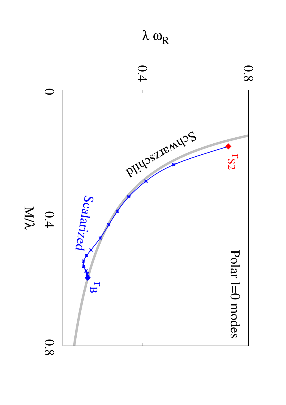
Let us now consider the results for the monopole ( $l=0$ ) modes. They are obtained by starting at the bifurcation point $r_{\rm H}=r_{\rm B}$ , where a corresponding mode of the Schwarzschild solution refers to an independent scalar field in the Schwarzschild background. This mode is given by $M\omega=0.114-i0.090$ . From $r_{\rm B}$ the mode is then tracked along the fundamental branch. The $l=0$ mode is exhibited in Fig. 2, where the scaled eigenvalue $\lambda\omega$ is shown versus the scaled total mass $M/\lambda$ . The left plot exhibits the real part $\omega_{R}$ , representing the frequency, and the right plot exhibits the imaginary part $\omega_{I}$ , representing the inverse damping time. For comparison also the Schwarzschild mode is shown (solid grey). We observe that the scaled frequency of the scalarized black holes of a given mass follows closely the corresponding frequency of the Schwarzschild black holes. The damping rate of the scalarized black holes is always smaller than its Schwarzschild counterpart, thus the damping time is larger for the scalarized solutions.

In Fig. 3 we illustrate the dependence of the scaled eigenvalue $M\omega$ on the scaled scalar charge $Q_{D}/M$ of the black holes. The corresponding Schwarzschild values are read off at $Q_{D}/M=0$ . The scaled frequency varies by less than 20%, whereas the damping rate decreases strongly for larger values of the scaled scalar charge. We emphasize that we do not find unstable modes.

4.2 $l=1$

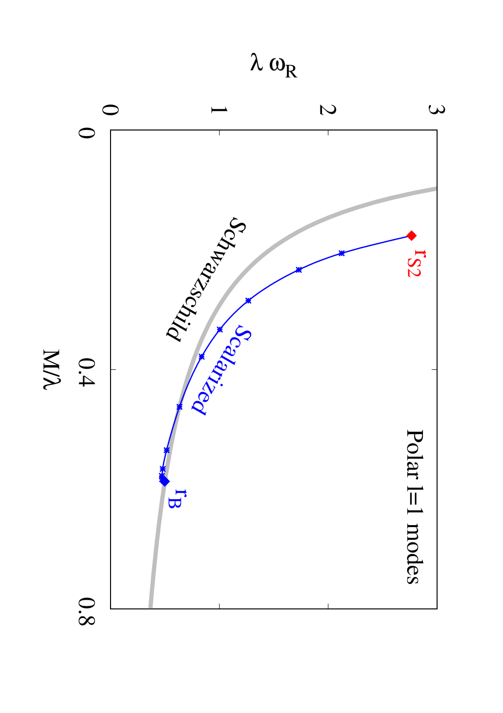
To obtain the dipole ( $l=1$ ) modes, we proceed analogously to the $l=0$ case. We start again at the bifurcation point $r_{\rm H}=r_{\rm B}$ , with the corresponding mode of the Schwarzschild solution $M\omega=0.293-i0.097$ , and then track the mode along the fundamental branch. The $l=1$ mode is exhibited in Fig. 4, where again $\lambda\omega$ is shown versus $M/\lambda$ , with frequency $\omega_{R}$ on the left side and damping rate $\omega_{I}$ on the right. For comparison again the Schwarzschild mode is shown (solid grey). We observe that the frequency and the damping time of the scalarized black holes follow more or less the corresponding frequency and damping time of the Schwarzschild black holes, being mostly slightly larger than their Schwarzschild counterparts. When scaled with the mass and considered as a function of the scalar charge, the deviations from the Schwarzschild values become more pronounced as seen in Fig. 5. Again, we emphasize that we do not find unstable modes.

4.3 $l=2$

In the case of the quadrupole ( $l=2$ ) modes we now have to distinguish between the grav-led modes and the scalar-led modes, since quadrupole modes are also present in the absence of a scalar field. For both families of modes we start again at the bifurcation point $r_{\rm H}=r_{\rm B}$ , where the modes of the Schwarzschild solution are $M\omega=0.3737-i0.08895$ and $M\omega=0.481-i0.0894$ for the gravitational mode and the scalar mode, respectively. Then we track these modes again along the fundamental branch.

The grav-led $l=2$ mode and the scalar-led $l=2$ mode are exhibited in Fig. 6 and Fig. 7, respectively, where again $\lambda\omega$ is shown versus $M/\lambda$ , with frequency $\omega_{R}$ on the left and damping rate $\omega_{I}$ on the right. Again, the Schwarzschild modes are also shown (solid grey). The frequency of the grav-led modes is larger than the frequency of the Schwarzschild modes, with the difference increasing along the branch. The damping rate, in contrast, is smaller than the Schwarzschild damping rate, becoming even very small in some intermediate range, while increasing again towards the Schwarzschild value as the critical point $r_{\rm S2}$ is approached.

The scalar-led mode exhibits less strong deviations from Schwarzschild. The frequency is first slightly smaller than the Schwarzschild value, but then starts to increase more rapidly towards smaller $r_{\rm H}$ . The damping rate, on the other hand, is always larger than the Schwarzschild value. Fig. 8 and Fig. 9 show the frequency and damping time of the grav-led and scalar-led mode again versus the scalar charge. As before, these diagrams enhance the deviations from Schwarzschild. Also for the $l=2$ modes, we emphasize that we do not find unstable modes.

4.4 Isospectrality breaking

The modes of the Schwarzschild black holes are known to exhibit isospectrality, meaning that the polar and the axial mode spectra coincide. Previously it has been observed, that isospectrality is broken in the presence of a dilatonic coupling [24]. This is not surprising, since the scalar field enters the polar equations, while it does not enter the axial equations. Therefore breaking of isospectrality is also expected for EsGB black holes.

We demonstrate the breaking of isospectrality in Fig. 10, where we show the modes $\lambda\omega$ versus $M/\lambda$ (with frequency $\omega_{R}$ on the left and damping rate $\omega_{I}$ on the right), comparing the polar grav-led mode (blue), with the axial mode (red) and also with the isospectral Schwarzschild modes (solid grey). We note, that both the polar grav-led and axial frequencies follow the behavior of the Schwarzschild frequency, but exceed it the more, the smaller the black hole is, with the polar mode frequency increasing faster with decreasing black hole size. The decay rate, on the other hand, follows for the axial case the Schwarzschild decay rate to some extent, whereas the polar case features a completely different decay rate, deviating significantly from the Schwarzschild decay rate except at the boundaries of the relevant range $r_{\rm S2}<r_{\rm H}<r_{\rm B}$ .

5 Conclusions

We have studied the polar quasinormal modes on the fundamental branch of spontaneously scalarized black hole solutions of the EsGB theory proposed and studied in [1]. These scalarized black holes are thermodynamically preferred over the GR ones. However, they should also be dynamically stable or at least sufficiently long-lived to be of astrophysical interest. Here the analysis of their quasinormal modes is an important tool, since it reveals either linear (mode) stability or instability of the black holes, and in case that the black holes are unstable the analysis also provides the time-scale of the instability.

The quasinormal modes consist of polar and axial modes, where the polar modes are composed of radial and non-radial modes. The radial modes were investigated before, where the analysis was focused on the detection of potential instabilities [2]. This analysis revealed the loss of hyperbolicity of the perturbation equations at a critical upper size $r_{\rm S1}$ (for a given coupling constant) for the scalarized black holes. However, for scalarized black holes with sizes in the range between this critical value and the bifurcation point $r_{\rm B}$ from the Schwarzschild branch, no instabilities were detected, making scalarized black holes in this range potentially stable physically interesting objects.

Subsequent investigation of the axial modes of these black holes revealed the loss of hyperbolicity of the perturbation equations at a critical upper size $r_{\rm S2}$ , slightly larger than $r_{\rm S1}$ . Again, no instabilities were detected in the range $r_{\rm S2}<r_{\rm H}<r_{\rm B}$ , retaining a slightly smaller interval of potentially stable physically interesting scalarized black holes [3].

In the present study we have investigated the non-radial polar modes of the black holes in this interval $r_{\rm S2}<r_{\rm H}<r_{\rm B}$ . We have calculated the monopole ( $l=0$ ) modes, the dipole ( $l=1$ ) modes and the quadrupole ( $l=2$ ) modes, where the quadrupole modes consist of grav-led and scalar-led modes. Since we did not find any instabilities, we conclude that the scalarized black holes on the fundamental branch are linearly (mode) stable in the range $r_{\rm S2}<r_{\rm H}<r_{\rm B}$ (for fixed coupling). We note, that we have also continued the analysis of the modes into the range below $r_{\rm S2}$ , where we did not find any further pathologies.

We have compared the frequencies and the damping times of the modes of the scalarized black hole with their Schwarzschild counterparts. We have not seen a general trend for the deviations of the various multipolar modes, which all feature more or less substantial deviations in the frequencies and damping times. An expected outcome of our investigations has been the breaking of isospectrality, i.e., of the degeneracy of the axial and polar Schwarzschild modes. Indeed, in the EsGB black holes we have observed a splitting between the axial modes and the polar grav-led modes as soon as scalarization arises.

This can be relevant with regard to gravitational wave astronomy. With the improvement of sensitivities of the detectors, it could be possible for the LIGO-VIRGO collaboration to measure the ringdown frequencies. In this paper we have quantitatively explored the smoking gun that characterizes the ringdown phase of scalarized black holes in EsGB theory as compared to GR: the richer quasinormal mode spectrum that appears, first, because of the breaking of isospectrality between the grav-led modes in the axial and polar channels, and second, because of the existence of scalar-led modes, that appear at any multipole, and in particular, at $l=0$ . Of course, only stable solutions describing astrophysically conceivable objects are relevant candidates in this respect.

While our study has concluded our linear stability analysis, a non-linear stability analysis would be a natural next objective. On the other hand, investigation of the instabilities of rotating spontaneously scalarized black holes in this theory should also be an interesting and challenging step forward.

Acknowledgements

JLBS, SK, JK and PN gratefully acknowledge support by the DFG funded Research Training Group 1620 “Models of Gravity”. JLBS would like to acknowledge support from the DFG project BL 1553. DD acknowledges financial support via an Emmy Noether Research Group funded by the German Research Foundation (DFG) under grant no. DO 1771/1-1. DD is indebted to the Baden-Württemberg Stiftung for the financial support of this research project by the Eliteprogramme for Postdocs. SY would like to thank the University of Tübingen for the financial support and acknowledges the partial support by the Bulgarian NSF Grant KP-06-H28/7. P.N. is partially supported by the Bulgarian NSF Grant KP-06-H38/2. The authors would also like to acknowledge networking support by the COST Actions CA16104 and CA15117.

Appendix

In this appendix we will present the perturbation equations. Using for the metric the Ansatz (3.1) and for the scalar field the Ansatz (9), we get a system of equations for the polar parity perturbation functions $H_{0},\,H_{1},\,H_{2},\,T$ and $\varphi_{1}$ . For simplicity we introduce the function $K(r)=\frac{1}{1-2m(r)/r}$ . Also in the following equations the prime symbol denotes the derivative with respect to $r$ : $K^{\prime}=\frac{dK}{dr}$ , etc…

We start with the Einstein equations. From the $(t,t)$ -component we get

$\displaystyle{T^{\prime\prime}}$	$\displaystyle=\,{\left(\frac{4\left(K-1\right){\lambda}^{2}}{r\left(-rK{{e}^{{6{\varphi_{0}}}^{2}}}+4\,{\lambda}^{2}{\varphi_{0}^{\prime}}\,{\varphi_{0}}\right)}\right)\varphi_{0}\varphi_{1}^{\prime\prime}}+\,{\left(\frac{-4\,K{\varphi_{0}}\,{\varphi_{0}^{\prime}}\,\left(K-3\right){\lambda}^{2}-2\,{K}^{2}{{e}^{{6{\varphi_{0}}}^{2}}}r{}}{2rK\left(-rK{{e}^{{6{\varphi_{0}}}^{2}}}+4\,{\lambda}^{2}{\varphi_{0}^{\prime}}\,{\varphi_{0}}\right)}\right)H_{2}^{\prime\prime}}$	(20)
$\displaystyle+$	$\displaystyle\,{\left(\frac{\left(-8\,K{\varphi_{0}}\,{\varphi_{0}^{\prime\prime}}\,r+12\,{\varphi_{0}}\,{\varphi_{0}^{\prime}}\,{K^{\prime}}\,r+8\,K{\varphi_{0}^{\prime}}\,\left(12\,{{\varphi_{0}}}^{2}{\varphi_{0}^{\prime}}\,r-{\varphi_{0}^{\prime}}\,r-2\,{\varphi_{0}}\right)\right){\lambda}^{2}}{2rK\left(-rK{{e}^{{6{\varphi_{0}}}^{2}}}+4\,{\lambda}^{2}{\varphi_{0}^{\prime}}\,{\varphi_{0}}\right)}\right.}$
$\displaystyle+$	$\displaystyle{\left.\frac{-K{K^{\prime}}\,{{e}^{{6{\varphi_{0}}}^{2}}}{r}^{2}+6\,{K}^{2}{{e}^{{6{\varphi_{0}}}^{2}}}r}{2rK\left(-rK{{e}^{{6{\varphi_{0}}}^{2}}}+4\,{\lambda}^{2}{\varphi_{0}^{\prime}}\,{\varphi_{0}}\right)}\right)T^{\prime}}$
$\displaystyle+$	$\displaystyle\,{\left(\frac{\left(-4\,{\lambda}^{2}{\varphi_{0}}\,\left(K-3\right){K^{\prime}}-16\,K{\varphi_{0}^{\prime}}\,\left(12\,{{\varphi_{0}}}^{2}-1\right)\left(K-1\right)\right){\lambda}^{2}+4\,{K}^{2}{\varphi_{0}^{\prime}}\,{{e}^{{6{\varphi_{0}}}^{2}}}{r}^{2}}{2rK\left(-rK{{e}^{{6{\varphi_{0}}}^{2}}}+4\,{\lambda}^{2}{\varphi_{0}^{\prime}}\,{\varphi_{0}}\right)}\right)\varphi_{1}^{\prime}}$
$\displaystyle+$	$\displaystyle{\left(\frac{4\,{\lambda}^{2}\left(K-2\right)\varphi_{0}\varphi_{0}^{\prime\prime}}{r\left(rK{{e}^{{6{\varphi_{0}}}^{2}}}-4\,{\lambda}^{2}{\varphi_{0}^{\prime}}\,{\varphi_{0}}\right)}\right.}-{\frac{\left(rK{{e}^{{6{\varphi_{0}}}^{2}}}+2\,K{\lambda}^{2}{\varphi_{0}^{\prime}}\,{\varphi_{0}}-12\,{\lambda}^{2}{\varphi_{0}^{\prime}}\,{\varphi_{0}}\right)K^{\prime}}{rK\left(rK{{e}^{{6{\varphi_{0}}}^{2}}}-4\,{\lambda}^{2}{\varphi_{0}^{\prime}}\,{\varphi_{0}}\right)}}$
$\displaystyle+$	$\displaystyle\,{\frac{2\,K{{\varphi_{0}^{\prime}}}^{2}{{e}^{{6{\varphi_{0}}}^{2}}}{r}^{3}+{K}^{2}{{e}^{{6{\varphi_{0}}}^{2}}}{l}^{2}r+{K}^{2}{{e}^{{6{\varphi_{0}}}^{2}}}lr-96\,K{{\varphi_{0}}}^{2}{{\varphi_{0}^{\prime}}}^{2}{\lambda}^{2}r+2\,rK{{e}^{{6{\varphi_{0}}}^{2}}}-4\,K{\varphi_{0}}\,{\varphi_{0}^{\prime}}\,{l}^{2}{\lambda}^{2}}{2{r}^{2}\left(rK{{e}^{{6{\varphi_{0}}}^{2}}}-4\,{\lambda}^{2}{\varphi_{0}^{\prime}}\,{\varphi_{0}}\right)}}$
$\displaystyle+$	$\displaystyle\left.\frac{192\,{{\varphi_{0}}}^{2}{{\varphi_{0}^{\prime}}}^{2}{\lambda}^{2}r-4\,K{\varphi_{0}}\,{\varphi_{0}^{\prime}}\,l{\lambda}^{2}+8\,K{{\varphi_{0}^{\prime}}}^{2}{\lambda}^{2}r-16\,{{\varphi_{0}^{\prime}}}^{2}{\lambda}^{2}r}{2{r}^{2}\left(rK{{e}^{{6{\varphi_{0}}}^{2}}}-4\,{\lambda}^{2}{\varphi_{0}^{\prime}}\,{\varphi_{0}}\right)}\right)H_{2}$
$\displaystyle+$	$\displaystyle\left(\frac{\left(8\,K{\varphi_{0}}\,\left(K-1\right){\varphi_{0}^{\prime\prime}}-4\,{\varphi_{0}}\,{\varphi_{0}^{\prime}}\,\left(K-3\right){K^{\prime}}-8\,K{{\varphi_{0}^{\prime}}}^{2}\left(12\,{{\varphi_{0}}}^{2}-1\right)\left(K-1\right)\right){\lambda}^{2}}{2rK\left(-rK{{e}^{{6{\varphi_{0}}}^{2}}}+4\,{\lambda}^{2}{\varphi_{0}^{\prime}}\,{\varphi_{0}}\right)}\right.$
$\displaystyle-$	$\displaystyle\left.\frac{2\,K{K^{\prime}}\,{{e}^{{6{\varphi_{0}}}^{2}}}r+2\,{K}^{2}{{e}^{{6{\varphi_{0}}}^{2}}}\left(-{{\varphi_{0}^{\prime}}}^{2}{r}^{2}+K-1\right)}{2rK\left(-rK{{e}^{{6{\varphi_{0}}}^{2}}}+4\,{\lambda}^{2}{\varphi_{0}^{\prime}}\,{\varphi_{0}}\right)}\right)H_{0}$
$\displaystyle+$	$\displaystyle\left(-\,{\frac{2K{\varphi_{0}}\,{\lambda}^{2}\left(l+2\right)\left(l-1\right){\varphi_{0}^{\prime\prime}}}{r\left(rK{{e}^{{6{\varphi_{0}}}^{2}}}-4\,{\lambda}^{2}{\varphi_{0}^{\prime}}\,{\varphi_{0}}\right)}}+{\frac{{\lambda}^{2}{\varphi_{0}^{\prime}}\,{\varphi_{0}}\,\left(l+2\right)\left(l-1\right){K^{\prime}}}{r\left(rK{{e}^{{6{\varphi_{0}}}^{2}}}-4\,{\lambda}^{2}{\varphi_{0}^{\prime}}\,{\varphi_{0}}\right)}}\right)T$
$\displaystyle+$	$\displaystyle\left(\frac{K\left(K{{e}^{{6{\varphi_{0}}}^{2}}}+48\,{{\varphi_{0}}}^{2}{{\varphi_{0}^{\prime}}}^{2}{\lambda}^{2}-4\,{{\varphi_{0}^{\prime}}}^{2}{\lambda}^{2}\right)\left(l+2\right)\left(l-1\right)}{2r\left(rK{{e}^{{6{\varphi_{0}}}^{2}}}-4\,{\lambda}^{2}{\varphi_{0}^{\prime}}\,{\varphi_{0}}\right)}\right)T$
$\displaystyle+$	$\displaystyle\left(\,{\frac{4{\lambda}^{2}\left(12\,{{\varphi_{0}}}^{2}-1\right)\left(K-1\right){\varphi_{0}^{\prime\prime}}}{r\left(rK{{e}^{{6{\varphi_{0}}}^{2}}}-4\,{\lambda}^{2}{\varphi_{0}^{\prime}}\,{\varphi_{0}}\right)}}\right)\varphi_{1}$
$\displaystyle-$	$\displaystyle\,\left({\frac{2{\lambda}^{2}\left(12\,K{{\varphi_{0}}}^{2}{\varphi_{0}^{\prime}}\,r-K{\varphi_{0}}\,l(l+1)-36\,{{\varphi_{0}}}^{2}{\varphi_{0}^{\prime}}\,r-K{\varphi_{0}^{\prime}}\,r+3\,{\varphi_{0}^{\prime}}\,r\right){K^{\prime}}}{K{r}^{2}\left(rK{{e}^{{6{\varphi_{0}}}^{2}}}-4\,{\lambda}^{2}{\varphi_{0}^{\prime}}\,{\varphi_{0}}\right)}}\right)\varphi_{1}$
$\displaystyle-$	$\displaystyle\left(\,{\frac{144{\varphi_{0}}\,{{\varphi_{0}^{\prime}}}^{2}{\lambda}^{2}\left(2\,{\varphi_{0}}-1\right)\left(2\,{\varphi_{0}}+1\right)\left(K-1\right)}{r\left(rK{{e}^{6{{\varphi_{0}}}^{2}}}-4\,{\lambda}^{2}{\varphi_{0}^{\prime}}\,{\varphi_{0}}\right)}}\right){\varphi_{1}}$

From the $(t,r)$ -component we get

$\displaystyle{T^{\prime}}$	$\displaystyle=\,{\left(\frac{4\,\left(K-1\right){\lambda}^{2}}{r\left(-rK{{e}^{{6{\varphi_{0}}}^{2}}}+4\,{\lambda}^{2}{\varphi_{0}^{\prime}}\,{\varphi_{0}}\right)}\right)\varphi_{0}\varphi_{1}^{\prime}}+\,{\left(\frac{-4\,f{\varphi_{0}}\,{\varphi_{0}^{\prime}}\,\left(K-3\right){\lambda}^{2}-2\,{{e}^{{6{\varphi_{0}}}^{2}}}fKr}{2rf\left(-rK{{e}^{{6{\varphi_{0}}}^{2}}}+4\,{\lambda}^{2}{\varphi_{0}^{\prime}}\,{\varphi_{0}}\right)}\right)H_{2}}$	(21)
$\displaystyle+$	$\displaystyle\,\left({\frac{2\,{{e}^{{6{\varphi_{0}}}^{2}}}K{{\varphi_{0}^{\prime}}}^{2}{r}^{3}+{{e}^{{6{\varphi_{0}}}^{2}}}{K}^{2}(l+2)(l-1))r-2\,{{e}^{{6{\varphi_{0}}}^{2}}}{K}^{2}r+2\,rK{{e}^{{6{\varphi_{0}}}^{2}}}-96K{{\varphi_{0}}}^{2}{{\varphi_{0}^{\prime}}}^{2}{\lambda}^{2}r}{2K{r}^{2}\left(rK{{e}^{{6{\varphi_{0}}}^{2}}}-4\,{\lambda}^{2}{\varphi_{0}^{\prime}}\,{\varphi_{0}}\right)}}\right.$
$\displaystyle+$	$\displaystyle\,{\frac{96\,{{\varphi_{0}}}^{2}{{\varphi_{0}^{\prime}}}^{2}{\lambda}^{2}r+8\,{\varphi_{0}^{\prime\prime}}\,(K-1){\varphi_{0}}\,{\lambda}^{2}r-4\,K{\varphi_{0}}\,{\varphi_{0}^{\prime}}\,{\lambda}^{2}l(l+1)-8\,{{\varphi_{0}^{\prime}}}^{2}{\lambda}^{2}r(1-K)}{2K{r}^{2}\left(rK{{e}^{{6{\varphi_{0}}}^{2}}}-4\,{\lambda}^{2}{\varphi_{0}^{\prime}}\,{\varphi_{0}}\right)}}$
$\displaystyle-$	$\displaystyle\left.{\frac{\left(rK{{e}^{{6{\varphi_{0}}}^{2}}}+2\,K{\lambda}^{2}{\varphi_{0}^{\prime}}\,{\varphi_{0}}-6\,{\lambda}^{2}{\varphi_{0}^{\prime}}\,{\varphi_{0}}\right){K^{\prime}}}{r\left(rK{{e}^{{6{\varphi_{0}}}^{2}}}-4\,{\lambda}^{2}{\varphi_{0}^{\prime}}\,{\varphi_{0}}\right){K}^{2}}}\right)\frac{H_{1}}{\omega}$
$\displaystyle+$	$\displaystyle\,{\left(\frac{-4\,\left(K-1\right)\left(24\,f{{\varphi_{0}}}^{2}{\varphi_{0}^{\prime}}+{f^{\prime}}\,{\varphi_{0}}-2\,f{\varphi_{0}^{\prime}}\right){\lambda}^{2}+4\,{{e}^{{6{\varphi_{0}}}^{2}}}fK{\varphi_{0}^{\prime}}\,{r}^{2}}{2rf\left(-rK{{e}^{{6{\varphi_{0}}}^{2}}}+4\,{\lambda}^{2}{\varphi_{0}^{\prime}}\,{\varphi_{0}}\right)}\right)\varphi_{1}}$
$\displaystyle+$	$\displaystyle{\left(\frac{4\,{\varphi_{0}}\,{\varphi_{0}^{\prime}}\,\left({f^{\prime}}\,r-2\,f\right){\lambda}^{2}-rK{{e}^{{6{\varphi_{0}}}^{2}}}\left({f^{\prime}}\,r-2\,f\right)}{2rf\left(-rK{{e}^{{6{\varphi_{0}}}^{2}}}+4\,{\lambda}^{2}{\varphi_{0}^{\prime}}\,{\varphi_{0}}\right)}\right)T}\,.$

From the $(t,\varphi)$ -component we get

$\displaystyle{H_{1}^{\prime}}$	$\displaystyle=$	$\displaystyle K\omega H_{2}-{\frac{4{\lambda}^{2}{\varphi_{0}}{K^{\prime}}}{4{\lambda}^{2}{\varphi_{0}}{\varphi_{0}^{\prime}}-rK{{e}^{6{{\varphi_{0}}}^{2}}}}}\omega\varphi_{1}-{\frac{-{f^{\prime}}{{e}^{6{{\varphi_{0}}}^{2}}}{K}^{2}{r}^{2}+{K^{\prime}}{{e}^{6{{\varphi_{0}}}^{2}}}f{r}^{2}K}{2fKr\left(4{\lambda}^{2}{\varphi_{0}}{\varphi_{0}^{\prime}}-rK{{e}^{6{{\varphi_{0}}}^{2}}}\right)}}{H_{1}}$	(22)
	$\displaystyle-$	$\displaystyle{\frac{\left(2{\varphi_{0}}{\varphi_{0}^{\prime}}{K^{\prime}}r-4K{\varphi_{0}}{\varphi_{0}^{\prime\prime}}r+4K{{\varphi_{0}^{\prime}}}^{2}r\left(12{{\varphi_{0}}}^{2}-1\right)\right){\lambda}^{2}+{K}^{2}{{e}^{6{{\varphi_{0}}}^{2}}}r}{4{\lambda}^{2}{\varphi_{0}}{\varphi_{0}^{\prime}}-rK{{e}^{6{{\varphi_{0}}}^{2}}}}}\omega T$
	$\displaystyle-$	$\displaystyle{\frac{4fK{\varphi_{0}}{\varphi_{0}^{\prime\prime}}r-6f{\varphi_{0}}{\varphi_{0}^{\prime}}{K^{\prime}}r+2K{\varphi_{0}^{\prime}}\left(2f{\varphi_{0}^{\prime}}r(1-12{{\varphi_{0}}}^{2})+{\varphi_{0}}({f^{\prime}}r-2f)\right)}{fKr\left(4{\lambda}^{2}{\varphi_{0}}{\varphi_{0}^{\prime}}-rK{{e}^{6{{\varphi_{0}}}^{2}}}\right)}}{\lambda}^{2}{H_{1}}\,.$

From the $(r,r)$ -component we get

$\displaystyle{H_{0}^{\prime}}$	$\displaystyle=\left({\frac{\left(12\,{\varphi_{0}}\,{\varphi_{0}^{\prime}}\,{\lambda}^{2}{r}-{{e}^{6\,{{\varphi_{0}}}^{2}}}K{r}^{2}\right){f^{\prime}}}{2f\left(2\,{\varphi_{0}}\,{\varphi_{0}^{\prime}}\,\left(K-3\right){\lambda}^{2}+rK{{e}^{6\,{{\varphi_{0}}}^{2}}}\right)}}-{\frac{rK{{e}^{6\,{{\varphi_{0}}}^{2}}}}{2\,{\varphi_{0}}\,{\varphi_{0}^{\prime}}\,\left(K-3\right){\lambda}^{2}+rK{{e}^{6\,{{\varphi_{0}}}^{2}}}}}\right){T^{\prime}}$	(23)
$\displaystyle+$	$\displaystyle\left(\,{\frac{-2{\varphi_{0}}\,\left(K-3\right){\lambda}^{2}{f^{\prime}}}{f\left(2\,{\varphi_{0}}\,{\varphi_{0}^{\prime}}\,\left(K-3\right){\lambda}^{2}+rK{{e}^{6\,{{\varphi_{0}}}^{2}}}\right)}}+\,{\frac{2{{e}^{6\,{{\varphi_{0}}}^{2}}}K{\varphi_{0}^{\prime}}\,{r}^{2}}{2\,{\varphi_{0}}\,{\varphi_{0}^{\prime}}\,\left(K-3\right){\lambda}^{2}+rK{{e}^{6\,{{\varphi_{0}}}^{2}}}}}\right){\varphi_{1}^{\prime}}$
$\displaystyle+$	$\displaystyle\left(\,{\frac{-6{\lambda}^{2}{f^{\prime}}\,{\varphi_{0}^{\prime}}\,{\varphi_{0}}}{f\left(2\,{\varphi_{0}}\,{\varphi_{0}^{\prime}}\,\left(K-3\right){\lambda}^{2}+rK{{e}^{6\,{{\varphi_{0}}}^{2}}}\right)}}+{\frac{{{e}^{6\,{{\varphi_{0}}}^{2}}}{K}^{2}}{2\,{\varphi_{0}}\,{\varphi_{0}^{\prime}}\,\left(K-3\right){\lambda}^{2}+rK{{e}^{6\,{{\varphi_{0}}}^{2}}}}}\right){H_{2}}$
$\displaystyle+$	$\displaystyle\,{\left(\frac{8\,{\varphi_{0}}\,{\varphi_{0}^{\prime}}\,r\left(K-3\right){\lambda}^{2}+4\,{{e}^{6\,{{\varphi_{0}}}^{2}}}K{r}^{2}}{2rf\left(2\,{\varphi_{0}}\,{\varphi_{0}^{\prime}}\,\left(K-3\right){\lambda}^{2}+rK{{e}^{6\,{{\varphi_{0}}}^{2}}}\right)}\right)\omega H_{1}}$
$\displaystyle+$	$\displaystyle\,{\left(\frac{-4\,fK{\varphi_{0}}\,{\varphi_{0}^{\prime}}\,l\left(l+1\right){\lambda}^{2}+{{e}^{6\,{{\varphi_{0}}}^{2}}}f{K}^{2}lr\left(l+1\right)}{2rf\left(2\,{\varphi_{0}}\,{\varphi_{0}^{\prime}}\,\left(K-3\right){\lambda}^{2}+rK{{e}^{6\,{{\varphi_{0}}}^{2}}}\right)}\right)H_{0}}$
$\displaystyle+$	$\displaystyle\left(-{\frac{K{\varphi_{0}}\,{\varphi_{0}^{\prime}}\,\left(l+2\right)\left(l-1\right){\lambda}^{2}{f^{\prime}}}{f\left(2\,{\varphi_{0}}\,{\varphi_{0}^{\prime}}\,\left(K-3\right){\lambda}^{2}+rK{{e}^{6\,{{\varphi_{0}}}^{2}}}\right)}}+\,{\frac{\left(8\,K{\varphi_{0}}\,{\varphi_{0}^{\prime}}\,{\lambda}^{2}{r}^{2}-2\,{{e}^{6\,{{\varphi_{0}}}^{2}}}{K}^{2}{r}^{3}\right){\omega}^{2}}{2rf\left(2\,{\varphi_{0}}\,{\varphi_{0}^{\prime}}\,\left(K-3\right){\lambda}^{2}+rK{{e}^{6\,{{\varphi_{0}}}^{2}}}\right)}}\right.$
$\displaystyle+$	$\displaystyle\,\left.{\frac{{{e}^{6\,{{\varphi_{0}}}^{2}}}{K}^{2}\left(l+2\right)\left(l-1\right)}{4\,{\varphi_{0}}\,{\varphi_{0}^{\prime}}\,\left(K-3\right){\lambda}^{2}+2rK{{e}^{6\,{{\varphi_{0}}}^{2}}}}}\right)T$
$\displaystyle+$	$\displaystyle\left(\,{\frac{\left(48\,K{{\varphi_{0}}}^{2}{\varphi_{0}^{\prime}}\,r-4\,K{\varphi_{0}}\,{l}^{2}-144\,{{\varphi_{0}}}^{2}{\varphi_{0}^{\prime}}\,r-4\,K{\varphi_{0}^{\prime}}\,r-4\,K{\varphi_{0}}\,l+12\,{\varphi_{0}^{\prime}}\,r\right){\lambda}^{2}{f^{\prime}}}{2rf\left(2\,{\varphi_{0}}\,{\varphi_{0}^{\prime}}\,\left(K-3\right){\lambda}^{2}+rK{{e}^{6\,{{\varphi_{0}}}^{2}}}\right)}}\right.$
$\displaystyle-$	$\displaystyle\left.\,{\frac{4K{\varphi_{0}}\,\left(K-1\right){\lambda}^{2}{\omega}^{2}}{f\left(2\,{\varphi_{0}}\,{\varphi_{0}^{\prime}}\,\left(K-3\right){\lambda}^{2}+rK{{e}^{6\,{{\varphi_{0}}}^{2}}}\right)}}\right){\varphi_{1}}\,.$

From the $(r,\theta)$ -component we get

$\displaystyle{T^{\prime}}$	$\displaystyle={\left(\frac{2\,{{e}^{{6{\varphi_{0}}}^{2}}}fK{r}^{2}-8\,f{\varphi_{0}}\,{\varphi_{0}^{\prime}}\,{\lambda}^{2}r}{2{r}^{2}\left(-K{{e}^{{6{\varphi_{0}}}^{2}}}f+2\,{\lambda}^{2}{f^{\prime}}\,{\varphi_{0}^{\prime}}\,{\varphi_{0}}\right)}\right)H_{0}^{\prime}}-{\left(\frac{4{f^{\prime}}\,{\lambda}^{2}}{r\left(-K{{e}^{{6{\varphi_{0}}}^{2}}}f+2\,{\lambda}^{2}{f^{\prime}}\,{\varphi_{0}^{\prime}}\,{\varphi_{0}}\right)}\right)\varphi_{0}\varphi_{1}^{\prime}}$	(24)
$\displaystyle+$	$\displaystyle{\left(\frac{12\,{f^{\prime}}\,{\varphi_{0}}\,{\varphi_{0}^{\prime}}\,{\lambda}^{2}r-{{e}^{{6{\varphi_{0}}}^{2}}}Kr\left({f^{\prime}}\,r+2\,f\right)}{2{r}^{2}\left(-K{{e}^{{6{\varphi_{0}}}^{2}}}f+2\,{\lambda}^{2}{f^{\prime}}\,{\varphi_{0}^{\prime}}\,{\varphi_{0}}\right)}\right)H_{2}}+{\left(\frac{-2\,\left({{e}^{{{\varphi_{0}}}^{2}}}\right)^{6}K{r}^{2}+8\,{\varphi_{0}}\,{\varphi_{0}^{\prime}}\,{\lambda}^{2}r}{2{r}^{2}\left(-K\left({{e}^{{{\varphi_{0}}}^{2}}}\right)^{6}f+2\,{\lambda}^{2}{f^{\prime}}\,{\varphi_{0}^{\prime}}\,{\varphi_{0}}\right)}\right)\omega H_{1}}$
$\displaystyle+$	$\displaystyle{\left(\frac{-4\,{\varphi_{0}}\,{\varphi_{0}^{\prime}}\,\left({f^{\prime}}\,r-2\,f\right){\lambda}^{2}+rK\left({{e}^{{{\varphi_{0}}}^{2}}}\right)^{6}\left({f^{\prime}}\,r-2\,f\right)}{2{r}^{2}\left(-K{{e}^{{6{\varphi_{0}}}^{2}}}f+2\,{\lambda}^{2}{f^{\prime}}\,{\varphi_{0}^{\prime}}\,{\varphi_{0}}\right)}\right)H_{0}}$
$\displaystyle+$	$\displaystyle{\left(\frac{8\,{f^{\prime}}\,\left(12\,{{\varphi_{0}}}^{2}{\varphi_{0}^{\prime}}\,r-{\varphi_{0}^{\prime}}\,r+{\varphi_{0}}\right){\lambda}^{2}+8\,{{e}^{{6{\varphi_{0}}}^{2}}}fK{\varphi_{0}^{\prime}}\,{r}^{2}}{2{r}^{2}\left(-K{{e}^{{6{\varphi_{0}}}^{2}}}f+2\,{\lambda}^{2}{f^{\prime}}\,{\varphi_{0}^{\prime}}\,{\varphi_{0}}\right)}\right)\varphi_{1}}\,.$

From the $(\theta,\phi)$ -component we get

		$\displaystyle{H_{2}}$	$\displaystyle={\left(\frac{f\left(\left(-4\,K{\varphi_{0}}\,{\varphi_{0}^{\prime\prime}}+2\,{\varphi_{0}}\,{K^{\prime}}\,{\varphi_{0}^{\prime}}+4\,K{{\varphi_{0}^{\prime}}}^{2}\left(12\,{{\varphi_{0}}}^{2}-1\right)\right){\lambda}^{2}+{K}^{2}{{e}^{6{{\varphi_{0}}}^{2}}}\right)}{\left(-K{{e}^{{6{\varphi_{0}}}^{2}}}f+2\,{\lambda}^{2}{f^{\prime}}\,{\varphi_{0}^{\prime}}\,{\varphi_{0}}\right)K}\right)H_{0}}$		(25)
		$\displaystyle+$	$\displaystyle\,{\left(\frac{2{\lambda}^{2}\left({f^{\prime}}\,f{K^{\prime}}-K\left(2\,f{f^{\prime\prime}}-{{f^{\prime}}}^{2}\right)\right)}{\left(-K{{e}^{{6{\varphi_{0}}}^{2}}}f+2\,{\lambda}^{2}{f^{\prime}}\,{\varphi_{0}^{\prime}}\,{\varphi_{0}}\right)fK}\right)\varphi_{0}\varphi_{1}}\,.$		(25)

Finally, from the scalar field equation we get

$\displaystyle\varphi_{1}^{\prime\prime}$	$\displaystyle=\left(-{\frac{{f^{\prime}}{\varphi_{0}}\left(K-3\right){\lambda}^{2}}{2fK{r}^{2}\left({{e}^{6{{\varphi_{0}}}^{2}}}\right)}}+\frac{\varphi_{0}^{\prime}}{2}\right){H_{2}^{\prime}}+{\left(\frac{{\varphi_{0}}f\left(K-1\right){\lambda}^{2}}{fK{r}^{2}\left({{e}^{{6{\varphi_{0}}}^{2}}}\right)}\right)}{H_{0}^{\prime\prime}}-{\left(\frac{{\varphi_{0}}{f^{\prime}}r{\lambda}^{2}}{fK{r}^{2}\left({{e}^{{6{\varphi_{0}}}^{2}}}\right)}\right)}{T^{\prime\prime}}$	(26)
$\displaystyle+$	$\displaystyle\left({\frac{{K^{\prime}}}{2K}}-{\frac{{f^{\prime}}r+4f}{2fr}}\right){\varphi_{1}^{\prime}}+\left({\frac{Kl\left(l+1\right)}{{r}^{2}}}-{\frac{K{\omega}^{2}}{f}}\right)\varphi_{1}$
$\displaystyle-$	$\displaystyle{\left(\frac{2{\varphi_{0}}\left(K-1\right){\lambda}^{2}\omega}{fK{r}^{2}\left({{e}^{{6{\varphi_{0}}}^{2}}}\right)}\right)}{H_{1}^{\prime}}+\left(\left(-{\frac{{\varphi_{0}}\left(K-3\right){K^{\prime}}}{2{r}^{2}\left({{e}^{{6{\varphi_{0}}}^{2}}}\right){K}^{2}}}+{\frac{{f^{\prime}}{\varphi_{0}}\left(K-1\right)}{fK{r}^{2}\left({{\rm e}^{{{\varphi_{0}}}^{2}}}\right)^{6}}}\right){\lambda}^{2}-\frac{\varphi_{0}^{\prime}}{2}\right){H_{0}^{\prime}}$
$\displaystyle+$	$\displaystyle\left(\left({\frac{3{f^{\prime}}{\varphi_{0}}{K^{\prime}}}{2fr\left({{e}^{{6{\varphi_{0}}}^{2}}}\right){K}^{2}}}+{\frac{{\varphi_{0}}\left(-2{f^{\prime\prime}}fr+{{f^{\prime}}}^{2}r-4{f^{\prime}}f\right)}{2K{r}^{2}{f}^{2}\left({{e}^{{6{\varphi_{0}}}^{2}}}\right)}}\right){\lambda}^{2}-{\varphi_{0}^{\prime}}\right){T^{\prime}}$
$\displaystyle+$	$\displaystyle\left({\frac{{\varphi_{0}}\left(K-1\right){\lambda}^{2}{\omega}^{2}}{f{r}^{2}\left({{e}^{{6{\varphi_{0}}}^{2}}}\right)}}+{\varphi_{0}^{\prime\prime}}-{\frac{{\varphi_{0}^{\prime}}{K^{\prime}}}{2K}}+{\frac{{\varphi_{0}^{\prime}}\left({f^{\prime}}r+4f\right)}{2fr}}\right){H_{2}}$
$\displaystyle+$	$\displaystyle\left(\left({\frac{{f^{\prime}}{\varphi_{0}}\left(K-6\right){K^{\prime}}}{2f{r}^{2}\left({{e}^{{6{\varphi_{0}}}^{2}}}\right){K}^{2}}}+{\frac{{\varphi_{0}}\left({f^{\prime}}{l(l+1)}fK+(2{f^{\prime\prime}}fr-{{f^{\prime}}}^{2}r)(2-K)\right)}{2K{f}^{2}\left({{e}^{{6{\varphi_{0}}}^{2}}}\right){r}^{3}}}\right){\lambda}^{2}\right){H_{2}}$
$\displaystyle+$	$\displaystyle\left({\frac{{\varphi_{0}}\left(K-3\right){K^{\prime}}{\lambda}^{2}}{f{r}^{2}\left({{e}^{{6{\varphi_{0}}}^{2}}}\right){K}^{2}}}+{\frac{{\varphi_{0}^{\prime}}}{f}}\right)\omega H_{1}-{\left(\frac{{\varphi_{0}}l\left(l+1\right){K^{\prime}}{\lambda}^{2}}{2\left({{e}^{{6{\varphi_{0}}}^{2}}}\right)K{r}^{3}}\right)}H_{0}$
$\displaystyle+$	$\displaystyle\left({\frac{{K^{\prime}}{\varphi_{0}}{\lambda}^{2}{\omega}^{2}}{rKf\left({{e}^{{6{\varphi_{0}}}^{2}}}\right)}}+\left({\frac{{f^{\prime}}{\varphi_{0}}\left(l+2\right)\left(1-l\right){K^{\prime}}}{4fK{r}^{2}\left({{e}^{6{{\varphi_{0}}}^{2}}}\right)}}-{\frac{{\varphi_{0}}\left({{f^{\prime}}}^{2}-2{f^{\prime\prime}}f\right)\left(l+2\right)\left(l-1\right)}{4{r}^{2}{f}^{2}\left({{e}^{{6{\varphi_{0}}}^{2}}}\right)}}\right){\lambda}^{2}\right)T$
$\displaystyle+$	$\displaystyle\left(\left({\frac{{f^{\prime}}\left(12{{\varphi_{0}}}^{2}-1\right)\left(K-3\right){K^{\prime}}}{2f{r}^{2}\left({{e}^{{6{\varphi_{0}}}^{2}}}\right){K}^{2}}}+{\frac{\left(12{{\varphi_{0}}}^{2}-1\right)\left(K-1\right)\left({{f^{\prime}}}^{2}-2{f^{\prime\prime}}f\right)}{2K{r}^{2}{f}^{2}\left({{e}^{{6{\varphi_{0}}}^{2}}}\right)}}\right){\lambda}^{2}\right)\varphi_{1}\,.$

The remaining components of the Einstein equations are zero or can be written in terms of the previous components.

This system of equations can be further simplified. After some algebra we can derive an equation which relates the function $H_{0}$ to the rest of the metric perturbation functions, as well as the perturbation of the scalar field $\varphi_{1}$ and its derivative. Using this relation and the algebraic relation $(\ref{pert_tphi})$ we can eliminate the functions $H_{0}$ and $H_{2}$ , and reduce the perturbation equations to a coupled system of three differential equations for the remaining metric perturbation functions $H_{1}$ and $T$ and the perturbation of the scalar field $\varphi_{1}$ . It can be proven that these equations together with the two relations representing the functions $H_{0}$ and $H_{2}$ in terms of the rest of the perturbation functions are equivalent to the initial set of perturbation equations.

The system of equations for the perturbations functions $H_{1}$ , $T$ and $\varphi_{1}$ can be represented schematically in the form

\left(\begin{array}[]{c}H_{1}^{\prime}\\ T^{\prime}\\ \varphi_{1}^{\prime}\\ \varphi_{1}^{\prime\prime}\end{array}\right)+\left(\begin{array}[]{c}V_{11}\;\;V_{12}\;\;V_{13}\;\;V_{14}\\ V_{21}\;\;V_{22}\;\;V_{23}\;\;V_{24}\\ V_{31}\;\;V_{32}\;\;V_{33}\;\;V_{34}\\ V_{41}\;\;V_{42}\;\;V_{43}\;\;V_{44}\end{array}\right)\left(\begin{array}[]{c}H_{1}\\ T\\ \varphi_{1}\\ \varphi_{1}^{\prime}\end{array}\right)=0,

(27)

where $V_{3k}=0$ for $k\neq 4$ , and $V_{34}=-1$ . Due to the complexity of the components of $V_{p}$ , we shall not show them here. However, by making the dependence in $\omega$ explicit, we can write the previous equation like

\left(\begin{array}[]{c}H_{1}^{\prime}/\omega\\ T^{\prime}\\ \varphi_{1}^{\prime}\\ \varphi_{1}^{\prime\prime}\end{array}\right)+\left[\left(\begin{array}[]{c}V_{11}^{(1)}\;\;V_{12}^{(1)}\;\;V_{13}^{(1)}\;\;V_{14}^{(1)}\\ V_{21}^{(1)}\;\;V_{22}^{(1)}\;\;V_{23}^{(1)}\;\;V_{24}^{(1)}\\ 0\;\;\;\;\;\;0\;\;\;\;\;\;0\;\;\;\;\;\;-1\\ V_{41}^{(1)}\;\;V_{42}^{(1)}\;\;V_{43}^{(1)}\;\;V_{44}^{(1)}\end{array}\right)+\omega^{2}\left(\begin{array}[]{c}V_{11}^{(2)}\;\;V_{12}^{(2)}\;\;V_{13}^{(2)}\;\;\;0\\ V_{21}^{(2)}\;\;V_{22}^{(2)}\;\;V_{23}^{(2)}\;\;\;0\\ 0\;\;\;\;\;\;\;0\;\;\;\;\;\;\;0\;\;\;\;\;\;\;0\\ V_{41}^{(2)}\;\;V_{42}^{(2)}\;\;V_{43}^{(2)}\;\;\;0\end{array}\right)\right]\left(\begin{array}[]{c}H_{1}/\omega\\ T\\ \varphi_{1}\\ \varphi_{1}^{\prime}\end{array}\right)=0,

(28)

where the functions $V_{ij}^{(1,2)}$ only depend on $f(r)$ , $m(r)$ , $\varphi_{0}(r)$ , $\lambda$ and $l$ .

The boundary conditions for the perturbations can be found with the help of the expansions of the background metric and the scalar field. Because of the natural divergence at spatial infinity, one has to consider a high-order expansion of the perturbations at infinity for the quasinormal modes.

For the lowest values $l=0,1$ , simpler gauge choices can be chosen [49]. We note that for $l=1$ we can choose a gauge in which $T$ vanishes identically. Therefore, we can use the first two equations in (28) to eliminate $H_{1}^{\prime}$ and $H_{1}$ in favor of $\varphi_{1}$ , $\varphi_{1}^{\prime}$ . In the case of $l=0$ we can pick a gauge such that both $T$ and $H_{1}$ vanish. The equations are then again reduced to a second order equation for the scalar perturbation. This is possible since some harmonics in the expansion are identically zero when $l=0$ or $l=1$ .

References

[1] D. D. Doneva and S. S. Yazadjiev, “New Gauss-Bonnet Black Holes with Curvature-Induced Scalarization in Extended Scalar-Tensor Theories,” Phys. Rev. Lett., vol. 120, no. 13, p. 131103, 2018.
[2] J. L. Blazquez-Salcedo, D. D. Doneva, J. Kunz, and S. S. Yazadjiev, “Radial perturbations of the scalarized Einstein-Gauss-Bonnet black holes,” Phys. Rev., vol. D98, no. 8, p. 084011, 2018.
[3] J. L. Blazquez-Salcedo, D. D. Doneva, S. Kahlen, J. Kunz, P. Nedkova, and S. S. Yazadjiev, “Axial perturbations of the scalarized Einstein-Gauss-Bonnet black holes,” Phys. Rev. D, vol. 101, no. 10, p. 104006, 2020.
[4] B. P. Abbott et al., “Tests of general relativity with GW150914,” Phys. Rev. Lett., vol. 116, no. 22, p. 221101, 2016. [Erratum: Phys. Rev. Lett.121,no.12,129902(2018)].
[5] B. P. Abbott et al., “Tests of General Relativity with GW170817,” Phys. Rev. Lett., vol. 123, no. 1, p. 011102, 2019.
[6] B. P. Abbott et al., “Tests of General Relativity with the Binary Black Hole Signals from the LIGO-Virgo Catalog GWTC-1,” Phys. Rev., vol. D100, no. 10, p. 104036, 2019.
[7] C. M. Will, “The Confrontation between General Relativity and Experiment,” Living Rev. Rel., vol. 17, p. 4, 2014.
[8] E. Berti et al., “Testing General Relativity with Present and Future Astrophysical Observations,” Class. Quant. Grav., vol. 32, p. 243001, 2015.
[9] L. Barack et al., “Black holes, gravitational waves and fundamental physics: a roadmap,” Class. Quant. Grav., vol. 36, no. 14, p. 143001, 2019.
[10] G. W. Horndeski, “Second-order scalar-tensor field equations in a four-dimensional space,” Int. J. Theor. Phys., vol. 10, pp. 363–384, 1974.
[11] C. Charmousis, E. J. Copeland, A. Padilla, and P. M. Saffin, “General second order scalar-tensor theory, self tuning, and the Fab Four,” Phys. Rev. Lett., vol. 108, p. 051101, 2012.
[12] T. Kobayashi, M. Yamaguchi, and J. Yokoyama, “Generalized G-inflation: Inflation with the most general second-order field equations,” Prog. Theor. Phys., vol. 126, pp. 511–529, 2011.
[13] P. Kanti, N. Mavromatos, J. Rizos, K. Tamvakis, and E. Winstanley, “Dilatonic black holes in higher curvature string gravity,” Phys. Rev. D, vol. 54, pp. 5049–5058, 1996.
[14] T. Torii, H. Yajima, and K.-i. Maeda, “Dilatonic black holes with Gauss-Bonnet term,” Phys. Rev. D, vol. 55, pp. 739–753, 1997.
[15] Z.-K. Guo, N. Ohta, and T. Torii, “Black Holes in the Dilatonic Einstein-Gauss-Bonnet Theory in Various Dimensions. I. Asymptotically Flat Black Holes,” Prog. Theor. Phys., vol. 120, pp. 581–607, 2008.
[16] P. Pani and V. Cardoso, “Are black holes in alternative theories serious astrophysical candidates? The Case for Einstein-Dilaton-Gauss-Bonnet black holes,” Phys. Rev., vol. D79, p. 084031, 2009.
[17] P. Pani, C. F. Macedo, L. C. Crispino, and V. Cardoso, “Slowly rotating black holes in alternative theories of gravity,” Phys. Rev. D, vol. 84, p. 087501, 2011.
[18] B. Kleihaus, J. Kunz, and E. Radu, “Rotating Black Holes in Dilatonic Einstein-Gauss-Bonnet Theory,” Phys. Rev. Lett., vol. 106, p. 151104, 2011.
[19] D. Ayzenberg, K. Yagi, and N. Yunes, “Linear Stability Analysis of Dynamical Quadratic Gravity,” Phys. Rev. D, vol. 89, no. 4, p. 044023, 2014.
[20] D. Ayzenberg and N. Yunes, “Slowly-Rotating Black Holes in Einstein-Dilaton-Gauss-Bonnet Gravity: Quadratic Order in Spin Solutions,” Phys. Rev. D, vol. 90, p. 044066, 2014. [Erratum: Phys.Rev.D 91, 069905 (2015)].
[21] A. Maselli, P. Pani, L. Gualtieri, and V. Ferrari, “Rotating black holes in Einstein-Dilaton-Gauss-Bonnet gravity with finite coupling,” Phys. Rev. D, vol. 92, no. 8, p. 083014, 2015.
[22] B. Kleihaus, J. Kunz, and S. Mojica, “Quadrupole Moments of Rapidly Rotating Compact Objects in Dilatonic Einstein-Gauss-Bonnet Theory,” Phys. Rev. D, vol. 90, no. 6, p. 061501, 2014.
[23] B. Kleihaus, J. Kunz, S. Mojica, and E. Radu, “Spinning black holes in Einstein–Gauss-Bonnet–dilaton theory: Nonperturbative solutions,” Phys. Rev. D, vol. 93, no. 4, p. 044047, 2016.
[24] J. L. Blazquez-Salcedo, C. F. B. Macedo, V. Cardoso, V. Ferrari, L. Gualtieri, F. S. Khoo, J. Kunz, and P. Pani, “Perturbed black holes in Einstein-dilaton-Gauss-Bonnet gravity: Stability, ringdown, and gravitational-wave emission,” Phys. Rev., vol. D94, no. 10, p. 104024, 2016.
[25] P. V. Cunha, C. A. R. Herdeiro, B. Kleihaus, J. Kunz, and E. Radu, “Shadows of Einstein–dilaton–Gauss–Bonnet black holes,” Phys. Lett. B, vol. 768, pp. 373–379, 2017.
[26] H. Zhang, M. Zhou, C. Bambi, B. Kleihaus, J. Kunz, and E. Radu, “Testing Einstein-dilaton-Gauss-Bonnet gravity with the reflection spectrum of accreting black holes,” Phys. Rev. D, vol. 95, no. 10, p. 104043, 2017.
[27] J. L. Blazquez-Salcedo, F. S. Khoo, and J. Kunz, “Quasinormal modes of Einstein-Gauss-Bonnet-dilaton black holes,” Phys. Rev., vol. D96, no. 6, p. 064008, 2017.
[28] R. A. Konoplya, A. F. Zinhailo, and Z. Stuchlík, “Quasinormal modes, scattering, and Hawking radiation in the vicinity of an Einstein-dilaton-Gauss-Bonnet black hole,” Phys. Rev., vol. D99, no. 12, p. 124042, 2019.
[29] A. F. Zinhailo, “Quasinormal modes of Dirac field in the Einstein–Dilaton–Gauss–Bonnet and Einstein–Weyl gravities,” Eur. Phys. J., vol. C79, no. 11, p. 912, 2019.
[30] P. T. Chrusciel, J. Lopes Costa, and M. Heusler, “Stationary Black Holes: Uniqueness and Beyond,” Living Rev. Rel., vol. 15, p. 7, 2012.
[31] C. A. Herdeiro and E. Radu, “Asymptotically flat black holes with scalar hair: a review,” Int. J. Mod. Phys. D, vol. 24, no. 09, p. 1542014, 2015.
[32] G. Antoniou, A. Bakopoulos, and P. Kanti, “Evasion of No-Hair Theorems and Novel Black-Hole Solutions in Gauss-Bonnet Theories,” Phys. Rev. Lett., vol. 120, no. 13, p. 131102, 2018.
[33] H. O. Silva, J. Sakstein, L. Gualtieri, T. P. Sotiriou, and E. Berti, “Spontaneous scalarization of black holes and compact stars from a Gauss-Bonnet coupling,” Phys. Rev. Lett., vol. 120, no. 13, p. 131104, 2018.
[34] T. Damour and G. Esposito-Farese, “Nonperturbative strong field effects in tensor - scalar theories of gravitation,” Phys. Rev. Lett., vol. 70, pp. 2220–2223, 1993.
[35] G. Antoniou, A. Bakopoulos, and P. Kanti, “Black-Hole Solutions with Scalar Hair in Einstein-Scalar-Gauss-Bonnet Theories,” Phys. Rev., vol. D97, no. 8, p. 084037, 2018.
[36] D. D. Doneva, S. Kiorpelidi, P. G. Nedkova, E. Papantonopoulos, and S. S. Yazadjiev, “Charged Gauss-Bonnet black holes with curvature induced scalarization in the extended scalar-tensor theories,” Phys. Rev., vol. D98, no. 10, p. 104056, 2018.
[37] M. Minamitsuji and T. Ikeda, “Scalarized black holes in the presence of the coupling to Gauss-Bonnet gravity,” Phys. Rev., vol. D99, no. 4, p. 044017, 2019.
[38] H. O. Silva, C. F. B. Macedo, T. P. Sotiriou, L. Gualtieri, J. Sakstein, and E. Berti, “Stability of scalarized black hole solutions in scalar-Gauss-Bonnet gravity,” Phys. Rev., vol. D99, no. 6, p. 064011, 2019.
[39] Y. Brihaye and L. Ducobu, “Hairy black holes, boson stars and non-minimal coupling to curvature invariants,” Phys. Lett. B, vol. 795, pp. 135–143, 2019.
[40] D. D. Doneva, K. V. Staykov, and S. S. Yazadjiev, “Gauss-Bonnet black holes with a massive scalar field,” Phys. Rev., vol. D99, no. 10, p. 104045, 2019.
[41] Y. S. Myung and D.-C. Zou, “Black holes in Gauss–Bonnet and Chern–Simons-scalar theory,” Int. J. Mod. Phys. D, vol. 28, no. 09, p. 1950114, 2019.
[42] P. V. P. Cunha, C. A. R. Herdeiro, and E. Radu, “Spontaneously Scalarized Kerr Black Holes in Extended Scalar-Tensor–Gauss-Bonnet Gravity,” Phys. Rev. Lett., vol. 123, no. 1, p. 011101, 2019.
[43] C. F. B. Macedo, J. Sakstein, E. Berti, L. Gualtieri, H. O. Silva, and T. P. Sotiriou, “Self-interactions and Spontaneous Black Hole Scalarization,” Phys. Rev., vol. D99, no. 10, p. 104041, 2019.
[44] S. Hod, “Spontaneous scalarization of Gauss-Bonnet black holes: Analytic treatment in the linearized regime,” Phys. Rev. D, vol. 100, no. 6, p. 064039, 2019.
[45] L. G. Collodel, B. Kleihaus, J. Kunz, and E. Berti, “Spinning and excited black holes in Einstein-scalar-Gauss–Bonnet theory,” Class. Quant. Grav., vol. 37, no. 7, p. 075018, 2020.
[46] A. Bakopoulos, P. Kanti, and N. Pappas, “Large and ultracompact Gauss-Bonnet black holes with a self-interacting scalar field,” Phys. Rev. D, vol. 101, no. 8, p. 084059, 2020.
[47] T. Regge and J. A. Wheeler, “Stability of a Schwarzschild singularity,” Phys. Rev., vol. 108, pp. 1063–1069, 1957.
[48] J. L. Blazquez-Salcedo, Z. Altaha Motahar, D. D. Doneva, F. S. Khoo, J. Kunz, S. Mojica, K. V. Staykov, and S. S. Yazadjiev, “Quasinormal modes of compact objects in alternative theories of gravity,” Eur. Phys. J. Plus, vol. 134, no. 1, p. 46, 2019.
[49] F. Zerilli, “Gravitational field of a particle falling in a schwarzschild geometry analyzed in tensor harmonics,” Phys. Rev. D, vol. 2, pp. 2141–2160, 1970.