跳到论文正文
W Papers独立论文阅读器 arXiv:2006.05800 论文正文 计算阅读时间 · 0%
引用这篇论文根据当前论文元数据生成,正式投稿前建议核对。


License: arXiv.org perpetual non-exclusive license
arXiv:2006.05800v4 [stat.ML] 03 Nov 2020

On the Optimal Weighted ℓ2\ell_{2} Regularization in
Overparameterized Linear Regression

Denny Wu Thanks: Equal contribution; alphabetical ordering. Email: dennywu@cs.toronto.edu, jixu@cs.columbia.edu. Affiliation: University of Toronto and Vector Institute.    Ji Xu Affiliation: Columbia University.
Abstract

We consider the linear model 𝒚=𝑿​𝜷⋆+ϵ\boldsymbol{y}=\boldsymbol{X}\boldsymbol{\beta}_{\star}+\boldsymbol{\epsilon} with 𝑿∈ℝn×p\boldsymbol{X}\in\mathbb{R}^{n\times p} in the overparameterized regime p>np>n. We estimate 𝜷⋆\boldsymbol{\beta}_{\star} via generalized (weighted) ridge regression: OPEN𝜷^λ=(𝑿⊤​𝑿+λ​𝚺wCLOSE)†​𝑿⊤​𝒚\hat{\boldsymbol{\beta}}_{\lambda}=\mathopen{}\mathclose{{\left(\boldsymbol{X}^{{\scriptscriptstyle{\top}}}\boldsymbol{X}+\lambda\boldsymbol{\Sigma}_{w}}}\right)^{\dagger}\boldsymbol{X}^{{\scriptscriptstyle{\top}}}\boldsymbol{y}, where 𝚺w\boldsymbol{\Sigma}_{w} is the weighting matrix. Under a random design setting with general data covariance 𝚺x\boldsymbol{\Sigma}_{x} and anisotropic prior on the true coefficients 𝔼​𝜷⋆​𝜷⋆⊤=𝚺β\mathbb{E}\boldsymbol{\beta}_{\star}\boldsymbol{\beta}_{\star}^{{\scriptscriptstyle{\top}}}=\boldsymbol{\Sigma}_{\beta}, we provide an exact characterization of the prediction risk 𝔼​(y−𝒙⊤​𝜷^λ)2\mathbb{E}(y-\boldsymbol{x}^{{\scriptscriptstyle{\top}}}\hat{\boldsymbol{\beta}}_{\lambda})^{2} in the proportional asymptotic limit p/n→γ∈(1,∞)p/n\rightarrow\gamma\in(1,\infty). Our general setup leads to a number of interesting findings. We outline precise conditions that decide the sign of the optimal setting λopt\lambda_{\text{opt}} for the ridge parameter λ\lambda and confirm the implicit ℓ2\ell_{2} regularization effect of overparameterization, which theoretically justifies the surprising empirical observation that λopt\lambda_{\text{opt}} can be negative in the overparameterized regime. We also characterize the double descent phenomenon for principal component regression (PCR) when 𝑿\boldsymbol{X} and 𝜷⋆\boldsymbol{\beta}_{\star} are both anisotropic. Finally, we determine the optimal weighting matrix 𝚺w\boldsymbol{\Sigma}_{w} for both the ridgeless (λ→0\lambda\to 0) and optimally regularized (λ=λopt\lambda=\lambda_{\text{opt}}) case, and demonstrate the advantage of the weighted objective over standard ridge regression and PCR.

1 Introduction

In this work we consider learning the target signal 𝜷⋆\boldsymbol{\beta}_{\star} in the following linear regression model:

yi=𝒙i⊤𝜷⋆+ϵi,i=1,2,…,ny_{i}=\boldsymbol{x}_{i}^{{\scriptscriptstyle{\top}}}\boldsymbol{\beta}_{\star}+\epsilon_{i},\quad i=1,2,\ldots,n

where each feature vector 𝒙i∈ℝp\boldsymbol{x}_{i}\in\mathbb{R}^{p} and noise ϵi∈ℝ\epsilon_{i}\in\mathbb{R} are drawn i.i.d. from the two independent random variables 𝒙~\tilde{\boldsymbol{x}} and ϵ~\tilde{\epsilon} satisfying 𝔼​ϵ~=0\mathbb{E}\tilde{\epsilon}=0, 𝔼​ϵ~2=σ~2\mathbb{E}\tilde{\epsilon}^{2}=\tilde{\sigma}^{2}, 𝒙~=𝚺x1/2​𝒛/n\tilde{\boldsymbol{x}}=\boldsymbol{\Sigma}_{x}^{1/2}\boldsymbol{z}/\sqrt{n}, and the components of 𝒛\boldsymbol{z} are i.i.d. random variables with zero mean, unit variance, and bounded 12th absolute central moment. To estimate 𝜷⋆\boldsymbol{\beta}_{\star} from (𝒙i,yi)(\boldsymbol{x}_{i},y_{i}), we consider the following generalized ridge regression estimator:

𝜷^λ\displaystyle\hat{\boldsymbol{\beta}}_{\lambda} =\displaystyle= OPEN(𝑿⊤​𝑿+λ​𝚺wCLOSE)†​𝑿⊤​𝒚,\displaystyle\mathopen{}\mathclose{{\left(\boldsymbol{X}^{{\scriptscriptstyle{\top}}}\boldsymbol{X}+\lambda\boldsymbol{\Sigma}_{w}}}\right)^{{\dagger}}\boldsymbol{X}^{{\scriptscriptstyle{\top}}}\boldsymbol{y}, (1.1)

in which 𝑿∈ℝn×p\boldsymbol{X}\in\mathbb{R}^{n\times p} is the feature matrix, 𝒚\boldsymbol{y} is vector of the observations, 𝚺w\boldsymbol{\Sigma}_{w} is a positive definite weighting matrix, and the symbol † denotes the Moore-Penrose pseudo-inverse. When λ≥0\lambda\geq 0, 𝜷^λ\hat{\boldsymbol{\beta}}_{\lambda} minimizes the squared loss plus a weighted ℓ2\ell_{2} regularization: min⁡∑i=1n𝜷⁡(yi−𝒙i⊤​𝜷)2+λ​𝜷⊤​𝚺w​𝜷\min_{\boldsymbol{\beta}}\sum_{i=1}^{n}(y_{i}-\boldsymbol{x}_{i}^{{\scriptscriptstyle{\top}}}\boldsymbol{\beta})^{2}+\lambda\boldsymbol{\beta}^{\scriptscriptstyle{\top}}\boldsymbol{\Sigma}_{w}\boldsymbol{\beta}. Note that 𝚺w=𝑰d\boldsymbol{\Sigma}_{w}=\boldsymbol{I}_{d} reduces the objective to standard ridge regression.

While the standard ridge regression estimator is relatively well-understood in the data-abundant regime (n>pn>p), several interesting properties have been recently discovered in high dimensions, especially when p>np>n. For instance, the double descent phenomenon suggests that overparameterization may not result in overfitting due to the implicit regularization of the least squares estimator [HMRT19, BLLT19]. This implicit regularization also relates to the surprising empirical finding that the optimal ridge parameter λ\lambda can be negative in the overparameterized regime [KLS20].

Motivated by the observations above, we characterize the estimator 𝜷^λ\hat{\boldsymbol{\beta}}_{\lambda} in the proportional asymptotic limit: p/n→γ∈(1,∞)p/n\rightarrow\gamma\in(1,\infty)11 1 Some of our results also apply to the underparameterized regime (γ<1\gamma<1), as we explicitly highlight in the sequel. as n,p→∞n,p\rightarrow\infty. We generalize the previous random effects hypothesis and place the following prior on the true coefficients (independent of 𝒙~\tilde{\boldsymbol{x}} and ϵ~\tilde{\epsilon}): 𝔼​𝜷⋆​𝜷⋆⊤=𝚺𝜷\mathbb{E}\boldsymbol{\beta}_{\star}\boldsymbol{\beta}_{\star}^{{\scriptscriptstyle{\top}}}=\boldsymbol{\Sigma}_{\boldsymbol{\beta}}. Note that this assumption allows us to analyze both random and deterministic 𝜷∗\boldsymbol{\beta}_{*}. Our goal is to study the prediction risk of 𝜷^λ\hat{\boldsymbol{\beta}}_{\lambda}: 𝔼x~,ϵ~,𝜷⋆​(y~−𝒙~⊤​𝜷^λ)2\mathbb{E}_{\tilde{x},\tilde{\epsilon},\boldsymbol{\beta}_{\star}}(\tilde{y}-\tilde{\boldsymbol{x}}^{{\scriptscriptstyle{\top}}}\hat{\boldsymbol{\beta}}_{\lambda})^{2}, where y~=𝒙~⊤​𝜷⋆+ϵ~\tilde{y}=\tilde{\boldsymbol{x}}^{{\scriptscriptstyle{\top}}}\boldsymbol{\beta}_{\star}+\tilde{\epsilon}22 2 When 𝜷⋆\boldsymbol{\beta}_{\star} is deterministic, 𝔼x~,ϵ~,𝜷⋆​(y~−𝒙~⊤​𝜷^λ)2\mathbb{E}_{\tilde{x},\tilde{\epsilon},\boldsymbol{\beta}_{\star}}(\tilde{y}-\tilde{\boldsymbol{x}}^{{\scriptscriptstyle{\top}}}\hat{\boldsymbol{\beta}}_{\lambda})^{2} reduces to the prediction risk for one fixed 𝜷⋆\boldsymbol{\beta}_{\star}. . Compared to previous high-dimensional analysis of ridge regression [DW18], our setup is generalized in two important aspects:

Anisotropic 𝚺x\boldsymbol{\Sigma}_{x} and 𝚺β\boldsymbol{\Sigma}_{\beta}. Our analysis deals with general anisotropic prior 𝚺β\boldsymbol{\Sigma}_{\beta} and data covariance 𝚺x\boldsymbol{\Sigma}_{x}, in contrast to previous works which assume either isotropic features or signal (e.g.,  [DW18, HMRT19, XH19]). Note that the isotropic assumption on the signal or features implies that each component is roughly of the same magnitude, which may not hold true in practice. For instance, it has been theoretically shown that the optimal ridge penalty is always non-negative when either the signal 𝚺β\boldsymbol{\Sigma}_{\beta} [DW18, Theorem 2.1] or the features 𝚺x\boldsymbol{\Sigma}_{x} [HMRT19, Theorem 5] is isotropic. On the other hand, empirical results demonstrated that in the overparameterized regime, the optimal ridge for real-world data can be negative [KLS20]. While this observation cannot be captured by previous works, our less restrictive assumptions lead to a concise description of when this phenomenon occurs.

Weighted ℓ2\ell_{2} Regularization. We consider generalized ridge regression instead of simple isotropic shrinkage. While the generalized formulation has also been studied (e.g., [HK70, Cas80]), to the best of our knowledge, no existing work computes the exact risk in the overparameterized proportional asymptotic regime and characterizes the corresponding optimal 𝚺w\boldsymbol{\Sigma}_{w}. Our setting is also inspired by recent observations in deep learning that weighted ℓ2\ell_{2} regularization often achieves better generalization compare to isotropic weight decay [LH17, ZWXG18]. Our theoretical analysis illustrates the benefit of weighted ℓ2\ell_{2} regularization.

Under the general setup (1.1), the contributions of this work can be summarized as (see Figure 1):

  • •

    Exact Asymptotic Risk. In Section 4 we derive the prediction risk R⁡(λ)R(\lambda) of our estimator (1.1) in its bias-variance decomposition (see Figure 2). We also characterize the risk of principal component regression (PCR) and confirm the double descent phenomenon under more general setting than [XH19].

  • •

    “Negative Ridge” Phenomenon. In Section 5, we analyze the optimal regularization strength λopt\lambda_{\text{opt}} under different 𝚺w\boldsymbol{\Sigma}_{w}, and provide precise conditions under which the optimal λopt\lambda_{\text{opt}} is negative. In brief, we show that in the overparameterized regime, λopt\lambda_{\text{opt}} is negative when the SNR is large and the large directions of 𝚺x\boldsymbol{\Sigma}_{x} and 𝚺β\boldsymbol{\Sigma}_{\beta} are aligned (see Figure 4), and vice versa. In contrast, in the underparameterized regime (p<np\!<\!n), the optimal ℓ2\ell_{2} regularization is always non-negative. We also discuss the risk monotonicity of optimally regularized ridge regression under general data covariance and isotropic 𝜷∗\boldsymbol{\beta}_{*}.

  • •

    Optimal Weighting Matrix 𝚺w\boldsymbol{\Sigma}_{w}. In Section 6, we decide the optimal 𝚺w\boldsymbol{\Sigma}_{w} for both the optimally regularized ridge estimator (λ=λopt\lambda\!=\!\lambda_{\text{opt}}) and the ridgeless limit (λ→0\lambda\!\rightarrow\!0). In the ridgeless limit, based on the bias-variance decomposition, we show that in certain cases the optimal 𝚺w\boldsymbol{\Sigma}_{w} should interpolate between 𝚺x\boldsymbol{\Sigma}_{x}, which minimizes the variance, and 𝚺β−1\boldsymbol{\Sigma}_{\beta}^{-1}, which minimizes the bias (for more general setting see Theorem 8). Whereas for the optimal ridge regression, in many settings the optimal 𝚺w\boldsymbol{\Sigma}_{w} is simply 𝚺β−1\boldsymbol{\Sigma}_{\beta}^{-1} (see Figure 5), which is independent of the eigenvalues of 𝚺x\boldsymbol{\Sigma}_{x} and the SNR (Theorem 10 also presents more general cases). We demonstrate the advantage of weighted ℓ2\ell_{2} regularization over standard ridge regression and PCR, and also propose a heuristic choice of 𝚺w\boldsymbol{\Sigma}_{w} when information of the signal 𝜷⋆\boldsymbol{\beta}_{\star} is not present.

[Uncaptioned image]
Figure 1: illustration of the “negative ridge” phenomenon and the advantage of weighted ℓ2\ell_{2} regularization under “aligned” 𝚺x\boldsymbol{\Sigma}_{x} and 𝚺β\boldsymbol{\Sigma}_{\beta}. We set γ=2\gamma=2 and σ~2=0\tilde{\sigma}^{2}=0. Red: standard ridge regression (𝚺w=𝑰\boldsymbol{\Sigma}_{w}\!=\!\boldsymbol{I}); note that the lowest prediction risk is achieved when λ<0\lambda<0. Blue: optimally weighted ridge regression (𝚺w=𝚺β−1\boldsymbol{\Sigma}_{w}\!=\!\boldsymbol{\Sigma}_{\beta}^{-1}), which achieves lower risk compared to the standard isotropic shrinkage.

Notations: We denote 𝔼~\tilde{\mathbb{E}} as taking expectation over 𝜷⋆,x~,ϵ~\boldsymbol{\beta}_{\star},\tilde{x},\tilde{\epsilon}. Let 𝒅x\boldsymbol{d}_{x}, 𝒅β\boldsymbol{d}_{\beta}, 𝒅w\boldsymbol{d}_{w} be the vectors of the eigenvalues of 𝚺x,𝚺β\boldsymbol{\Sigma}_{x},\boldsymbol{\Sigma}_{\beta} and 𝚺w\boldsymbol{\Sigma}_{w} respectively. We use 𝕀𝒮\mathbb{I}_{\mathcal{S}} as the indicator function of set 𝒮\mathcal{S}. We write ξ=𝔼​(𝒙~⊤​𝜷⋆)2/(γ​σ~2)\xi=\mathbb{E}(\tilde{\boldsymbol{x}}^{{\scriptscriptstyle{\top}}}\boldsymbol{\beta}_{\star})^{2}/(\gamma\tilde{\sigma}^{2}) as the signal-to-noise ratio (SNR) of the problem.

2 Related Works

Asymptotics of Ridge Regression. The prediction risk of standard ridge regression (𝚺w=𝑰d\boldsymbol{\Sigma}_{w}=\boldsymbol{I}_{d}) in the proportional asymptotics has been widely studied. When the data is isotropic, precise characterization can be obtained from random matrix theory [Kar13, Dic16, HMRT19], approximate message passing algorithm [DM16], or the convex Gaussian min-max theorem33 3 Note that convergence and uniqueness of AMP and CGMT can be difficult to establish when λ<0\lambda<0. Also, to our knowledge the current AMP framework cannot handle joint relation between 𝚺x\boldsymbol{\Sigma}_{x} and 𝚺β\boldsymbol{\Sigma}_{\beta}, which is crucial for our “negative ridge” analysis.[TAH18]. Under general data covariance, closely related to our work is [DW18], which assumed an isotropic prior on target coefficients (𝚺β=𝑰d\boldsymbol{\Sigma}_{\beta}=\boldsymbol{I}_{d}). Our risk calculation builds upon the general random matrix result of [RM11, LP11]. Similar tools have been applied in the analysis of sketching [LD19] and the connection between ridge regression and early stopping [AKT19, Lol20].

Weighted Regularization. The formulation (1.1) was first introduced in [HK70], and many choices of 𝚺w\boldsymbol{\Sigma}_{w} have been proposed [Str78, Cas80, MS05, MS18]; but since these estimators are usually derived in the n>pn>p setup, their effectiveness in the high-dimensional and overparameterized regime is largely unknown. In semi-supervised linear regression, it is known that weighted matrix estimated from unlabeled data can improve the model performance [RC15, TCG20]. In deep learning, anisotropic Gaussian prior on the parameters enjoyed empirical success [LW17, ZTSG19]. Additionally, decoupled weight decay [LH17] and elastic weight consolidation [KPR+17] can both be interpreted as ℓ2\ell_{2} regularization weighted by an approximate Fisher information matrix [ZWXG18, Sec. 3], which relates to the Fisher-Rao norm [LPRS17]. Finally, beyond the ℓ2\ell_{2} penalty, weighted regularization is also effective in LASSO regression [Zou06, CWB08, BVDBS+15].

Benefit of Overparamterization. Our overparameterized setting is partially motivated by the double descent phenomenon [KH92, BHMM18], which can be theoretically explained in linear regression [AS17, HMRT19, BLLT19], random features regression [MM19, dRBK20, HL20], and max-margin classification [DKT19, MRSY19], although translation to neural networks can be nuanced [BES+20]. For least squares regression, it has been shown in special cases that overparameterization induces an implicit ℓ2\ell_{2} regularization [KLS20, DLM19], which agrees with the absence of overfitting. This observation also leads to the speculation that the optimal ridge penalty in the overparameterized regime may be negative, to partially cancel out the implicit regularization. While the possibility of negative ridge parameter has been noted in [HG83, BS99], theoretical understanding of its benefit is largely missing, expect for heuristic argument (and empirical evidence) in [KLS20]. We provide a rigorous characterization of this “negative ridge” phenomenon.

Concurrent Works. Independent to our work, [RMR20] computed the asymptotic prediction risk under a similar extension of isotropic 𝚺β\boldsymbol{\Sigma}_{\beta}, but did not consider the sign of λopt\lambda_{\text{opt}} nor the weighted objective. We remark that their result requires codiagonalizable covariances and certain functional relation between eigenvalues, which is much more restrictive than our setting. [TB20] provided a non-asymptotic analysis of ridge regression and constructed a specific spike covariance model44 4 In contrast, we show that the sign of λopt\lambda_{\text{opt}} depends on “alignment” between 𝚺x\boldsymbol{\Sigma}_{x} and 𝜷∗\boldsymbol{\beta}_{*}, which goes beyond the spike setup. for which negative regularization may lead to better generalization bound than interpolation (λ=0\lambda=0). In a companion work [ABG+20], we connect properties of the ridgeless limit of the generalized ridge regression estimator to the implicit bias of preconditioned updates (e.g., natural gradient), which allows us to decide the optimal preconditioner in the interpolation setting.

3 Setup and Assumptions

In addition to the prediction risk of the weighted ridge estimator OPEN𝜷^λ=(𝑿⊤​𝑿+λ​𝚺wCLOSE)†​𝑿⊤​𝒚\hat{\boldsymbol{\beta}}_{\lambda}=\mathopen{}\mathclose{{\left(\boldsymbol{X}^{{\scriptscriptstyle{\top}}}\boldsymbol{X}+\lambda\boldsymbol{\Sigma}_{w}}}\right)^{{\dagger}}\boldsymbol{X}^{{\scriptscriptstyle{\top}}}\boldsymbol{y}, the setup of which we outlined in Section 1, we also analyze the principal component regression (PCR) estimator: for θ∈[0,1]\theta\in[0,1], the PCR estimator is given as 𝜷^θ=(𝑿θ⊤​𝑿θ)†​𝑿θ⊤​𝒚\hat{\boldsymbol{\beta}}_{\theta}=(\boldsymbol{X}_{\theta}^{{\scriptscriptstyle{\top}}}\boldsymbol{X}_{\theta})^{{\dagger}}\boldsymbol{X}_{\theta}^{{\scriptscriptstyle{\top}}}\boldsymbol{y}, where 𝑿θ=𝑿​𝑼θ\boldsymbol{X}_{\theta}=\boldsymbol{X}\boldsymbol{U}_{\theta} and the columns of 𝑼θ∈ℝp×θ​p\boldsymbol{U}_{\theta}\in\mathbb{R}^{p\times\theta p} are the leading θ​p\theta p eigenvectors of 𝚺x\boldsymbol{\Sigma}_{x}.

Under the setting on (𝒙~,𝜷⋆,ϵ~)(\tilde{\boldsymbol{x}},\boldsymbol{\beta}_{\star},\tilde{\epsilon}) described in Section 1, the prediction risk of (1.1) can be simplified as

OPEN𝔼~​(y~−x~⊤​𝜷^λCLOSE)2\displaystyle\tilde{\mathbb{E}}\mathopen{}\mathclose{{\left(\tilde{y}-\tilde{x}^{{\scriptscriptstyle{\top}}}\hat{\boldsymbol{\beta}}_{\lambda}}}\right)^{2} =\displaystyle= OPENσ~2​(1+1ntrOPEN(𝚺x/w​(𝑿/w⊤​𝑿/w+λ​𝑰CLOSE)−1−λ​𝚺x/w​(𝑿/w⊤​𝑿/w+λ​𝑰CLOSE)−2))⏟Part 1, Variance\displaystyle\underbrace{\tilde{\sigma}^{2}\mathopen{}\mathclose{{\left(1+\frac{1}{n}\operatorname{tr}\mathopen{}\mathclose{{\left(\boldsymbol{\Sigma}_{x/w}\mathopen{}\mathclose{{\left(\boldsymbol{X}_{/w}^{{\scriptscriptstyle{\top}}}\boldsymbol{X}_{/w}+\lambda\boldsymbol{I}}}\right)^{-1}-\lambda\boldsymbol{\Sigma}_{x/w}\mathopen{}\mathclose{{\left(\boldsymbol{X}_{/w}^{{\scriptscriptstyle{\top}}}\boldsymbol{X}_{/w}+\lambda\boldsymbol{I}}}\right)^{-2}}}\right)}}\right)}_{\text{Part 1, Variance}} (3.1)
+λ2ntrOPEN(𝚺x/w​(𝑿/w⊤​𝑿/w+λ​𝑰CLOSE)−1​𝚺w​β​(𝑿/w⊤​𝑿/w+λ​𝑰CLOSE)−1)⏟Part 2, Bias,\displaystyle+\underbrace{\frac{\lambda^{2}}{n}\operatorname{tr}\mathopen{}\mathclose{{\left(\boldsymbol{\Sigma}_{x/w}\mathopen{}\mathclose{{\left(\boldsymbol{X}_{/w}^{{\scriptscriptstyle{\top}}}\boldsymbol{X}_{/w}+\lambda\boldsymbol{I}}}\right)^{-1}\boldsymbol{\Sigma}_{w\beta}\mathopen{}\mathclose{{\left(\boldsymbol{X}_{/w}^{{\scriptscriptstyle{\top}}}\boldsymbol{X}_{/w}+\lambda\boldsymbol{I}}}\right)^{-1}}}\right)}_{\text{Part 2, Bias}},

where 𝑿/w=𝑿𝚺w−1/2,𝚺x/w=𝚺w−1/2𝚺x𝚺w−1/2,𝚺w​β=𝚺w1/2𝚺β𝚺w1/2\boldsymbol{X}_{/w}\!=\!\boldsymbol{X}\boldsymbol{\Sigma}_{w}^{-1/2},\boldsymbol{\Sigma}_{x/w}\!=\!\boldsymbol{\Sigma}_{w}^{-1/2}\boldsymbol{\Sigma}_{x}\boldsymbol{\Sigma}_{w}^{-1/2},\boldsymbol{\Sigma}_{w\beta}\!=\!\boldsymbol{\Sigma}_{w}^{1/2}\boldsymbol{\Sigma}_{\beta}\boldsymbol{\Sigma}_{w}^{1/2}. Note that the variance term does not depend on the true signal, and the bias is independent of the noise level. Let 𝒅x/w\boldsymbol{d}_{x/w} be the eigenvalues of 𝚺x/w\boldsymbol{\Sigma}_{x/w} and 𝚺x/w=𝑼x/w​𝑫x/w​𝑼x/w⊤\boldsymbol{\Sigma}_{x/w}=\boldsymbol{U}_{x/w}\boldsymbol{D}_{x/w}\boldsymbol{U}_{x/w}^{{\scriptscriptstyle{\top}}} be the eigendecomposition of 𝚺x/w\boldsymbol{\Sigma}_{x/w}, where 𝑼x/w\boldsymbol{U}_{x/w} is the eigenvector matrix and OPEN𝑫x/w=diag⁡(𝒅x/wCLOSE)\boldsymbol{D}_{x/w}=\operatorname{diag}\mathopen{}\mathclose{{\left(\boldsymbol{d}_{x/w}}}\right). Let OPEN𝒅w​β≜diag⁡(𝑼x/w⊤​𝚺w​β​𝑼x/wCLOSE)\boldsymbol{d}_{w\beta}\triangleq\operatorname{diag}\mathopen{}\mathclose{{\left(\boldsymbol{U}_{x/w}^{\top}\boldsymbol{\Sigma}_{w\beta}\boldsymbol{U}_{x/w}}}\right). When 𝚺w=𝑰\boldsymbol{\Sigma}_{w}=\boldsymbol{I}, 𝒅w​β\boldsymbol{d}_{w\beta} characterizes the strength of the signal 𝜷⋆\boldsymbol{\beta}_{\star} along the directions of the eigenvectors of feature covariance 𝚺x\boldsymbol{\Sigma}_{x}. To simplify the RHS of (3.1), we make the following assumption:

Assumption 1.

Let dx/w,id_{x/w,i} and dw​β,id_{w\beta,i} be the iith element of 𝐝x/w\boldsymbol{d}_{x/w} and 𝐝w​β\boldsymbol{d}_{w\beta} respectively. Then the empirical distribution of (dx/w,i,dw​β,i)(d_{x/w,i},d_{w\beta,i}) jointly converges to (h,g)(h,g) where hh and gg are two non-negative random variables. Further, there exists constants cl,cu>0c_{l},c_{u}>0 independent of nn and pp such that mini⁡dx/w,i≥cl\min_{i}d_{x/w,i}\geq c_{l}, 𝑂𝑃𝐸𝑁maxi⁡(dx/w,i,dw​β,i))≤cu\max_{i}(d_{x/w,i},d_{w\beta,i}))\leq c_{u} and ‖𝚺w​β‖≤cu\|\boldsymbol{\Sigma}_{w\beta}\|\leq c_{u}.

One can check that 𝚺x\boldsymbol{\Sigma}_{x} and 𝚺β\boldsymbol{\Sigma}_{\beta} studied in [DW18, HMRT19, XH19] (with 𝚺w=𝑰\boldsymbol{\Sigma}_{w}=\boldsymbol{I}) are special cases of Assumption 1 with either hh or gg being a point mass. It is clear that our Assumption 1 allows the eigenvalues of 𝚺x\boldsymbol{\Sigma}_{x} and 𝚺β\boldsymbol{\Sigma}_{\beta} (when 𝚺w=𝑰\boldsymbol{\Sigma}_{w}=\boldsymbol{I}) to follow much more general distributions.

4 Risk Characterization

With the aforementioned assumptions, we now present our characterization of the prediction risk.

Theorem 1.

Under Assumption 1, the asymptotic prediction risk is given as

OPEN𝔼~​(y~−x~⊤​𝜷^λCLOSE)2\displaystyle\tilde{\mathbb{E}}\mathopen{}\mathclose{{\left(\tilde{y}-\tilde{x}^{{\scriptscriptstyle{\top}}}\hat{\boldsymbol{\beta}}_{\lambda}}}\right)^{2} →p\displaystyle\stackrel{{\scriptstyle\text{p}}}{{\rightarrow}} OPENm′​(−λ)m2​(−λ)⋅(γ​𝔼​g​h(h⋅m⁡(−λ)+1)2+σ~2CLOSE):=R⁡(λ),∀λ>−c0\displaystyle\frac{m^{\prime}(-\lambda)}{m^{2}(-\lambda)}\cdot\mathopen{}\mathclose{{\left(\gamma\mathbb{E}\frac{gh}{(h\cdot m(-\lambda)+1)^{2}}+\tilde{\sigma}^{2}}}\right):=R(\lambda),\ \forall\lambda>-c_{0} (4.1)

where c0=(γ−1)2​clc_{0}=(\sqrt{\gamma}-1)^{2}c_{l}, and m⁡(z)m(z) is the Stieltjes transform of the limiting distribution of the eigenvalues of 𝐗/w​𝐗/w⊤\boldsymbol{X}_{/w}\boldsymbol{X}_{/w}^{{\scriptscriptstyle{\top}}}. Additionally, m⁡(−λ),m′​(−λ)>0m(-\lambda),m^{\prime}(-\lambda)>0 satisfy the following:

λ\displaystyle\lambda =\displaystyle= 1m⁡(−λ)−γ​𝔼​h1+h⋅m⁡(−λ)\displaystyle\frac{1}{m(-\lambda)}-\gamma\mathbb{E}\frac{h}{1+h\cdot m(-\lambda)} (4.2)
1\displaystyle 1 =\displaystyle= OPEN(1m2​(−λ)−γ​𝔼​h2(h⋅m⁡(−λ)+1)2CLOSE)​m′​(−λ).\displaystyle\mathopen{}\mathclose{{\left(\frac{1}{m^{2}(-\lambda)}-\gamma\mathbb{E}\frac{h^{2}}{(h\cdot m(-\lambda)+1)^{2}}}}\right)m^{\prime}(-\lambda). (4.3)
Figure 2: Finite sample prediction risk 𝔼~​(y~−𝒙~⊤​𝜷⋆)2\tilde{\mathbb{E}}(\tilde{y}-\tilde{\boldsymbol{x}}^{{\scriptscriptstyle{\top}}}\boldsymbol{\beta}_{\star})^{2} (experiment) and the asymptotic risk R⁡(λ)R(\lambda) (theory) against λ\lambda for standard ridge regression (𝚺w=𝑰d\boldsymbol{\Sigma}_{w}=\boldsymbol{I}_{d}). We set γ=2\gamma=2 and (n,p)=(300,600)(n,p)=(300,600). ‘dc’ and ‘ct’ stand for for discrete and continuous distribution, respectively. We write ‘aligned’ if 𝒅x\boldsymbol{d}_{x} and 𝒅β\boldsymbol{d}_{\beta} have the same order, ‘misaligned’ for the reverse and ‘random’ for random order. Different colors indicate different combinations of 𝒅x\boldsymbol{d}_{x} and 𝒅β\boldsymbol{d}_{\beta}. Note that our derived risk R⁡(λ)R(\lambda) matches the experimental values, and in the aligned and noiseless case, the optimal risk is achieved when λ<0\lambda<0 (predicted by Theorem 4). Plots for the noisy case is presented in Appendix D.
Refer to caption
(a) Aligned, noiseless
Refer to caption
(b) Misaligned, noiseless
Refer to caption
(c) Random, noiseless

Note that the condition λ>−c0\lambda>-c_{0} ensures both m⁡(−λ)m(-\lambda) and m′​(−λ)m^{\prime}(-\lambda) exist and are positive. Furthermore, it can be shown from prior works [DW18, XH19] that the variance term (part 1) in (3.1), converges to σ~2​m′​(−λ)m2​(−λ)\tilde{\sigma}^{2}\frac{m^{\prime}(-\lambda)}{m^{2}(-\lambda)}. Our main contribution is to characterize the bias term, Part 2, under significantly less restrictive assumption on (𝚺x,𝚺β,𝚺w)(\boldsymbol{\Sigma}_{x},\boldsymbol{\Sigma}_{\beta},\boldsymbol{\Sigma}_{w}). In particular, building upon [RM11], we show that

Part 2→pm′​(−λ)m2​(−λ)⋅γ​𝔼​g​h(h⋅m⁡(−λ)+1)2,∀λ>−c0.\text{Part 2}\ \stackrel{{\scriptstyle\text{p}}}{{\rightarrow}}\ \frac{m^{\prime}(-\lambda)}{m^{2}(-\lambda)}\cdot\gamma\mathbb{E}\frac{gh}{(h\cdot m(-\lambda)+1)^{2}},\quad\forall\lambda>-c_{0}.

We illustrate the results of Theorem 1 in Figure 2 (noiseless case) and Figure 8 (noisy case) for both discrete and continuous design for 𝒅x\boldsymbol{d}_{x} and 𝒅β\boldsymbol{d}_{\beta} with OPENOPEN𝚺x=diag⁡(𝒅xCLOSE),𝚺β=diag⁡(𝒅βCLOSE)\boldsymbol{\Sigma}_{x}=\operatorname{diag}\mathopen{}\mathclose{{\left(\boldsymbol{d}_{x}}}\right),\boldsymbol{\Sigma}_{\beta}=\operatorname{diag}\mathopen{}\mathclose{{\left(\boldsymbol{d}_{\beta}}}\right) and 𝚺w=𝑰\boldsymbol{\Sigma}_{w}=\boldsymbol{I} (see design details in Appendix D). Note that Assumption 1 specifies a joint relation between 𝒅x(=𝒅x/w)\boldsymbol{d}_{x}(=\boldsymbol{d}_{x/w}) and 𝒅β(=𝒅w​β)\boldsymbol{d}_{\beta}(=\boldsymbol{d}_{w\beta}). In the following section, we mainly consider the three following relations, which allow us to precisely determine the sign of λopt\lambda_{\text{opt}}.

Definition 2.

For two vectors 𝐚,𝐛∈ℝp\boldsymbol{a},\boldsymbol{b}\in\mathbb{R}^{p}, we say 𝐚\boldsymbol{a} is aligned (misaligned) with 𝐛\boldsymbol{b} if the order of 𝐚\boldsymbol{a} is the same as (reverse of) the order of 𝐛\boldsymbol{b}, i.e., ai≥aja_{i}\geq a_{j} if and only if bi≥(≤)​bjb_{i}\geq(\leq)~b_{j} for all i,ji,j. Additionally, we say 𝐚\boldsymbol{a} and 𝐛\boldsymbol{b} have random relation if given one order, the other is uniformly permuted at random.

Figure 3: 2D illustration of alignment between 𝒙\boldsymbol{x} and 𝜷∗\boldsymbol{\beta}_{*}.

Intuitively speaking (see Figure 3), aligned 𝒅x\boldsymbol{d}_{x} and 𝒅β\boldsymbol{d}_{\beta} implies that when one component in 𝒅x\boldsymbol{d}_{x} has large magnitude, then so does the corresponding component in 𝒅β\boldsymbol{d}_{\beta}; in this case the features are informative and the learning problem is “easy”. In contrast, misaligned 𝒅x\boldsymbol{d}_{x} and 𝒅β\boldsymbol{d}_{\beta} suggests that features with larger magnitude contribute less to the labels, and thus learning is “difficult”.

In Figure 2, we plot the prediction risk of all three joint relations defined above (see Appendix D for details). In addition, note that Theorem 1 allows us to compute the risk of the generalized ridge estimator 𝜷^λ\hat{\boldsymbol{\beta}}_{\lambda} as well as its ridgeless limit, which yields the minimum ‖𝜷^‖𝚺w\|\hat{\boldsymbol{\beta}}\|_{\boldsymbol{\Sigma}_{w}} norm solution (taking 𝚺w=𝑰\boldsymbol{\Sigma}_{w}=\boldsymbol{I} recovers the minimum ℓ2\ell_{2} norm solution studied in [HMRT19, BHX19]).

Connection to PCR estimator.

Note that the principal component regression (PCR) estimator is closely related to the ridgeless estimator in the following sense: intuitively, picking the leading θ​p\theta p eigenvectors of 𝚺x\boldsymbol{\Sigma}_{x} (for some θ∈[0,1]\theta\in[0,1]) is equivalent to setting the remaining (1−θ)​p(1-\theta)p eigenvalues of 𝚺w\boldsymbol{\Sigma}_{w} to be infinity [HG83]. The following corollary characterizes the prediction risk of the PCR estimator β^θ\hat{\beta}_{\theta}:

Corollary 3.

Given Assumption 1 and 𝚺w=𝐈\boldsymbol{\Sigma}_{w}=\boldsymbol{I}, and hh has continuous and strictly increasing quantile function QhQ_{h}. Then for all θ∈(0,1]\theta\in(0,1], as n,p→∞n,p\rightarrow\infty,

OPEN𝔼~​(y~−x~​𝜷^θCLOSE)2\displaystyle\tilde{\mathbb{E}}\mathopen{}\mathclose{{\left(\tilde{y}-\tilde{x}\hat{\boldsymbol{\beta}}_{\theta}}}\right)^{2} →p\displaystyle\stackrel{{\scriptstyle\text{p}}}{{\rightarrow}} {OPENmθ′​(0)mθ2​(0)⋅(γ​𝔼​g​h(hθ⋅mθ​(0)+1)2+σ~2CLOSE),θ​γ>1OPEN(γ​𝔼​[g​h⋅𝕀h<Qh​(1−θ)]+σ~2CLOSE)​11−θ​γ,θ​γ<1\displaystyle\mathopen{}\mathclose{{\left\{\begin{aligned} &\frac{m^{\prime}_{\theta}(0)}{m^{2}_{\theta}(0)}\cdot\mathopen{}\mathclose{{\left(\gamma\mathbb{E}\frac{gh}{(h_{\theta}\cdot m_{\theta}(0)+1)^{2}}+\tilde{\sigma}^{2}}}\right),&&\theta\gamma>1\\ &\mathopen{}\mathclose{{\left(\gamma\mathbb{E}[gh\cdot\mathbb{I}_{h<Q_{h}(1-\theta)}]+\tilde{\sigma}^{2}}}\right)\frac{1}{1-\theta\gamma},&&\theta\gamma<1\end{aligned}}}\right. (4.4)

where hθ=h⋅𝕀h≥Qh​(1−θ)h_{\theta}=h\cdot\mathbb{I}_{h\geq Q_{h}(1-\theta)} and mθ​(z)m_{\theta}(z) satisfies −z=mθ−1​(z)−γ​𝔼​hθ⋅(1+hθ⋅mθ​(z))−1-z=m^{-1}_{\theta}(z)-\gamma\mathbb{E}h_{\theta}\cdot(1+h_{\theta}\cdot m_{\theta}(z))^{-1}.

In addition, if 𝔼⁡[g|h]\mathbb{E}[g|h] is a decreasing function of hh, and hh has continuous p.d.f., then the asymptotic prediction risk of 𝛃^θ\hat{\boldsymbol{\beta}}_{\theta} is a decreasing function of θ\theta when θ​γ>1\theta\gamma>1.

Corollary 3 confirms the double descent phenomenon under more general settings of (𝚺x,𝚺β)(\boldsymbol{\Sigma}_{x},\boldsymbol{\Sigma}_{\beta}) than [XH19], i.e. the prediction risk exhibits a spike as θ​γ→1−\theta\gamma\rightarrow 1^{-}, and then decreases as we further overparameterize by increasing θ\theta. In Section 6 we compare the PCR estimator 𝜷^θ\hat{\boldsymbol{\beta}}_{\theta} with the minimum ‖𝜷^‖𝚺w\|\hat{\boldsymbol{\beta}}\|_{\boldsymbol{\Sigma}_{w}} norm solution.

Remark.

The PCR estimator [XH19] and the ridgeless regression estimator (considered in [HMRT19]) are fundamentally different in the following way: in ridgeless regression, increasing the model size corresponds to changing γ\gamma, which also alters the dimensions of the true coefficients 𝛃⋆\boldsymbol{\beta}_{\star}; in contrast, in PCR, increasing θ\theta does not change the data generating process (which is a more natural setting).

In terms of the risk curve, Figure 9(a) shows that the ridgeless regression estimator can exhibit “multiple descent” as γ>1\gamma>1 increases due to our general anisotropic setup, whereas Corollary 3 and Figure 9(b) demonstrate that in the misaligned case, the PCR risk is monotonically decreasing in the overparameterized regime θ​γ>1\theta\gamma>1, which illustrates the benefit of overparameterization.

5 Analysis of Optimal λopt\lambda_{\text{opt}}

In this section, we focus on the optimal weighted ridge estimator and determine the sign of the optimal regularization parameter λopt\lambda_{\text{opt}}. Taking the derivatives of (4.1) yields

OPENR′​(λ)=2​γ​(m′​(−λ))2m3​(−λ)​(OPEN(−σ~2​𝔼​ζ2(1+ζ)31−γ​𝔼​ζ2(1+ζ)2CLOSE)⏟Part 3+OPEN(𝔼​g​h​ζ(1+ζ)3−γ​𝔼​ζ2(1+ζ)3​𝔼​g​h(1+ζ)21−γ​𝔼​ζ2(1+ζ)2CLOSE)⏟Part 4CLOSE),\displaystyle R^{\prime}(\lambda)=\frac{2\gamma(m^{\prime}(-\lambda))^{2}}{m^{3}(-\lambda)}\mathopen{}\mathclose{{\left(\underbrace{\mathopen{}\mathclose{{\left(-\tilde{\sigma}^{2}\frac{\mathbb{E}\frac{\zeta^{2}}{(1+\zeta)^{3}}}{1-\gamma\mathbb{E}\frac{\zeta^{2}}{(1+\zeta)^{2}}}}}\right)}_{\text{Part 3}}+\underbrace{\mathopen{}\mathclose{{\left(\mathbb{E}\frac{gh\zeta}{(1+\zeta)^{3}}-\frac{\gamma\mathbb{E}\frac{\zeta^{2}}{(1+\zeta)^{3}}\mathbb{E}\frac{gh}{(1+\zeta)^{2}}}{1-\gamma\mathbb{E}\frac{\zeta^{2}}{(1+\zeta)^{2}}}}}\right)}_{\text{Part 4}}}}\right), (5.1)

where ζ=h⋅m⁡(−λ)\zeta=h\cdot m(-\lambda). For certain special cases, we obtain a closed form solution for λopt\lambda_{\text{opt}} (see details in Appendix B.1) and recover the result from [HMRT19, DW18]55 5 In [HMRT19], h=a.s.1h\stackrel{{\scriptstyle\text{a.s.}}}{{=}}1. In [DW18], σ~2=1\tilde{\sigma}^{2}=1 and their signal strength α2\alpha^{2} is equivalent to c​γc\gamma in our setting. and beyond:

  • •

    When h=a.s.ch\stackrel{{\scriptstyle\text{a.s.}}}{{=}}c (i.e., isotropic features [HMRT19]), the optimal λopt\lambda_{\text{opt}} is achieved at c/ξc/\xi.

  • •

    When g=a.s.cg\stackrel{{\scriptstyle\text{a.s.}}}{{=}}c (i.e., isotropic signals [DW18]), the optimal λopt\lambda_{\text{opt}} is achieved at σ~2/c\tilde{\sigma}^{2}/c.

  • •

    When 𝔼⁡[g|h]=a.s.𝔼⁡[g]\mathbb{E}[g|h]\stackrel{{\scriptstyle\text{a.s.}}}{{=}}\mathbb{E}[g] (e.g., random order), the optimal λopt\lambda_{\text{opt}} is achieved at σ~2/𝔼⁡[g]\tilde{\sigma}^{2}/\mathbb{E}[g].

Although λopt\lambda_{\text{opt}} may not have a tractable form in general, we may infer the sign of λopt\lambda_{\text{opt}}. Recall that in (5.1), Part 3 is due to the variance term (Part 1) and Part 4 from the bias term (Part 2) in (3.1). We therefore consider the sign of Part 3 and Part 4 separately in the following theorem.

Theorem 4.

Under Assumption 1, we have

  • •

    Part 3 (derivative of variance) is negative for all λ>−c0\lambda>-c_{0}.

  • •

    If 𝔼⁡[g|h]\mathbb{E}[g|h] is an increasing function of hh on its support, then Part 4 (derivative of bias) is positive for all λ>0\lambda>0. At λ=0\lambda=0, Part 4 is non-negative and achieves 00 only if 𝔼⁡[g|h]=a.s.𝔼⁡[g]\mathbb{E}[g|h]\stackrel{{\scriptstyle\text{a.s.}}}{{=}}\mathbb{E}[g].

  • •

    If 𝔼⁡[g|h]\mathbb{E}[g|h] is a decreasing function of hh on its support, then Part 4 is negative for all λ∈(−c0,0)\lambda\in(-c_{0},0). At λ=0\lambda=0, Part 4 is non-positive and achieves 00 only if 𝔼⁡[g|h]=a.s.𝔼⁡[g]\mathbb{E}[g|h]\stackrel{{\scriptstyle\text{a.s.}}}{{=}}\mathbb{E}[g].

The first point in Theorem 4 is consistent with the well-understood variance reduction property of ridge regularization. On the other hand, when the prediction risk is dominated by the bias term (i.e., σ~2=o⁡(1)\tilde{\sigma}^{2}=o(1)) and both 𝒅x/w\boldsymbol{d}_{x/w} and 𝒅w​β\boldsymbol{d}_{w\beta} converge to non-trivial distributions, the second and third point of Theorem 4 reveal the following surprising phenomena (see Figure 2 (a) and (b)):
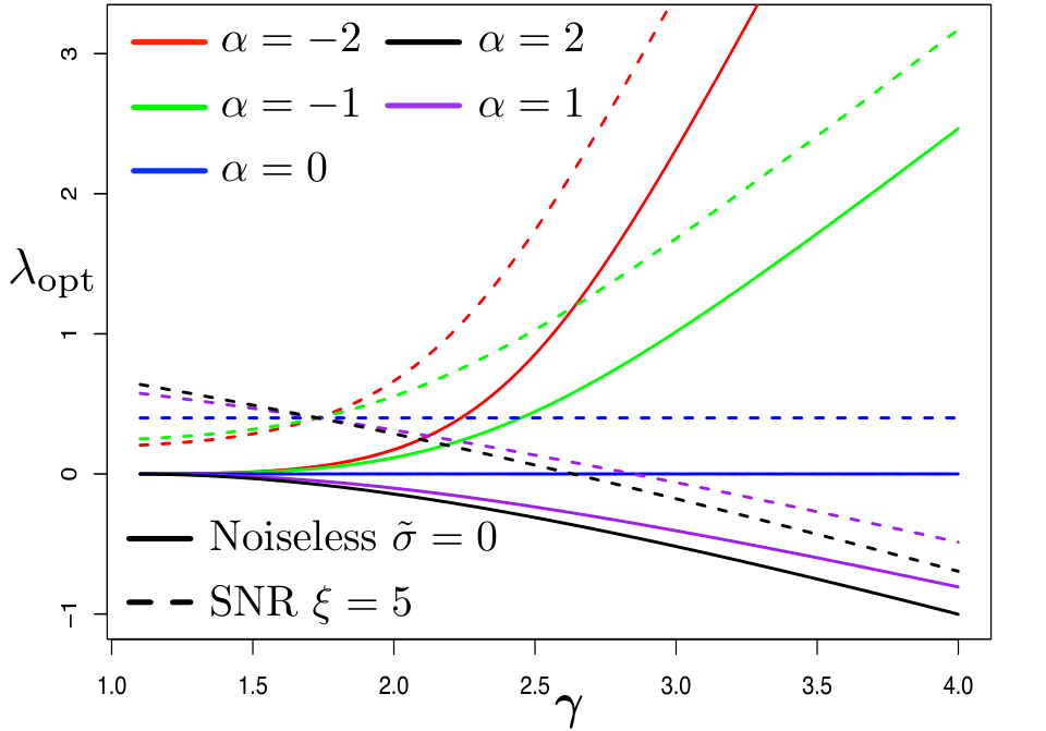
Refer to caption

Left: Optimal Ridge λopt\lambda_{\text{opt}}.

Right: R⁡(λ)R(\lambda): Optimal vs. ridgeless.

Figure 4: We set 𝚺w=𝑰\boldsymbol{\Sigma}_{w}=\boldsymbol{I} and 𝚺β=𝚺xα\boldsymbol{\Sigma}_{\beta}=\boldsymbol{\Sigma}_{x}^{\alpha} where 𝒅x\boldsymbol{d}_{x} has two point masses on 11 and 55 with probability 3/43/4 and 1/41/4 respectively. Left: optimal λ\lambda; solid lines represents the noiseless case σ~=0\tilde{\sigma}=0 and dashed lines represents the noisy case with a fixed SNR ξ=5\xi=5. Right: comparison of prediction risk of the ridgeless (R⁡(λopt)R(\lambda_{\text{opt}}), dashed lines) and optimally regularized (R⁡(λopt)R(\lambda_{\text{opt}}), solid lines) estimator in the noiseless case. We normalize the prediction risk as 𝔼​y~2=𝔼​(𝒙~⊤​𝜷⋆)2\mathbb{E}\tilde{y}^{2}=\mathbb{E}(\tilde{\boldsymbol{x}}^{{\scriptscriptstyle{\top}}}\boldsymbol{\beta}_{\star})^{2}.
  • M1

    λopt<0\lambda_{\text{opt}}<0 when 𝒅x/w\boldsymbol{d}_{x/w} aligns with 𝒅w​β\boldsymbol{d}_{w\beta}, or in general, 𝔼⁡[g|h]\mathbb{E}[g|h] is a strictly increasing function of hh. In the context of standard ridge regression, it means that shrinkage regularization only increases the bias in the overparameterized regime when features are informative, i.e., the projection of the signal is large in the directions where the feature variance is large.

  • M2

    λopt>0\lambda_{\text{opt}}>0 when 𝒅x/w\boldsymbol{d}_{x/w} is misaligned with 𝒅w​β\boldsymbol{d}_{w\beta}, or in general, 𝔼⁡[g|h]\mathbb{E}[g|h] is a strictly decreasing function of hh. This is to say, in standard ridge regression, when features are not informative, i.e., the projection of the signal is small in the directions of large feature variance, shrinkage is beneficial even in the absence of label noise (the variance term is zero).

M1 and M2, together with aforementioned special case when gg and hh have random relation, provide a precise characterization of the sign of λopt\lambda_{\text{opt}}. In particular, M1 confirms the “negative ridge” phenomenon empirically observed in [KLS20] and outlines concise conditions under which it occurs. We emphasize that neither M1 nor M2 would be observed when one of 𝚺x/w\boldsymbol{\Sigma}_{x/w} and 𝚺w​β\boldsymbol{\Sigma}_{w\beta} is identity (as previously discussed). In other words, these observations arise from our more general assumption on (𝚺x/w,𝚺w​β)(\boldsymbol{\Sigma}_{x/w},\boldsymbol{\Sigma}_{w\beta}).

Implicit regularization of overparameterization.

Taking both the bias and variance into account, Theorem 4 demonstrates a bias-variance tradeoff between Part 3 and Part 4, and λopt\lambda_{\text{opt}} will eventually become positive as σ~2\tilde{\sigma}^{2} increases (i.e., the prediction risk is dominated by variance, for which a positive λ\lambda is beneficial). For certain special cases, we can provide a lower bound for the transition from λopt<0\lambda_{\text{opt}}\!<\!0 to λopt>0\lambda_{\text{opt}}\!>\!0.

Proposition 5.

Given Assumption 1, let (h,g)=(1,1)(h,g)=(1,1) with probability 1−q1-q and (h,g)=(h1,g1)(h,g)=(h_{1},g_{1}) with probability qq, where h1>1h_{1}>1 and g1>1g_{1}>1. Denote γ¯=γ−1\bar{\gamma}=\gamma-1. Then λopt<0\lambda_{\text{opt}}<0 if

OPENσ~2<(h1−1)​(g1−1)​h1⋅max⁡((γ​q−1)3​γ¯3​(1−q)OPEN(1−q)​γ2​(γ¯3​q2+(γ​q−1)3​h12CLOSE),γ​q​(1−q)​γ¯3OPEN(1−q)​(h1+γ¯CLOSE)3+q​h12​γ3CLOSE).\tilde{\sigma}^{2}<(h_{1}-1)(g_{1}-1)h_{1}\cdot\max\mathopen{}\mathclose{{\left(\dfrac{(\gamma q-1)^{3}\bar{\gamma}^{3}(1-q)}{(1-q)\gamma^{2}\mathopen{}\mathclose{{\left(\bar{\gamma}^{3}q^{2}+(\gamma q-1)^{3}h_{1}^{2}}}\right)},\dfrac{\gamma q(1-q)\bar{\gamma}^{3}}{(1-q)\mathopen{}\mathclose{{\left(h_{1}+\bar{\gamma}}}\right)^{3}+qh_{1}^{2}\gamma^{3}}}}\right).

As qq approaches 00 or 11, the above upper bound goes to 00 because 𝚺x\boldsymbol{\Sigma}_{x}, 𝚺β\boldsymbol{\Sigma}_{\beta} becomes closer to 𝑰\boldsymbol{I}. Otherwise, when γ​q>1\gamma q>1, the upper bound suggests σ~2=O⁡(g1​γ)\tilde{\sigma}^{2}=O(g_{1}\gamma) which implies that SNR ξ=Ω⁡(h1/γ)\xi=\Omega(h_{1}/\gamma). Hence, as γ\gamma increases, optimal λopt\lambda_{\text{opt}} remains negative for a lower SNR (i.e., larger noise), which coincides with the intuition that overparameterization has an implicit effect of ℓ2\ell_{2} regularization (Figure 4 Left). Indeed, the following proposition suggests such implicit regularization is only significant in the overparameterized regime:

Proposition 6.

When γ<1\gamma<1, λopt\lambda_{\text{opt}} on (−c0,∞)(-c_{0},\infty) is always non-negative under Assumption 1.

Figure 4 confirms our findings in Theorem 4 (for results on different distributions see Figure 10). Specifically, we set OPEN𝚺w=𝑰,𝚺x=diag⁡(𝒅xCLOSE)\boldsymbol{\Sigma}_{w}=\boldsymbol{I},\boldsymbol{\Sigma}_{x}=\operatorname{diag}\mathopen{}\mathclose{{\left(\boldsymbol{d}_{x}}}\right) and 𝚺β=𝚺xα\boldsymbol{\Sigma}_{\beta}=\boldsymbol{\Sigma}_{x}^{\alpha}. As we increase α\alpha from negative to positive, the relation between 𝒅x\boldsymbol{d}_{x} and 𝒅β\boldsymbol{d}_{\beta} transitions from misaligned to aligned. The left panel shows that the sign of λopt\lambda_{\text{opt}} is the exact opposite to the sign of α\alpha in the noiseless case (i.e. the variance is 00), which is consistent with M1 and M2. Moreover, when 𝒅x\boldsymbol{d}_{x} aligns with 𝒅β\boldsymbol{d}_{\beta}, λopt\lambda_{\text{opt}} decreases as γ\gamma becomes larger, which agrees with our observation on the implicit ℓ2\ell_{2} regularization of overparameterization. Last but not least, in Figure 4 (Right) we see that the optimal ridge regression estimator leads to considerable improvement over the ridgeless estimator. We comment that this improvement becomes more significant as γ\gamma or condition number of 𝚺x\boldsymbol{\Sigma}_{x} and 𝚺β\boldsymbol{\Sigma}_{\beta} increases.

Risk monotonicity of optimal ridge regression.

[DS20, Proposition 6] showed that for isotropic data (𝚺x=𝑰\boldsymbol{\Sigma}_{x}=\boldsymbol{I}), the asymptotic prediction risk of optimally-tuned ridge regression monotonically increases with γ\gamma. This is to say, under proper regularization (λ=λopt\lambda=\lambda_{\text{opt}}), increasing the size of training data always helps the test performance. Here we extend this result to data with general covariance and isotropic prior on 𝜷∗\boldsymbol{\beta}_{*}.

Proposition 7.

Given 𝔼⁡[𝐱​𝐱⊤]=𝚺x\mathbb{E}[\boldsymbol{x}\boldsymbol{x}^{\top}]=\boldsymbol{\Sigma}_{x} and 𝔼⁡[𝛃∗​𝛃∗⊤]=cp​𝐈\mathbb{E}[\boldsymbol{\beta}_{*}\boldsymbol{\beta}_{*}^{\top}]=\frac{c}{p}\boldsymbol{I}66 6 Note that the scaling of the parameters differs from the previous setting by γ\gamma to be consistent with that of [DS20]. where 𝚺x\boldsymbol{\Sigma}_{x} satisfies Assumption 1, the prediction risk R⁡(λ)R(\lambda) of the optimally-tuned ridge regression estimator (𝚺w=𝐈\boldsymbol{\Sigma}_{w}=\boldsymbol{I}) with λopt=γ​σ~2/c\lambda_{\mathrm{opt}}=\gamma\tilde{\sigma}^{2}/c is an increasing function of γ∈(0,∞)\gamma\in(0,\infty).

We remark that establishing such characterization under general orientation of 𝜷∗\boldsymbol{\beta}_{*} (anisotropic 𝚺β\boldsymbol{\Sigma}_{\beta}) can be challenging, because the optimal regularization λopt\lambda_{\text{opt}} may not have a convenient closed-form. We leave the analysis for the general case as future work.

6 Optimal Weighting Matrix

Having characterized the optimal regularization strength, we now turn to the optimal choice of weighting matrix 𝚺w\boldsymbol{\Sigma}_{w}. Toward this goal, we additionally require the following assumptions on (𝚺x,𝚺β,𝚺w)(\boldsymbol{\Sigma}_{x},\boldsymbol{\Sigma}_{\beta},\boldsymbol{\Sigma}_{w}):

Assumption 2.

The covariance matrix 𝚺x\boldsymbol{\Sigma}_{x} and the weighting matrix 𝚺w\boldsymbol{\Sigma}_{w} share the same set of eigenvectors, i.e., we have the following eigendecompositions: 𝚺x=𝐔​𝐃x​𝐔⊤\boldsymbol{\Sigma}_{x}=\boldsymbol{U}\boldsymbol{D}_{x}\boldsymbol{U}^{{\scriptscriptstyle{\top}}} and 𝚺w=𝐔​𝐃w​𝐔⊤\boldsymbol{\Sigma}_{w}=\boldsymbol{U}\boldsymbol{D}_{w}\boldsymbol{U}^{{\scriptscriptstyle{\top}}}, where 𝐔∈ℝp×p\boldsymbol{U}\in\mathbb{R}^{p\times p} is orthogonal, and 𝑂𝑃𝐸𝑁𝑂𝑃𝐸𝑁𝐃x=diag⁡(𝐝x𝐶𝐿𝑂𝑆𝐸),𝐃w=diag⁡(𝐝w𝐶𝐿𝑂𝑆𝐸)\boldsymbol{D}_{x}=\operatorname{diag}\mathopen{}\mathclose{{\left(\boldsymbol{d}_{x}}}\right),\boldsymbol{D}_{w}=\operatorname{diag}\mathopen{}\mathclose{{\left(\boldsymbol{d}_{w}}}\right).

We define OPEN𝒅¯β=diag⁡(𝑼⊤​𝚺β​𝑼CLOSE)\bar{\boldsymbol{d}}_{\beta}=\operatorname{diag}\mathopen{}\mathclose{{\left(\boldsymbol{U}^{\scriptscriptstyle{\top}}\boldsymbol{\Sigma}_{\beta}\boldsymbol{U}}}\right). Note that when 𝚺β\boldsymbol{\Sigma}_{\beta} also shares the same eigenvector matrix 𝑼\boldsymbol{U}, then 𝒅¯β=𝒅β\bar{\boldsymbol{d}}_{\beta}=\boldsymbol{d}_{\beta}, which is simply the eigenvalues of 𝚺β\boldsymbol{\Sigma}_{\beta}.

Assumption 3.

Let dx,i,d¯β,i,dw,id_{x,i},\bar{d}_{\beta,i},d_{w,i} be the iith element of 𝐝x,𝐝¯β,𝐝w\boldsymbol{d}_{x},\bar{\boldsymbol{d}}_{\beta},\boldsymbol{d}_{w} respectively. We assume that the empirical distribution of (dx,i,d¯β,i,dw,i)(d_{x,i},\bar{d}_{\beta,i},d_{w,i}) jointly converges to (s,v,s/r)(s,v,s/r), where s,v,rs,v,r are non-negative random variables. Further, there exists constants cl,cu>0c_{l},c_{u}>0 independent of nn and pp such that mini⁡(min⁡(dx,i,d¯β,i,dw,i))≥cl\min_{i}(\min(d_{x,i},\bar{d}_{\beta,i},d_{w,i}))\geq c_{l}, maxi⁡(max⁡(dx,i,d¯β,i,dw,i))≤cu\max_{i}(\max(d_{x,i},\bar{d}_{\beta,i},d_{w,i}))\leq c_{u} and ‖𝚺β‖≤cu\|\boldsymbol{\Sigma}_{\beta}\|\leq c_{u}.

For notational convenience, we define ℋw\mathcal{H}_{w} and ℋr\mathcal{H}_{r} to be the sets of all 𝚺w\boldsymbol{\Sigma}_{w} and rr, respectively, that satisfy Assumption 2 and Assumption 3. Additionally, let 𝒮w\mathcal{S}_{w} and 𝒮r\mathcal{S}_{r} be the subset of ℋw\mathcal{H}_{w} and ℋr\mathcal{H}_{r} such that r=f⁡(s)r=f(s) for some function ff (this represents 𝚺w∈ℋw\boldsymbol{\Sigma}_{w}\in\mathcal{H}_{w} that only depends on 𝚺x\boldsymbol{\Sigma}_{x} but not 𝚺β\boldsymbol{\Sigma}_{\beta}). By Assumption 2 and 3, we know the empirical distribution of (dx/w,i,dw​β,i)(d_{x/w,i},d_{w\beta,i}) jointly converges to (r,s​v/r)(r,sv/r) and satisfies the boundedness requirement in Assumption 1. We therefore apply Theorem 1 to compute the prediction risk:

OPENR⁡(r,λ)≜mr′​(−λ)mr2​(−λ)⋅(γ​𝔼​s​v(r⋅mr​(−λ)+1)2+σ~2CLOSE),\displaystyle R(r,\lambda)\ \triangleq\ \frac{m_{r}^{\prime}(-\lambda)}{m_{r}^{2}(-\lambda)}\cdot\mathopen{}\mathclose{{\left(\gamma\mathbb{E}\frac{sv}{(r\cdot m_{r}(-\lambda)+1)^{2}}+\tilde{\sigma}^{2}}}\right), (6.1)

where mr​(−λ)m_{r}(-\lambda) satisfies the equation λ=mr−1​(−λ)−γ​𝔼​(1+r⋅mr​(−λ))−1​r\lambda=m^{-1}_{r}(-\lambda)-\gamma\mathbb{E}(1+r\cdot m_{r}(-\lambda))^{-1}r. It is clear that when r=a.s.sr\stackrel{{\scriptstyle\text{a.s.}}}{{=}}s, (6.1) reduces to the standard ridge regression with 𝚺w=𝑰\boldsymbol{\Sigma}_{w}=\boldsymbol{I}, and for r=a.s.1r\stackrel{{\scriptstyle\text{a.s.}}}{{=}}1, the equation reduces to the cases of isotropic features (𝚺w=𝚺x\boldsymbol{\Sigma}_{w}=\boldsymbol{\Sigma}_{x}). Note that (6.1) indicates that the impact of 𝚺β\boldsymbol{\Sigma}_{\beta} on the risk is fully captured by 𝒅¯β\bar{\boldsymbol{d}}_{\beta}. Hence we define OPEN𝚺¯β=𝑼​diag⁡(𝒅¯βCLOSE)​𝑼⊤\bar{\boldsymbol{\Sigma}}_{\beta}=\boldsymbol{U}\operatorname{diag}\mathopen{}\mathclose{{\left(\bar{\boldsymbol{d}}_{\beta}}}\right)\boldsymbol{U}^{{\scriptscriptstyle{\top}}}, which corresponds to r=a.s.s​vr\stackrel{{\scriptstyle\text{a.s.}}}{{=}}sv, and is equivalent to 𝚺β\boldsymbol{\Sigma}_{\beta} when 𝚺β\boldsymbol{\Sigma}_{\beta} also shares the same eigenvector matrix 𝑼\boldsymbol{U}. In the following subsections, we discuss the optimal 𝚺w\boldsymbol{\Sigma}_{w} for two types of estimator: the minimum ‖β^‖𝚺w\|\hat{\beta}\|_{\boldsymbol{\Sigma}_{w}} solution (taking λ→0\lambda\to 0), and the optimally-tuned generalized ridge estimator (λ=λopt\lambda=\lambda_{\text{opt}}). Note that the risk for both estimators is scale-invariant over 𝚺w\boldsymbol{\Sigma}_{w} and rr. Hence, when we define a specific choice of (𝚺w,r)(\boldsymbol{\Sigma}_{w},r), we simultaneously consider all pairs (c​𝚺w,r/c)(c\boldsymbol{\Sigma}_{w},\nicefrac{{r}}{{c}}) for c>0c>0. Finally, we note that the choice of r=a.s.s⋅𝔼⁡[v|s]∈𝒮rr\stackrel{{\scriptstyle\text{a.s.}}}{{=}}s\cdot\mathbb{E}[v|s]\in\mathcal{S}_{r} plays a key role in our analysis, and its corresponding choice of 𝚺w\boldsymbol{\Sigma}_{w} is given as OPEN𝚺w=(fv​(𝚺x)CLOSE)−1\boldsymbol{\Sigma}_{w}=\mathopen{}\mathclose{{\left(f_{v}(\boldsymbol{\Sigma}_{x})}}\right)^{-1}, where fv​(s)≜𝔼⁡[v|s]f_{v}(s)\triangleq\mathbb{E}[v|s] and fvf_{v} applies to the eigenvalues of 𝚺x\boldsymbol{\Sigma}_{x}.

6.1 Minimum ‖β^‖𝚺w\|\hat{\beta}\|_{\boldsymbol{\Sigma}_{w}} solution

Taking the ridgeless limit leads to the following bias-variance decomposition of the prediction risk,

Bias:Rb(r)≜mr′​(0)mr2​(0)⋅γ𝔼s​v(r⋅mr​(0)+1)2Variance:Rv(r)≜mr′​(0)mr2​(0)⋅σ~2.\text{Bias:}\quad\text{R}_{\text{b}}(r)\triangleq\frac{m_{r}^{\prime}(0)}{m_{r}^{2}(0)}\cdot\gamma\mathbb{E}\frac{sv}{(r\cdot m_{r}(0)+1)^{2}}\quad\text{Variance:}\quad\text{R}_{\text{v}}(r)\triangleq\frac{m_{r}^{\prime}(0)}{m_{r}^{2}(0)}\cdot\tilde{\sigma}^{2}.

In the previous sections we observe a bias-variance tradeoff in choosing the optimal λ\lambda. Interesting, the following theorem illustrates a similar bias-variance tradeoff in choosing the optimal 𝚺w\boldsymbol{\Sigma}_{w}:

Theorem 8.

Given Assumptions 2 and 3,

  • •

    r=a.s.s​vr\stackrel{{\scriptstyle\text{a.s.}}}{{=}}sv (i.e., 𝚺w=𝚺¯β−1\boldsymbol{\Sigma}_{w}\!=\!\bar{\boldsymbol{\Sigma}}_{\beta}^{-1}) is the optimal choice in ℋr\mathcal{H}_{r} that minimizes the bias function Rb​(r)\text{R}_{\text{b}}(r). Additionally, r=a.s.𝔼⁡[v|s]⋅sr\stackrel{{\scriptstyle\text{a.s.}}}{{=}}\mathbb{E}[v|s]\cdot s (i.e., 𝚺w=(fv​(𝚺x))−1\boldsymbol{\Sigma}_{w}\!=\!(f_{v}(\boldsymbol{\Sigma}_{x}))^{-1}) is the optimal in 𝒮r\mathcal{S}_{r} that minimizes Rb​(r)\text{R}_{\text{b}}(r).

  • •

    r=a.s.1r\stackrel{{\scriptstyle\text{a.s.}}}{{=}}1 (i.e., 𝚺w=𝚺x\boldsymbol{\Sigma}_{w}\!=\!\boldsymbol{\Sigma}_{x}) is the optimal choice in both 𝒮r\mathcal{S}_{r} and ℋr\mathcal{H}_{r} that minimizes the variance Rv​(r)\text{R}_{\text{v}}(r).

Theorem 8 implies that the variance is minimized when 𝚺w=𝚺x\boldsymbol{\Sigma}_{w}=\boldsymbol{\Sigma}_{x}. Since the variance term does not depend on 𝜷⋆\boldsymbol{\beta}_{\star}, it is not surprising that the optimal 𝚺w\boldsymbol{\Sigma}_{w} is also independent of 𝚺β\boldsymbol{\Sigma}_{\beta}. Furthermore, this result is consistent with the intuition that to minimize the variance, β^λ\hat{\beta}_{\lambda} should be penalized more in the higher variance directions of 𝚺x\boldsymbol{\Sigma}_{x}, and vice versa. On the other hand, Theorem 8 also implies that the bias is minimized when 𝒅w=1/𝒅¯β\boldsymbol{d}_{w}=1/\bar{\boldsymbol{d}}_{\beta} which does not depend on 𝒅x\boldsymbol{d}_{x}. While this characterization may not be intuitive, when 𝒅¯β=𝒅β\bar{\boldsymbol{d}}_{\beta}=\boldsymbol{d}_{\beta} (i.e., 𝚺β\boldsymbol{\Sigma}_{\beta} also shares the same eigenvector matrix 𝑼\boldsymbol{U}), one analogy is that since the quadratic regularization corresponds to the a Gaussian prior 𝒩⁡(𝟎,𝚺w−1)\mathcal{N}(\boldsymbol{0},\boldsymbol{\Sigma}_{w}^{-1}), it is reasonable to match 𝚺w−1\boldsymbol{\Sigma}_{w}^{-1} with the covariance of 𝜷⋆\boldsymbol{\beta}_{\star}, which gives the maximum a posteriori (MAP) estimate. In general, the optimal 𝚺w\boldsymbol{\Sigma}_{w} admits a bias-variance tradeoff (i.e., the bias and variance are optimal under different 𝚺w\boldsymbol{\Sigma}_{w}) except for the special case of 𝚺x​𝚺¯β=𝑰\boldsymbol{\Sigma}_{x}\bar{\boldsymbol{\Sigma}}_{\beta}=\boldsymbol{I}.

Additionally, the following proposition demonstrates the advantage of the minimum ‖𝜷^‖𝚺w\|\hat{\boldsymbol{\beta}}\|_{\boldsymbol{\Sigma}_{w}} solution over the PCR estimator in the noiseless case.

Proposition 9.

Under Assumption 2 and 3 and in the noiseless setting σ~=0\tilde{\sigma}=0, suppose ss and 𝔼⁡[v|s]⋅s\mathbb{E}[v|s]\cdot s both have continuous and strictly increasing quantile functions. Then the minimum ‖𝛃^‖𝚺w\|\hat{\boldsymbol{\beta}}\|_{\boldsymbol{\Sigma}_{w}} solution outperforms the PCR estimator for all θ∈[0,1)\theta\in[0,1) when 𝚺w=𝚺¯β−1∈ℋw\boldsymbol{\Sigma}_{w}=\bar{\boldsymbol{\Sigma}}_{\beta}^{-1}\in\mathcal{H}_{w}, or when 𝚺w=(fv​(𝚺x))−1∈𝒮w\boldsymbol{\Sigma}_{w}=(f_{v}(\boldsymbol{\Sigma}_{x}))^{-1}\in\mathcal{S}_{w}.

6.2 Optimal weighted ridge estimator

Finally, we consider the optimally-tuned weighted ridge estimator (λ=λopt\lambda=\lambda_{\text{opt}}) and discuss the optimal choice of weighting matrix 𝚺w\boldsymbol{\Sigma}_{w}.

Theorem 10.

Suppose Assumptions 2 and 3 hold. Then r=a.s.s​vr\stackrel{{\scriptstyle\text{a.s.}}}{{=}}sv (i.e., 𝚺w=𝚺¯β−1\boldsymbol{\Sigma}_{w}\!=\!\bar{\boldsymbol{\Sigma}}_{\beta}^{-1}) is the optimal solution in ℋr\mathcal{H}_{r} that minimizes minλ⁡R⁡(r,λ)\min_{\lambda}R(r,\lambda). Additionally, r=a.s.𝔼⁡[v|s]⋅sr\stackrel{{\scriptstyle\text{a.s.}}}{{=}}\mathbb{E}[v|s]\cdot s (i.e., 𝚺w=(fv​(𝚺x))−1\boldsymbol{\Sigma}_{w}\!=\!(f_{v}(\boldsymbol{\Sigma}_{x}))^{-1}) is the optimal solution in 𝒮r\mathcal{S}_{r} that minimizes minλ⁡R⁡(r,λ)\min_{\lambda}R(r,\lambda).

Refer to caption
Figure 5: R⁡(λopt)/𝔼​(𝒙~⊤​𝜷⋆)2R(\lambda_{\text{opt}})/\mathbb{E}(\tilde{\boldsymbol{x}}^{{\scriptscriptstyle{\top}}}\boldsymbol{\beta}_{\star})^{2} against γ\gamma for various weighting matrix 𝚺w\boldsymbol{\Sigma}_{w}. Solid lines represent the noiseless case σ~=0\tilde{\sigma}=0 and the dashed lines represent the noisy case with fixed SNR ξ\xi. We set 𝒅x\boldsymbol{d}_{x} to be aligned with 𝒅β\boldsymbol{d}_{\beta} and Left: 𝒅x\boldsymbol{d}_{x} to have 4 point masses (1,2,3,4)(1,2,3,4) with equal probabilities and 𝒅β\boldsymbol{d}_{\beta} with 2 point masses on 11 and 55 with probabilities 3/43/4 and 1/41/4, respectively; Right: 𝒅x\boldsymbol{d}_{x} has 2 point masses on 11 and 55 with probabilities 3/43/4 and 1/41/4, respectively, and 𝚺β=𝚺x2\boldsymbol{\Sigma}_{\beta}=\boldsymbol{\Sigma}_{x}^{2}; we set 𝚺w=𝚺βα\boldsymbol{\Sigma}_{w}=\boldsymbol{\Sigma}_{\beta}^{\alpha}.

In contrast to the ridgeless setting in Theorem 8, the optimal 𝒅w\boldsymbol{d}_{w} for the optimally-tuned λopt\lambda_{\text{opt}} does not depend on the noise level but only on 𝒅¯β\bar{\boldsymbol{d}}_{\beta}, the strength of the signal in the directions of the eigenvectors of 𝚺x\boldsymbol{\Sigma}_{x}. One interpretation is that in the optimally weighted estimator, λopt\lambda_{\text{opt}} is capable of balancing the bias-variance tradeoff in the prediction risk; therefore the weighting matrix may not need to adjust to the label noise and can be chosen solely based on the signal 𝜷⋆\boldsymbol{\beta}_{\star}. Indeed, as discussed in the previous section, 𝚺w=𝚺β−1\boldsymbol{\Sigma}_{w}=\boldsymbol{\Sigma}_{\beta}^{-1} is a preferable choice of prior under the Bayesian perspective when 𝒅β=𝒅¯β\boldsymbol{d}_{\beta}=\bar{\boldsymbol{d}}_{\beta}.

Theorem 10 is supported by Figure 5, in which we plot the prediction risk of the generalized ridge regression estimator under different 𝚺w\boldsymbol{\Sigma}_{w} and optimally tuned λopt\lambda_{\text{opt}}. We consider a simple discrete construction for aligned 𝒅x\boldsymbol{d}_{x} and 𝒅β(=𝒅¯β)\boldsymbol{d}_{\beta}(=\bar{\boldsymbol{d}}_{\beta}). On the left panel, we enumerate a few standard choices of 𝚺w\boldsymbol{\Sigma}_{w}: 𝚺x,𝚺β,𝑰,𝚺x−1\boldsymbol{\Sigma}_{x},\boldsymbol{\Sigma}_{\beta},\boldsymbol{I},\boldsymbol{\Sigma}_{x}^{-1} and the optimal choice 𝚺β−1\boldsymbol{\Sigma}_{\beta}^{-1}. On the right, we take 𝚺w\boldsymbol{\Sigma}_{w} to be powers of 𝚺β\boldsymbol{\Sigma}_{\beta} around the optimal 𝚺β−1\boldsymbol{\Sigma}_{\beta}^{-1}. In both setups, we confirm that 𝚺β−1\boldsymbol{\Sigma}_{\beta}^{-1} achieves the lowest risk uniformly over γ\gamma, as predicted by Theorem 10.

Note that our main results generally require knowledge of 𝚺x\boldsymbol{\Sigma}_{x} and 𝚺¯β\bar{\boldsymbol{\Sigma}}_{\beta}. While 𝚺x\boldsymbol{\Sigma}_{x} can be estimated in a semi-supervised setting using unlabeled data (e.g., [RC15, TCG20]), it is typically difficult to estimate 𝚺¯β\bar{\boldsymbol{\Sigma}}_{\beta} directly from data. Without prior knowledge on 𝚺¯β\bar{\boldsymbol{\Sigma}}_{\beta}, Theorem 10 suggests that r=a.s.𝔼⁡[v|s]⋅sr\stackrel{{\scriptstyle\text{a.s.}}}{{=}}\mathbb{E}[v|s]\cdot s is the optimal rr that only depends on ss. That is, 𝚺w=(fv​(𝚺x))−1\boldsymbol{\Sigma}_{w}=(f_{v}(\boldsymbol{\Sigma}_{x}))^{-1} is the optimal 𝚺w\boldsymbol{\Sigma}_{w} that only depends on 𝚺x\boldsymbol{\Sigma}_{x}. In the special case of 𝔼⁡[v|s]=𝔼⁡[v]\mathbb{E}[v|s]=\mathbb{E}[v], the optimal 𝚺w\boldsymbol{\Sigma}_{w} in 𝒮w\mathcal{S}_{w} is equivalent to 𝚺w=𝑰\boldsymbol{\Sigma}_{w}=\boldsymbol{I} (standard ridge regression) due to the scale invariance. When the exact form of fv​(s)f_{v}(s) is also not known, we may use a polynomial or power function of ss to approximate either fv​(s)f_{v}(s) or 1/fv​(s)1/f_{v}(s), whose coefficients can be considered as hyper-parameters and cross-validated. We demonstrate the effectiveness of this heuristic in Figure 6: although our proposed 𝚺w=fv​(𝚺x)−1\boldsymbol{\Sigma}_{w}=f_{v}(\boldsymbol{\Sigma}_{x})^{-1} (blue) is worse than the actual optimal (red) 𝚺w=𝚺β−1\boldsymbol{\Sigma}_{w}=\boldsymbol{\Sigma}_{\beta}^{-1} (same as 𝚺¯β−1\bar{\boldsymbol{\Sigma}}_{\beta}^{-1} due to diagonal design), it is the best choice among weighting matrices that only depend on 𝚺x\boldsymbol{\Sigma}_{x}. In addition, we seek the best approximation of fv​(s)f_{v}(s) by applying a power transformation on 𝚺x\boldsymbol{\Sigma}_{x}, and we observe that certain powers of 𝚺x\boldsymbol{\Sigma}_{x} also outperform the standard isotropic regularization.

Refer to caption
Refer to caption
Figure 6: R⁡(λopt)/𝔼​(𝒙~⊤​𝜷⋆)2R(\lambda_{\text{opt}})/\mathbb{E}(\tilde{\boldsymbol{x}}^{{\scriptscriptstyle{\top}}}\boldsymbol{\beta}_{\star})^{2} against γ\gamma for various weighting matrix 𝚺w\boldsymbol{\Sigma}_{w} under noiseless σ~=0\tilde{\sigma}=0 (solid lines) and noisy setting with fixed SNR ξ\xi (dashed lines). Left: We set fv​(s)f_{v}(s) as an increasing function of ss on its support; Right: We set fv​(s)f_{v}(s) as a decreasing function of ss on its support. Note that the heuristically chosen weighting matrices often outperform the standard ridge regression estimator (green).

7 Conclusion

Figure 7: vanishing or negative regularization can be beneficial in certain two-layer neural nets.

We provide a precise asymptotic characterization of the prediction risk of the generalized ridge regression estimator in the overparameterized regime. Our result greatly extends previous high-dimensional analysis of ridge regression, and enables us to discover and theoretically justify various interesting findings, including the negative ridge phenomenon, the implicit regularization of overparameterization, and a concise description of the optimal weighted ridge penalty. We remark that some assumptions in our derivation may be further relaxed; for instance, the bounded eigenvalue assumption can be relaxed to certain polynomial decay (e.g., see [XH19]). We also believe that similar findings can be observed in more complicated models, such as random features regression (see red line in Figure 7). Another fruitful direction is to construct weighting matrix 𝚺w\boldsymbol{\Sigma}_{w} solely from training data that outperforms isotropic shrinkage in the overparameterized regime.

Acknowledgement

The authors would like to thank Murat A. Erdogdu, Daniel Hsu and Taiji Suzuki for comments and suggestions, and also anonymous NeurIPS reviewers 1 and 3 for helpful feedback. DW was partially funded by CIFAR, NSERC and LG Electronics. JX was supported by a Cheung-Kong Graduate School of Business Fellowship.

References

  • [ABG+20] Shun-ichi Amari, Jimmy Ba, Roger Grosse, Xuechen Li, Atsushi Nitanda, Taiji Suzuki, Denny Wu, and Ji Xu, When does preconditioning help or hurt generalization?, arXiv preprint arXiv:2006.10732 (2020).
  • [AKT19] Alnur Ali, J Zico Kolter, and Ryan J Tibshirani, A continuous-time view of early stopping for least squares, International Conference on Artificial Intelligence and Statistics, vol. 22, 2019.
  • [AS17] Madhu S Advani and Andrew M Saxe, High-dimensional dynamics of generalization error in neural networks, arXiv preprint arXiv:1710.03667 (2017).
  • [BES+20] Jimmy Ba, Murat Erdogdu, Taiji Suzuki, Denny Wu, and Tianzong Zhang, Generalization of two-layer neural networks: An asymptotic viewpoint, International Conference on Learning Representations, 2020.
  • [BHMM18] Mikhail Belkin, Daniel Hsu, Siyuan Ma, and Soumik Mandal, Reconciling modern machine learning and the bias-variance trade-off, arXiv preprint arXiv:1812.11118 (2018).
  • [BHX19] Mikhail Belkin, Daniel Hsu, and Ji Xu, Two models of double descent for weak features, arXiv preprint arXiv:1903.07571 (2019).
  • [BLLT19] Peter L Bartlett, Philip M Long, Gábor Lugosi, and Alexander Tsigler, Benign overfitting in linear regression, arXiv preprint arXiv:1906.11300 (2019).
  • [BS99] Anders Björkström and Rolf Sundberg, A generalized view on continuum regression, Scandinavian Journal of Statistics 26 (1999), no. 1, 17–30.
  • [BVDBS+15] Małgorzata Bogdan, Ewout Van Den Berg, Chiara Sabatti, Weijie Su, and Emmanuel J Candès, Slope—adaptive variable selection via convex optimization, The annals of applied statistics 9 (2015), no. 3, 1103.
  • [Cas80] George Casella, Minimax ridge regression estimation, The Annals of Statistics (1980), 1036–1056.
  • [CWB08] Emmanuel J Candes, Michael B Wakin, and Stephen P Boyd, Enhancing sparsity by reweighted ℓ1\ell_{1} minimization, Journal of Fourier analysis and applications 14 (2008), no. 5-6, 877–905.
  • [Dic16] Lee H Dicker, Ridge regression and asymptotic minimax estimation over spheres of growing dimension, Bernoulli 22 (2016), no. 1, 1–37.
  • [DKT19] Zeyu Deng, Abla Kammoun, and Christos Thrampoulidis, A model of double descent for high-dimensional binary linear classification, arXiv preprint arXiv:1911.05822 (2019).
  • [DLM19] Michał Dereziński, Feynman Liang, and Michael W Mahoney, Exact expressions for double descent and implicit regularization via surrogate random design, arXiv preprint arXiv:1912.04533 (2019).
  • [DM16] David Donoho and Andrea Montanari, High dimensional robust m-estimation: Asymptotic variance via approximate message passing, Probability Theory and Related Fields 166 (2016), no. 3-4, 935–969.
  • [dRBK20] Stéphane d’Ascoli, Maria Refinetti, Giulio Biroli, and Florent Krzakala, Double trouble in double descent: Bias and variance (s) in the lazy regime, arXiv preprint arXiv:2003.01054 (2020).
  • [DS20] Edgar Dobriban and Yue Sheng, Wonder: Weighted one-shot distributed ridge regression in high dimensions., Journal of Machine Learning Research 21 (2020), no. 66, 1–52.
  • [DW18] Edgar Dobriban and Stefan Wager, High-dimensional asymptotics of prediction: Ridge regression and classification, The Annals of Statistics 46 (2018), no. 1, 247–279.
  • [HG83] Tsushung A Hua and Richard F Gunst, Generalized ridge regression: a note on negative ridge parameters, Communications in Statistics-Theory and Methods 12 (1983), no. 1, 37–45.
  • [HK70] Arthur E Hoerl and Robert W Kennard, Ridge regression: Biased estimation for nonorthogonal problems, Technometrics 12 (1970), no. 1, 55–67.
  • [HL20] Hong Hu and Yue M Lu, Universality laws for high-dimensional learning with random features, arXiv preprint arXiv:2009.07669 (2020).
  • [HMRT19] Trevor Hastie, Andrea Montanari, Saharon Rosset, and Ryan J Tibshirani, Surprises in high-dimensional ridgeless least squares interpolation, arXiv preprint arXiv:1903.08560 (2019).
  • [Kar13] Noureddine El Karoui, Asymptotic behavior of unregularized and ridge-regularized high-dimensional robust regression estimators: rigorous results, arXiv preprint arXiv:1311.2445 (2013).
  • [KH92] Anders Krogh and John A Hertz, A simple weight decay can improve generalization, Advances in neural information processing systems, 1992, pp. 950–957.
  • [KLS20] Dmitry Kobak, Jonathan Lomond, and Benoit Sanchez, The optimal ridge penalty for real-world high-dimensional data can be zero or negative due to the implicit ridge regularization, Journal of Machine Learning Research 21 (2020), no. 169, 1–16.
  • [KPR+17] James Kirkpatrick, Razvan Pascanu, Neil Rabinowitz, Joel Veness, Guillaume Desjardins, Andrei A Rusu, Kieran Milan, John Quan, Tiago Ramalho, Agnieszka Grabska-Barwinska, et al., Overcoming catastrophic forgetting in neural networks, Proceedings of the national academy of sciences 114 (2017), no. 13, 3521–3526.
  • [LD19] Sifan Liu and Edgar Dobriban, Ridge regression: Structure, cross-validation, and sketching, arXiv preprint arXiv:1910.02373 (2019).
  • [LH17] Ilya Loshchilov and Frank Hutter, Decoupled weight decay regularization, arXiv preprint arXiv:1711.05101 (2017).
  • [Lol20] Panagiotis Lolas, Regularization in high-dimensional regression and classification via random matrix theory, arXiv preprint arXiv:2003.13723 (2020).
  • [LP11] Olivier Ledoit and Sandrine Péché, Eigenvectors of some large sample covariance matrix ensembles, Probability Theory and Related Fields 151 (2011), no. 1-2, 233–264.
  • [LPRS17] Tengyuan Liang, Tomaso Poggio, Alexander Rakhlin, and James Stokes, Fisher-rao metric, geometry, and complexity of neural networks, arXiv preprint arXiv:1711.01530 (2017).
  • [LW17] Christos Louizos and Max Welling, Multiplicative normalizing flows for variational bayesian neural networks, Proceedings of the 34th International Conference on Machine Learning-Volume 70, JMLR. org, 2017, pp. 2218–2227.
  • [MM19] Song Mei and Andrea Montanari, The generalization error of random features regression: Precise asymptotics and double descent curve, arXiv preprint arXiv:1908.05355 (2019).
  • [MRSY19] Andrea Montanari, Feng Ruan, Youngtak Sohn, and Jun Yan, The generalization error of max-margin linear classifiers: High-dimensional asymptotics in the overparametrized regime, arXiv preprint arXiv:1911.01544 (2019).
  • [MS05] Yuzo Maruyama and William E Strawderman, A new class of generalized bayes minimax ridge regression estimators, The Annals of Statistics 33 (2005), no. 4, 1753–1770.
  • [MS18] Yuichi Mori and Taiji Suzuki, Generalized ridge estimator and model selection criteria in multivariate linear regression, Journal of Multivariate Analysis 165 (2018), 243–261.
  • [RC15] Kenneth Joseph Ryan and Mark Vere Culp, On semi-supervised linear regression in covariate shift problems, The Journal of Machine Learning Research 16 (2015), no. 1, 3183–3217.
  • [RM11] Francisco Rubio and Xavier Mestre, Spectral convergence for a general class of random matrices, Statistics & probability letters 81 (2011), no. 5, 592–602.
  • [RMR20] Dominic Richards, Jaouad Mourtada, and Lorenzo Rosasco, Asymptotics of ridge (less) regression under general source condition, arXiv preprint arXiv:2006.06386 (2020).
  • [SC95] Jack W Silverstein and Sang-Il Choi, Analysis of the limiting spectral distribution of large dimensional random matrices, Journal of Multivariate Analysis 54 (1995), no. 2, 295–309.
  • [Str78] William E Strawderman, Minimax adaptive generalized ridge regression estimators, Journal of the American Statistical Association 73 (1978), no. 363, 623–627.
  • [TAH18] Christos Thrampoulidis, Ehsan Abbasi, and Babak Hassibi, Precise error analysis of regularized mm-estimators in high dimensions, IEEE Transactions on Information Theory 64 (2018), no. 8, 5592–5628.
  • [TB20] Alexander Tsigler and Peter L Bartlett, Benign overfitting in ridge regression, arXiv preprint arXiv:2009.14286 (2020).
  • [TCG20] T Tony Cai and Zijian Guo, Semisupervised inference for explained variance in high dimensional linear regression and its applications, Journal of the Royal Statistical Society: Series B (Statistical Methodology) (2020).
  • [XH19] Ji Xu and Daniel J Hsu, On the number of variables to use in principal component regression, Advances in Neural Information Processing Systems, 2019, pp. 5095–5104.
  • [Zou06] Hui Zou, The adaptive lasso and its oracle properties, Journal of the American statistical association 101 (2006), no. 476, 1418–1429.
  • [ZTSG19] Han Zhao, Yao-Hung Hubert Tsai, Russ R Salakhutdinov, and Geoffrey J Gordon, Learning neural networks with adaptive regularization, Advances in Neural Information Processing Systems, 2019, pp. 11389–11400.
  • [ZWXG18] Guodong Zhang, Chaoqi Wang, Bowen Xu, and Roger Grosse, Three mechanisms of weight decay regularization, arXiv preprint arXiv:1810.12281 (2018).

Appendix A Proofs omitted in Section 4

A.1 Proof of Theorem 1

We first claim that function m⁡(−λ)m(-\lambda) that satisfies (4.2) is indeed the Stieltjes transform of the limiting distribution of the eigenvalues of 𝑿/w​𝑿/w⊤\boldsymbol{X}_{/w}\boldsymbol{X}_{/w}^{{\scriptscriptstyle{\top}}}. This is because the empirical distribution of the eigenvalues of 𝚺x/w\boldsymbol{\Sigma}_{x/w} converges to the distribution of hh due to Assumption 1. By the Marchenko-Pastur law, it is straightforward to show that the minimal eigenvalue of 𝑿/w​𝑿/w⊤\boldsymbol{X}_{/w}\boldsymbol{X}_{/w}^{{\scriptscriptstyle{\top}}} is lower bounded by c0c_{0} as n→∞n\to\infty. Hence, we have m⁡(−λ)>0m(-\lambda)>0 for all λ>−c0\lambda>-c_{0}. Then by taking derivatives of (4.2)77 7 We can exchange expectation and derivatives because |∂h1+h​m∂m|=h(1+h​m)2<suph\mathopen{}\mathclose{{\left|\frac{\partial\frac{h}{1+hm}}{\partial m}}}\right|=\frac{h}{(1+hm)^{2}}<\sup h when m⁡(−λ)>0m(-\lambda)>0, we know that (4.3) holds. The rest of the proof is to characterize Part 1 and Part 2 in (3.1) and show (4.1).

For Part 1 in (3.1), based on prior works [DW18, XH19], we have

Part 1 in (3.1)→pσ~2​m′​(−λ)m2​(−λ).\displaystyle\text{Part 1 in \eqref{eq:risk_eq1}}\ \stackrel{{\scriptstyle\text{p}}}{{\rightarrow}}\ \tilde{\sigma}^{2}\frac{m^{\prime}(-\lambda)}{m^{2}(-\lambda)}. (A.1)

Hence, we only need to show that

Part 2 in (3.1)→pm′​(−λ)m2​(−λ)⋅γ​𝔼​g​h(h⋅m⁡(−λ)+1)2.\displaystyle\text{Part 2 in \eqref{eq:risk_eq1}}\ \stackrel{{\scriptstyle\text{p}}}{{\rightarrow}}\ \frac{m^{\prime}(-\lambda)}{m^{2}(-\lambda)}\cdot\gamma\mathbb{E}\frac{gh}{(h\cdot m(-\lambda)+1)^{2}}. (A.2)

Towards this goal, we first assume that 𝚺w​β\boldsymbol{\Sigma}_{w\beta} is invertible and define 𝑺=𝑿/w2​β⊤​𝑿/w2​β+λ​𝚺w​β−1\boldsymbol{S}=\boldsymbol{X}_{/w^{2}\beta}^{{\scriptscriptstyle{\top}}}\boldsymbol{X}_{/w^{2}\beta}+\lambda\boldsymbol{\Sigma}_{w\beta}^{-1}, where 𝑿/w2​β=𝑿/w𝚺w​β−1/2∼𝒩(0,1n​𝚺x/w2​βCLOSE)\boldsymbol{X}_{/w^{2}\beta}=\boldsymbol{X}_{/w}\boldsymbol{\Sigma}_{w\beta}^{-1/2}\sim\mathcal{N}\mathopen{}\mathclose{{\left(0,\frac{1}{n}\boldsymbol{\Sigma}_{x/w^{2}\beta}}}\right) and 𝚺x/w2​β=𝚺w​β−1/2𝚺x/w𝚺w​β−1/2\boldsymbol{\Sigma}_{x/w^{2}\beta}=\boldsymbol{\Sigma}_{w\beta}^{-1/2}\boldsymbol{\Sigma}_{x/w}\boldsymbol{\Sigma}_{w\beta}^{-1/2}. Simplification of Part 2 yields

OPENλ2n​tr⁡(𝚺x/w2​β​𝑺−2CLOSE).\frac{\lambda^{2}}{n}\operatorname{tr}\mathopen{}\mathclose{{\left(\boldsymbol{\Sigma}_{x/w^{2}\beta}\boldsymbol{S}^{-2}}}\right).

To analyze the above quantity, we adopt the similar strategy used in [LP11] and first characterize a related quantity OPEN1n​tr⁡(𝑿/w2​β⊤​𝑿/w​β2CLOSE)\frac{1}{n}\operatorname{tr}\mathopen{}\mathclose{{\left(\boldsymbol{X}_{/w^{2}\beta}^{{\scriptscriptstyle{\top}}}\boldsymbol{X}_{/w\beta^{2}}}}\right). Note that, on one hand, we know that

OPEN1n​tr⁡(𝑺−2​𝑿/w2​β⊤​𝑿/w2​βCLOSE)\displaystyle\frac{1}{n}\operatorname{tr}\mathopen{}\mathclose{{\left(\boldsymbol{S}^{-2}\boldsymbol{X}_{/w^{2}\beta}^{{\scriptscriptstyle{\top}}}\boldsymbol{X}_{/w^{2}\beta}}}\right) =\displaystyle= OPEN1n​tr⁡(𝑺−1−λ​𝑺−2​𝚺w​β−1CLOSE)\displaystyle\frac{1}{n}\operatorname{tr}\mathopen{}\mathclose{{\left(\boldsymbol{S}^{-1}-\lambda\boldsymbol{S}^{-2}\boldsymbol{\Sigma}_{w\beta}^{-1}}}\right) (A.3)
=\displaystyle= OPEN1n​tr⁡(𝚺w​β​(𝑿/w⊤​𝑿/w+λ​𝑰)−1−λ​𝚺w​β​(𝑿/w⊤​𝑿/w+λ​𝑰)−2CLOSE).\displaystyle\frac{1}{n}\operatorname{tr}\mathopen{}\mathclose{{\left(\boldsymbol{\Sigma}_{w\beta}(\boldsymbol{X}_{/w}^{{\scriptscriptstyle{\top}}}\boldsymbol{X}_{/w}+\lambda\boldsymbol{I})^{-1}-\lambda\boldsymbol{\Sigma}_{w\beta}(\boldsymbol{X}_{/w}^{{\scriptscriptstyle{\top}}}\boldsymbol{X}_{/w}+\lambda\boldsymbol{I})^{-2}}}\right).

On the other hand, let 𝒙/w2​β,i\boldsymbol{x}_{/w^{2}\beta,i} be the iith row of 𝑿/w2​β\boldsymbol{X}_{/w^{2}\beta} and 𝑺\i=𝑺−𝒙/w2​β,i​𝒙/w2​β,i⊤\boldsymbol{S}_{\backslash i}=\boldsymbol{S}-\boldsymbol{x}_{/w^{2}\beta,i}\boldsymbol{x}_{/w^{2}\beta,i}^{{\scriptscriptstyle{\top}}}, then we have

OPEN1n​tr⁡(𝑺−2​𝑿/w2​β⊤​𝑿/w2​βCLOSE)\displaystyle\frac{1}{n}\operatorname{tr}\mathopen{}\mathclose{{\left(\boldsymbol{S}^{-2}\boldsymbol{X}_{/w^{2}\beta}^{{\scriptscriptstyle{\top}}}\boldsymbol{X}_{/w^{2}\beta}}}\right) =\displaystyle= 1n​∑i=1n𝒙/w2​β,i⊤​𝑺−2​𝒙/w2​β,i=1n​∑i=1nλ2​𝒙/w2​β,i⊤​𝑺\i−2​𝒙/w2​β,iOPEN(λ+λ​𝒙/w2​β,i⊤​𝑺\i−1​𝒙/w2​β,iCLOSE)2,\displaystyle\frac{1}{n}\sum_{i=1}^{n}\boldsymbol{x}_{/w^{2}\beta,i}^{{\scriptscriptstyle{\top}}}\boldsymbol{S}^{-2}\boldsymbol{x}_{/w^{2}\beta,i}\ =\ \frac{1}{n}\sum_{i=1}^{n}\frac{\lambda^{2}\boldsymbol{x}_{/w^{2}\beta,i}^{{\scriptscriptstyle{\top}}}\boldsymbol{S}^{-2}_{\backslash i}\boldsymbol{x}_{/w^{2}\beta,i}}{\mathopen{}\mathclose{{\left(\lambda+\lambda\boldsymbol{x}_{/w^{2}\beta,i}^{{\scriptscriptstyle{\top}}}\boldsymbol{S}^{-1}_{\backslash i}\boldsymbol{x}_{/w^{2}\beta,i}}}\right)^{2}}, (A.4)

where the last equality holds due to the Matrix Inversion Lemma. Note that from Assumption 1, the eigenvalues of 𝚺x/w\boldsymbol{\Sigma}_{x/w} is lower bounded and upper bounded away from 00 and ∞\infty. Also, ‖𝚺w​β‖\|\boldsymbol{\Sigma}_{w\beta}\| is bounded away from ∞\infty. Hence, by the Marchenko–Pastur law, we know that

‖λ2𝚺x/w1/2𝚺w​β−1/2S\i−2𝚺w​β−1/2𝚺x/w1/2‖=‖λ2𝚺x/w1/2(𝑿/w⊤𝑿/w+λ𝑰)−1𝚺w​β(𝑿/w⊤𝑿/w+λ𝑰)−1𝚺x/w1/2‖\mathopen{}\mathclose{{\left\|\lambda^{2}\boldsymbol{\Sigma}_{x/w}^{1/2}\boldsymbol{\Sigma}_{w\beta}^{-1/2}S_{\backslash i}^{-2}\boldsymbol{\Sigma}_{w\beta}^{-1/2}\boldsymbol{\Sigma}_{x/w}^{1/2}}}\right\|=\mathopen{}\mathclose{{\left\|\lambda^{2}\boldsymbol{\Sigma}_{x/w}^{1/2}(\boldsymbol{X}_{/w}^{{\scriptscriptstyle{\top}}}\boldsymbol{X}_{/w}+\lambda\boldsymbol{I})^{-1}\boldsymbol{\Sigma}_{w\beta}(\boldsymbol{X}_{/w}^{{\scriptscriptstyle{\top}}}\boldsymbol{X}_{/w}+\lambda\boldsymbol{I})^{-1}\boldsymbol{\Sigma}_{x/w}^{1/2}}}\right\|

and

‖λ𝚺x/w1/2𝚺w​β−1/2S\i−1𝚺w​β−1/2𝚺x/w1/2‖=‖λ𝚺x/w1/2(𝑿/w⊤𝑿/w+λ𝑰)−1𝚺x/w1/2‖\mathopen{}\mathclose{{\left\|\lambda\boldsymbol{\Sigma}_{x/w}^{1/2}\boldsymbol{\Sigma}_{w\beta}^{-1/2}S_{\backslash i}^{-1}\boldsymbol{\Sigma}_{w\beta}^{-1/2}\boldsymbol{\Sigma}_{x/w}^{1/2}}}\right\|=\mathopen{}\mathclose{{\left\|\lambda\boldsymbol{\Sigma}_{x/w}^{1/2}(\boldsymbol{X}_{/w}^{{\scriptscriptstyle{\top}}}\boldsymbol{X}_{/w}+\lambda\boldsymbol{I})^{-1}\boldsymbol{\Sigma}_{x/w}^{1/2}}}\right\|

are upper bounded away from ∞\infty for any λ>−c0\lambda>-c_{0}88 8 We take pseudo-inverse when λ=0\lambda=0. Furthermore, observe that 𝒙/w2​β,i\boldsymbol{x}_{/w^{2}\beta,i} is independent of 𝑺\i\boldsymbol{S}_{\backslash i} and(A.4). Hence by Lemma 2.1 in [LP11], we can show that

OPEN1n​tr⁡(𝑺−2​𝑿/w2​β⊤​𝑿/w2​βCLOSE)\displaystyle\frac{1}{n}\operatorname{tr}\mathopen{}\mathclose{{\left(\boldsymbol{S}^{-2}\boldsymbol{X}_{/w^{2}\beta}^{{\scriptscriptstyle{\top}}}\boldsymbol{X}_{/w^{2}\beta}}}\right) →p\displaystyle\stackrel{{\scriptstyle\text{p}}}{{\rightarrow}} 1n​∑i=1nOPENλ2n​tr⁡(𝚺x/w2​β​𝑺\i−2CLOSE)OPEN(λ+λn​tr⁡(𝚺x/w2​β​𝑺\i−1CLOSE))2,∀λ>−c0.\displaystyle\frac{1}{n}\sum_{i=1}^{n}\frac{\frac{\lambda^{2}}{n}\operatorname{tr}\mathopen{}\mathclose{{\left(\boldsymbol{\Sigma}_{x/w^{2}\beta}\boldsymbol{S}_{\backslash i}^{-2}}}\right)}{\mathopen{}\mathclose{{\left(\lambda+\frac{\lambda}{n}\operatorname{tr}\mathopen{}\mathclose{{\left(\boldsymbol{\Sigma}_{x/w^{2}\beta}\boldsymbol{S}_{\backslash i}^{-1}}}\right)}}\right)^{2}},\ \forall\lambda>-c_{0}.

Next, we replace 𝑺\i−1\boldsymbol{S}_{\backslash i}^{-1} by 𝑺−1\boldsymbol{S}^{-1} and show the difference made by this rank-1 perturbation is negligible. From the Matrix Inversion Lemma, we have

supi|λntr(𝚺x/w2​β​𝑺\i−1CLOSE)−λntr(𝚺x/w2​β​𝑺−1CLOSE)|\displaystyle\sup_{i}\mathopen{}\mathclose{{\left|\frac{\lambda}{n}\operatorname{tr}\mathopen{}\mathclose{{\left(\boldsymbol{\Sigma}_{x/w^{2}\beta}\boldsymbol{S}_{\backslash i}^{-1}}}\right)-\frac{\lambda}{n}\operatorname{tr}\mathopen{}\mathclose{{\left(\boldsymbol{\Sigma}_{x/w^{2}\beta}\boldsymbol{S}^{-1}}}\right)}}\right|
=\displaystyle= supiλn​𝒙/w2​β,i⊤​𝑺\i−1​𝚺x/w2​β​𝑺\i−1​𝒙/w2​β,i1+𝒙/w2​β,i⊤​𝑺\i−1​𝒙/w2​β,i\displaystyle\sup_{i}\frac{\lambda}{n}\frac{\boldsymbol{x}_{/w^{2}\beta,i}^{{\scriptscriptstyle{\top}}}\boldsymbol{S}_{\backslash i}^{-1}\boldsymbol{\Sigma}_{x/w^{2}\beta}\boldsymbol{S}_{\backslash i}^{-1}\boldsymbol{x}_{/w^{2}\beta,i}}{1+\boldsymbol{x}_{/w^{2}\beta,i}^{{\scriptscriptstyle{\top}}}\boldsymbol{S}_{\backslash i}^{-1}\boldsymbol{x}_{/w^{2}\beta,i}}
≤\displaystyle\leq supiλn​∥𝒙/w2​β,i⊤𝑺\i−1𝚺x/w2​β𝑺\i−1/2∥⋅∥𝑺\i−1/2𝒙/w2​β,i∥1+𝒙/w2​β,i⊤​𝑺\i−1​𝒙/w2​β,i\displaystyle\sup_{i}\frac{\lambda}{n}\frac{\|\boldsymbol{x}_{/w^{2}\beta,i}^{{\scriptscriptstyle{\top}}}\boldsymbol{S}_{\backslash i}^{-1}\boldsymbol{\Sigma}_{x/w^{2}\beta}\boldsymbol{S}_{\backslash i}^{-1/2}\|\cdot\|\boldsymbol{S}_{\backslash i}^{-1/2}\boldsymbol{x}_{/w^{2}\beta,i}\|}{1+\boldsymbol{x}_{/w^{2}\beta,i}^{{\scriptscriptstyle{\top}}}\boldsymbol{S}_{\backslash i}^{-1}\boldsymbol{x}_{/w^{2}\beta,i}}
≤\displaystyle\leq supiλn​∥𝒙/w2​β,i⊤𝑺\i−1/2∥⋅∥𝑺\i−1/2𝚺x/w2​β𝑺\i−1/2∥⋅∥𝑺\i−1/2𝒙/w2​β,i∥1+𝒙/w2​β,i⊤​𝑺\i−1​𝒙/w2​β,i\displaystyle\sup_{i}\frac{\lambda}{n}\frac{\|\boldsymbol{x}_{/w^{2}\beta,i}^{{\scriptscriptstyle{\top}}}\boldsymbol{S}_{\backslash i}^{-1/2}\|\cdot\|\boldsymbol{S}_{\backslash i}^{-1/2}\boldsymbol{\Sigma}_{x/w^{2}\beta}\boldsymbol{S}_{\backslash i}^{-1/2}\|\cdot\|\boldsymbol{S}_{\backslash i}^{-1/2}\boldsymbol{x}_{/w^{2}\beta,i}\|}{1+\boldsymbol{x}_{/w^{2}\beta,i}^{{\scriptscriptstyle{\top}}}\boldsymbol{S}_{\backslash i}^{-1}\boldsymbol{x}_{/w^{2}\beta,i}}
≤\displaystyle\leq ∥𝚺x/w∥⋅supiλ‖(𝑿/w⊤​𝑿/w+λ​𝑰−𝒙/w,i​𝒙/w,i⊤CLOSE)−1‖⋅supi1n𝒙/w2​β,i⊤​𝑺\i−1​𝒙/w2​β,i1+𝒙/w2​β,i⊤​𝑺\i−1​𝒙/w2​β,i\displaystyle\|\boldsymbol{\Sigma}_{x/w}\|\cdot\sup_{i}\lambda\mathopen{}\mathclose{{\left\|\mathopen{}\mathclose{{\left(\boldsymbol{X}_{/w}^{{\scriptscriptstyle{\top}}}\boldsymbol{X}_{/w}+\lambda\boldsymbol{I}-\boldsymbol{x}_{/w,i}\boldsymbol{x}_{/w,i}^{{\scriptscriptstyle{\top}}}}}\right)^{-1}}}\right\|\cdot\sup_{i}\frac{1}{n}\frac{\boldsymbol{x}_{/w^{2}\beta,i}^{{\scriptscriptstyle{\top}}}\boldsymbol{S}_{\backslash i}^{-1}\boldsymbol{x}_{/w^{2}\beta,i}}{1+\boldsymbol{x}_{/w^{2}\beta,i}^{{\scriptscriptstyle{\top}}}\boldsymbol{S}_{\backslash i}^{-1}\boldsymbol{x}_{/w^{2}\beta,i}}
≤\displaystyle\leq OPENOp​(1nCLOSE).\displaystyle O_{\text{p}}\mathopen{}\mathclose{{\left(\frac{1}{n}}}\right).

Similarly,

supi|λ2ntr(𝚺x/w2​β​𝑺\i−2CLOSE)−λ2ntr(𝚺x/w2​β​𝑺−2CLOSE)|\displaystyle\sup_{i}\mathopen{}\mathclose{{\left|\frac{\lambda^{2}}{n}\operatorname{tr}\mathopen{}\mathclose{{\left(\boldsymbol{\Sigma}_{x/w^{2}\beta}\boldsymbol{S}_{\backslash i}^{-2}}}\right)-\frac{\lambda^{2}}{n}\operatorname{tr}\mathopen{}\mathclose{{\left(\boldsymbol{\Sigma}_{x/w^{2}\beta}\boldsymbol{S}^{-2}}}\right)}}\right|
=\displaystyle= supi|λ2ntr(𝚺x/w2​β​𝑺\i−1​(𝑺\i−1−𝑺−1CLOSE))|+supi|λ2ntr(𝚺x/w2​β​(𝑺\i−1−𝑺−1CLOSE)​𝑺−1)|\displaystyle\sup_{i}\mathopen{}\mathclose{{\left|\frac{\lambda^{2}}{n}\operatorname{tr}\mathopen{}\mathclose{{\left(\boldsymbol{\Sigma}_{x/w^{2}\beta}\boldsymbol{S}_{\backslash i}^{-1}\mathopen{}\mathclose{{\left(\boldsymbol{S}_{\backslash i}^{-1}-\boldsymbol{S}^{-1}}}\right)}}\right)}}\right|+\sup_{i}\mathopen{}\mathclose{{\left|\frac{\lambda^{2}}{n}\operatorname{tr}\mathopen{}\mathclose{{\left(\boldsymbol{\Sigma}_{x/w^{2}\beta}\mathopen{}\mathclose{{\left(\boldsymbol{S}_{\backslash i}^{-1}-\boldsymbol{S}^{-1}}}\right)\boldsymbol{S}^{-1}}}\right)}}\right|
≤\displaystyle\leq OPEN‖𝚺x/w‖⋅‖𝚺w​β‖​(supiλ‖(𝑿/w⊤​𝑿/w+λ​𝑰−𝒙/w,i​𝒙/w,i⊤CLOSE)−1‖+λ‖(𝑿/w⊤​𝑿/w+λ​𝑰CLOSE)−1‖)\displaystyle\|\boldsymbol{\Sigma}_{x/w}\|\cdot\|\boldsymbol{\Sigma}_{w\beta}\|\mathopen{}\mathclose{{\left(\sup_{i}\lambda\mathopen{}\mathclose{{\left\|\mathopen{}\mathclose{{\left(\boldsymbol{X}_{/w}^{{\scriptscriptstyle{\top}}}\boldsymbol{X}_{/w}+\lambda\boldsymbol{I}-\boldsymbol{x}_{/w,i}\boldsymbol{x}_{/w,i}^{{\scriptscriptstyle{\top}}}}}\right)^{-1}}}\right\|+\lambda\mathopen{}\mathclose{{\left\|\mathopen{}\mathclose{{\left(\boldsymbol{X}_{/w}^{{\scriptscriptstyle{\top}}}\boldsymbol{X}_{/w}+\lambda\boldsymbol{I}}}\right)^{-1}}}\right\|}}\right)
×supiλ‖(𝑿/w⊤​𝑿/w+λ​𝑰−𝒙/w,i​𝒙/w,i⊤CLOSE)−1‖⋅supi1n𝒙/w2​β,i⊤​𝑺\i−1​𝒙/w2​β,i1+𝒙/w2​β,i⊤​𝑺\i−1​𝒙/w2​β,i\displaystyle\times\sup_{i}\lambda\mathopen{}\mathclose{{\left\|\mathopen{}\mathclose{{\left(\boldsymbol{X}_{/w}^{{\scriptscriptstyle{\top}}}\boldsymbol{X}_{/w}+\lambda\boldsymbol{I}-\boldsymbol{x}_{/w,i}\boldsymbol{x}_{/w,i}^{{\scriptscriptstyle{\top}}}}}\right)^{-1}}}\right\|\cdot\sup_{i}\frac{1}{n}\frac{\boldsymbol{x}_{/w^{2}\beta,i}^{{\scriptscriptstyle{\top}}}\boldsymbol{S}_{\backslash i}^{-1}\boldsymbol{x}_{/w^{2}\beta,i}}{1+\boldsymbol{x}_{/w^{2}\beta,i}^{{\scriptscriptstyle{\top}}}\boldsymbol{S}_{\backslash i}^{-1}\boldsymbol{x}_{/w^{2}\beta,i}}
=\displaystyle= OPENOp​(1nCLOSE).\displaystyle O_{\text{p}}\mathopen{}\mathclose{{\left(\frac{1}{n}}}\right).

Hence, we have

OPEN1n​tr⁡(𝑺−2​𝑿/w2​β⊤​𝑿/w2​βCLOSE)\displaystyle\frac{1}{n}\operatorname{tr}\mathopen{}\mathclose{{\left(\boldsymbol{S}^{-2}\boldsymbol{X}_{/w^{2}\beta}^{{\scriptscriptstyle{\top}}}\boldsymbol{X}_{/w^{2}\beta}}}\right) →p\displaystyle\stackrel{{\scriptstyle\text{p}}}{{\rightarrow}} OPENλ2n​tr⁡(𝚺x/w2​β​𝑺−2CLOSE)OPEN(λ+λn​tr⁡(𝚺x/w2​β​𝑺−1CLOSE))2\displaystyle\frac{\frac{\lambda^{2}}{n}\operatorname{tr}\mathopen{}\mathclose{{\left(\boldsymbol{\Sigma}_{x/w^{2}\beta}\boldsymbol{S}^{-2}}}\right)}{\mathopen{}\mathclose{{\left(\lambda+\frac{\lambda}{n}\operatorname{tr}\mathopen{}\mathclose{{\left(\boldsymbol{\Sigma}_{x/w^{2}\beta}\boldsymbol{S}^{-1}}}\right)}}\right)^{2}} (A.5)
=\displaystyle= OPENλ2n​tr⁡(𝚺x/w2​β​𝑺−2CLOSE)OPEN(λ+λntr(𝑫x/w​(𝑿/w⊤​𝑿/w+λ​𝑰CLOSE)−1))2\displaystyle\frac{\frac{\lambda^{2}}{n}\operatorname{tr}\mathopen{}\mathclose{{\left(\boldsymbol{\Sigma}_{x/w^{2}\beta}\boldsymbol{S}^{-2}}}\right)}{\mathopen{}\mathclose{{\left(\lambda+\frac{\lambda}{n}\operatorname{tr}\mathopen{}\mathclose{{\left(\boldsymbol{D}_{x/w}\mathopen{}\mathclose{{\left(\boldsymbol{X}_{/w}^{{\scriptscriptstyle{\top}}}\boldsymbol{X}_{/w}+\lambda\boldsymbol{I}}}\right)^{-1}}}\right)}}\right)^{2}}
→p\displaystyle\stackrel{{\scriptstyle\text{p}}}{{\rightarrow}} OPENλ2n​tr⁡(𝚺x/w2​β​𝑺−2CLOSE)OPEN(1m⁡(−λ)CLOSE)2,∀λ>−c0,\displaystyle\frac{\frac{\lambda^{2}}{n}\operatorname{tr}\mathopen{}\mathclose{{\left(\boldsymbol{\Sigma}_{x/w^{2}\beta}\boldsymbol{S}^{-2}}}\right)}{\mathopen{}\mathclose{{\left(\frac{1}{m(-\lambda)}}}\right)^{2}},\quad\forall\lambda>-c_{0},

where the last equality used the following known results in [LP11, DW18, XH19]:

λntr(𝚺x/w​(𝑿/w⊤​𝑿/w+λ​𝑰CLOSE)−1)→p1m⁡(−λ)−λ.\frac{\lambda}{n}\operatorname{tr}\mathopen{}\mathclose{{\left(\boldsymbol{\Sigma}_{x/w}\mathopen{}\mathclose{{\left(\boldsymbol{X}_{/w}^{{\scriptscriptstyle{\top}}}\boldsymbol{X}_{/w}+\lambda\boldsymbol{I}}}\right)^{-1}}}\right)\ \stackrel{{\scriptstyle\text{p}}}{{\rightarrow}}\ \frac{1}{m(-\lambda)}-\lambda.

Combine (A.3) and (A.5), we have

Part 2 →p\displaystyle\stackrel{{\scriptstyle\text{p}}}{{\rightarrow}} OPEN1m2​(−λ)⋅1n​tr⁡(𝚺w​β​(𝑿/w⊤​𝑿/w+λ​𝑰)−1−λ​𝚺w​β​(𝑿/w⊤​𝑿/w+λ​𝑰)−2CLOSE)∀λ>−c0.\displaystyle\frac{1}{m^{2}(-\lambda)}\cdot\frac{1}{n}\operatorname{tr}\mathopen{}\mathclose{{\left(\boldsymbol{\Sigma}_{w\beta}(\boldsymbol{X}_{/w}^{{\scriptscriptstyle{\top}}}\boldsymbol{X}_{/w}+\lambda\boldsymbol{I})^{-1}-\lambda\boldsymbol{\Sigma}_{w\beta}(\boldsymbol{X}_{/w}^{{\scriptscriptstyle{\top}}}\boldsymbol{X}_{/w}+\lambda\boldsymbol{I})^{-2}}}\right)\quad\forall\lambda>-c_{0}.

Our next step is to characterize OPEN1n​tr⁡(𝚺w​β​(𝑿/w⊤​𝑿/w+λ​𝑰)−1CLOSE)\frac{1}{n}\operatorname{tr}\mathopen{}\mathclose{{\left(\boldsymbol{\Sigma}_{w\beta}(\boldsymbol{X}_{/w}^{{\scriptscriptstyle{\top}}}\boldsymbol{X}_{/w}+\lambda\boldsymbol{I})^{-1}}}\right). From Theorem 1 in [RM11], for any deterministic sequence of matrices 𝚯n\boldsymbol{\Theta}_{n} such that 1ntr((𝚯n⊤​𝚯nCLOSE)1/2)\frac{1}{n}\operatorname{tr}\mathopen{}\mathclose{{\left(\mathopen{}\mathclose{{\left(\boldsymbol{\Theta}_{n}^{{\scriptscriptstyle{\top}}}\boldsymbol{\Theta}_{n}}}\right)^{1/2}}}\right) is finite, we know that as n,p→∞n,p\rightarrow\infty,

1ntr(𝚯n​(𝑿/w⊤​𝑿/w−z​𝑰CLOSE)−1)→a.s.1ntr(𝚯n​(cn​(z)​𝚺x/w−z​𝑰CLOSE)−1),∀z∈ℂ+−ℝ+,\frac{1}{n}\operatorname{tr}\mathopen{}\mathclose{{\left(\boldsymbol{\Theta}_{n}\mathopen{}\mathclose{{\left(\boldsymbol{X}_{/w}^{{\scriptscriptstyle{\top}}}\boldsymbol{X}_{/w}-z\boldsymbol{I}}}\right)^{-1}}}\right)\stackrel{{\scriptstyle\text{a.s.}}}{{\rightarrow}}\frac{1}{n}\operatorname{tr}\mathopen{}\mathclose{{\left(\boldsymbol{\Theta}_{n}\mathopen{}\mathclose{{\left(c_{n}(z)\boldsymbol{\Sigma}_{x/w}-z\boldsymbol{I}}}\right)^{-1}}}\right),\quad\forall z\in\mathbb{C}^{+}-\mathbb{R}^{+},

where cn​(z)c_{n}(z) satisfies

cn​(z)=1−γ​𝔼​hn​cn​(z)hn​cn​(z)−z,c_{n}(z)=1-\gamma\mathbb{E}\frac{h_{n}c_{n}(z)}{h_{n}c_{n}(z)-z},

and hnh_{n} follows the empirical distribution of 𝑫x/w\boldsymbol{D}_{x/w}. Hence, it is clear that cn​(z)→−z​m​(z)c_{n}(z)\rightarrow-zm(z) for all z∈ℂ+−ℝ+z\in\mathbb{C}^{+}-\mathbb{R}^{+} due to (4.2) and the dominated convergence theorem. Now let 𝚯n=𝚺w​β\boldsymbol{\Theta}_{n}=\boldsymbol{\Sigma}_{w\beta}. Since 𝚺w​β\boldsymbol{\Sigma}_{w\beta} is a positive semi-definite matrix, we have

1ntr((𝚺w​β⊤​𝚺w​βCLOSE)1/2)=1ntr(𝚺w​βCLOSE)≤dncu<∞.\frac{1}{n}\operatorname{tr}\mathopen{}\mathclose{{\left(\mathopen{}\mathclose{{\left(\boldsymbol{\Sigma}_{w\beta}^{{\scriptscriptstyle{\top}}}\boldsymbol{\Sigma}_{w\beta}}}\right)^{1/2}}}\right)\ =\ \frac{1}{n}\operatorname{tr}\mathopen{}\mathclose{{\left(\boldsymbol{\Sigma}_{w\beta}}}\right)\ \leq\ \frac{d}{n}c_{u}<\infty.

Therefore, applying Theorem 1 in [RM11] yields

1ntr(𝚺w​β​(𝑿/w⊤​𝑿/w−z​𝑰CLOSE)−1)\displaystyle\frac{1}{n}\operatorname{tr}\mathopen{}\mathclose{{\left(\boldsymbol{\Sigma}_{w\beta}\mathopen{}\mathclose{{\left(\boldsymbol{X}_{/w}^{{\scriptscriptstyle{\top}}}\boldsymbol{X}_{/w}-z\boldsymbol{I}}}\right)^{-1}}}\right) →a.s.\displaystyle\stackrel{{\scriptstyle\text{a.s.}}}{{\rightarrow}} 1ntr(𝚺w​β​(−zm(z)⋅𝚺x/w−z𝑰)−1)\displaystyle\frac{1}{n}\operatorname{tr}\mathopen{}\mathclose{{\left(\boldsymbol{\Sigma}_{w\beta}\mathopen{}\mathclose{{\left(-zm(z)\cdot\boldsymbol{\Sigma}_{x/w}-z\boldsymbol{I}}}\right)^{-1}}}\right)
=\displaystyle= 1ntr(𝑼x/w​𝚺w​β​𝑼x/w⊤​(−zm(z)⋅𝑫x/w−z𝑰)−1)\displaystyle\frac{1}{n}\operatorname{tr}\mathopen{}\mathclose{{\left(\boldsymbol{U}_{x/w}\boldsymbol{\Sigma}_{w\beta}\boldsymbol{U}_{x/w}^{{\scriptscriptstyle{\top}}}\mathopen{}\mathclose{{\left(-zm(z)\cdot\boldsymbol{D}_{x/w}-z\boldsymbol{I}}}\right)^{-1}}}\right)
=\displaystyle= 1−z​n​∑i=1ddw​β,idx/w,i​m​(z)+1,∀z∈ℂ+−ℝ+.\displaystyle\frac{1}{-zn}\sum_{i=1}^{d}\frac{d_{w\beta,i}}{d_{x/w,i}m(z)+1},\quad\forall z\in\mathbb{C}^{+}-\mathbb{R}^{+}.

From Assumption 1 and dominated convergence theorem, we have

λntr(𝚺w​β​(𝑿/w⊤​𝑿/w+λ​𝑰CLOSE)−1)→a.s.γ𝔼gh⋅m⁡(−λ)+1,∀−λ∈ℂ+−ℝ+.\displaystyle\frac{\lambda}{n}\operatorname{tr}\mathopen{}\mathclose{{\left(\boldsymbol{\Sigma}_{w\beta}\mathopen{}\mathclose{{\left(\boldsymbol{X}_{/w}^{{\scriptscriptstyle{\top}}}\boldsymbol{X}_{/w}+\lambda\boldsymbol{I}}}\right)^{-1}}}\right)\stackrel{{\scriptstyle\text{a.s.}}}{{\rightarrow}}\gamma\mathbb{E}\frac{g}{h\cdot m(-\lambda)+1},\quad\forall-\lambda\in\mathbb{C}^{+}-\mathbb{R}^{+}. (A.6)

Note that both 𝚺w​β\boldsymbol{\Sigma}_{w\beta} and OPEN(𝑿/w⊤​𝑿/w+λ​𝑰CLOSE)−1\mathopen{}\mathclose{{\left(\boldsymbol{X}_{/w}^{{\scriptscriptstyle{\top}}}\boldsymbol{X}_{/w}+\lambda\boldsymbol{I}}}\right)^{-1} are positive semi-definite matrices, and thus

λntr(𝚺w​β​(𝑿/w⊤​𝑿/w+λ​𝑰CLOSE)−1)\displaystyle\frac{\lambda}{n}\operatorname{tr}\mathopen{}\mathclose{{\left(\boldsymbol{\Sigma}_{w\beta}\mathopen{}\mathclose{{\left(\boldsymbol{X}_{/w}^{{\scriptscriptstyle{\top}}}\boldsymbol{X}_{/w}+\lambda\boldsymbol{I}}}\right)^{-1}}}\right) ≤\displaystyle\leq λ‖(𝑿/w⊤​𝑿/w+λ​𝑰CLOSE)−1‖⋅1ntr(𝚺w​βCLOSE)\displaystyle\lambda\mathopen{}\mathclose{{\left\|\mathopen{}\mathclose{{\left(\boldsymbol{X}_{/w}^{{\scriptscriptstyle{\top}}}\boldsymbol{X}_{/w}+\lambda\boldsymbol{I}}}\right)^{-1}}}\right\|\cdot\frac{1}{n}\operatorname{tr}\mathopen{}\mathclose{{\left(\boldsymbol{\Sigma}_{w\beta}}}\right)
≤\displaystyle\leq λ‖(𝑿/w⊤​𝑿/w+λ​𝑰CLOSE)−1‖⋅dncu.\displaystyle\lambda\mathopen{}\mathclose{{\left\|\mathopen{}\mathclose{{\left(\boldsymbol{X}_{/w}^{{\scriptscriptstyle{\top}}}\boldsymbol{X}_{/w}+\lambda\boldsymbol{I}}}\right)^{-1}}}\right\|\cdot\frac{d}{n}c_{u}.

Hence λntr(𝚺w​β​(𝑿/w⊤​𝑿/w+λ​𝑰CLOSE)−1)\frac{\lambda}{n}\operatorname{tr}\mathopen{}\mathclose{{\left(\boldsymbol{\Sigma}_{w\beta}\mathopen{}\mathclose{{\left(\boldsymbol{X}_{/w}^{{\scriptscriptstyle{\top}}}\boldsymbol{X}_{/w}+\lambda\boldsymbol{I}}}\right)^{-1}}}\right) is bounded on λ>−c0\lambda>-c_{0}; by the dominated convergence theorem, we can extend (A.6) to λ>−c0\lambda>-c_{0} and conclude that

OPENλn​tr⁡(𝚺w​β​(𝑿/w⊤​𝑿/w+λ​𝑰)−1CLOSE)→a.s.γ​𝔼​gh⋅m⁡(−λ)+1,∀λ>−c0.\frac{\lambda}{n}\operatorname{tr}\mathopen{}\mathclose{{\left(\boldsymbol{\Sigma}_{w\beta}(\boldsymbol{X}_{/w}^{{\scriptscriptstyle{\top}}}\boldsymbol{X}_{/w}+\lambda\boldsymbol{I})^{-1}}}\right)\ \stackrel{{\scriptstyle\text{a.s.}}}{{\rightarrow}}\ \gamma\mathbb{E}\frac{g}{h\cdot m(-\lambda)+1},\quad\forall\lambda>-c_{0}.

It is straightforward to check OPEN1n​tr⁡(𝚺w​β​(𝑿/w⊤​𝑿/w+λ​𝑰)−2CLOSE)\frac{1}{n}\operatorname{tr}\mathopen{}\mathclose{{\left(\boldsymbol{\Sigma}_{w\beta}(\boldsymbol{X}_{/w}^{{\scriptscriptstyle{\top}}}\boldsymbol{X}_{/w}+\lambda\boldsymbol{I})^{-2}}}\right) is bounded as well. With arguments similar to [DW18] and [HMRT19], we have

OPEN1n​tr⁡(𝚺w​β​(𝑿/w⊤​𝑿/w+λ​𝑰)−2CLOSE)=−OPEN∂1n​tr⁡(𝚺w​β​(𝑿/w⊤​𝑿/w+λ​𝑰)−1CLOSE)∂λ.\frac{1}{n}\operatorname{tr}\mathopen{}\mathclose{{\left(\boldsymbol{\Sigma}_{w\beta}(\boldsymbol{X}_{/w}^{{\scriptscriptstyle{\top}}}\boldsymbol{X}_{/w}+\lambda\boldsymbol{I})^{-2}}}\right)\ =\ -\frac{\partial\frac{1}{n}\operatorname{tr}\mathopen{}\mathclose{{\left(\boldsymbol{\Sigma}_{w\beta}(\boldsymbol{X}_{/w}^{{\scriptscriptstyle{\top}}}\boldsymbol{X}_{/w}+\lambda\boldsymbol{I})^{-1}}}\right)}{\partial\lambda}.

We therefore arrive at the desired result

OPENλn​tr⁡(𝚺w​β​(𝑿/w⊤​𝑿/w+λ​𝑰)−2CLOSE)→a.s.γλ​𝔼​gh⋅m⁡(−λ)+1−γ​𝔼​g⋅m′​(−λ)(h⋅m⁡(−λ)+1)2.\frac{\lambda}{n}\operatorname{tr}\mathopen{}\mathclose{{\left(\boldsymbol{\Sigma}_{w\beta}(\boldsymbol{X}_{/w}^{{\scriptscriptstyle{\top}}}\boldsymbol{X}_{/w}+\lambda\boldsymbol{I})^{-2}}}\right)\ \stackrel{{\scriptstyle\text{a.s.}}}{{\rightarrow}}\ \frac{\gamma}{\lambda}\mathbb{E}\frac{g}{h\cdot m(-\lambda)+1}-\gamma\mathbb{E}\frac{g\cdot m^{\prime}(-\lambda)}{(h\cdot m(-\lambda)+1)^{2}}.

Combining the above calculations, we know (A.2) holds when 𝚺w​β\boldsymbol{\Sigma}_{w\beta} is invertible. Finally, we extend (A.2) to the case when 𝚺w​β\boldsymbol{\Sigma}_{w\beta} is not invertible. For any ϵ>0\epsilon>0, we let 𝚺w​βϵ=𝚺w​β+ϵ​𝑰\boldsymbol{\Sigma}_{w\beta}^{\epsilon}=\boldsymbol{\Sigma}_{w\beta}+\epsilon\boldsymbol{I}. Then, from the above analysis, we have

λ2ntrOPEN(𝚺x/w​(𝑿/w⊤​𝑿/w+λ​𝑰CLOSE)−1​𝚺w​βϵ​(𝑿/w⊤​𝑿/w+λ​𝑰CLOSE)−1)→a.s.m′​(−λ)m2​(−λ)⋅γ𝔼(g+ϵ)​h(h⋅m⁡(−λ)+1)2.\frac{\lambda^{2}}{n}\operatorname{tr}\mathopen{}\mathclose{{\left(\boldsymbol{\Sigma}_{x/w}\mathopen{}\mathclose{{\left(\boldsymbol{X}_{/w}^{{\scriptscriptstyle{\top}}}\boldsymbol{X}_{/w}+\lambda\boldsymbol{I}}}\right)^{-1}\boldsymbol{\Sigma}_{w\beta}^{\epsilon}\mathopen{}\mathclose{{\left(\boldsymbol{X}_{/w}^{{\scriptscriptstyle{\top}}}\boldsymbol{X}_{/w}+\lambda\boldsymbol{I}}}\right)^{-1}}}\right)\stackrel{{\scriptstyle\text{a.s.}}}{{\rightarrow}}\frac{m^{\prime}(-\lambda)}{m^{2}(-\lambda)}\cdot\gamma\mathbb{E}\frac{(g+\epsilon)h}{(h\cdot m(-\lambda)+1)^{2}}.

Note that the LHS of above equation is decreasing as ϵ\epsilon decreases to 00 and the RHS of above equation is always bounded for any ϵ<1\epsilon<1. Hence by the dominated convergence theorem, we know that (A.2) holds for non-invertible 𝚺w​β\boldsymbol{\Sigma}_{w\beta} as well.

A.2 Proof of Corollary 3

We only provide the proof for the overparameterized regime when θ​γ>1\theta\gamma>1, because the calculation is straightforward when θ​γ<1\theta\gamma<1 (see [XH19]). Since hh has continuous strictly increasing quantile function QhQ_{h}, we know that the 1−θ1-\theta quantile of 𝒅x/w\boldsymbol{d}_{x/w} (which is the threshold of top θ​p\theta p elements of 𝒅x/w\boldsymbol{d}_{x/w}) converges to Qh​(1−θ)Q_{h}(1-\theta). Therefore, the empirical distribution of the top θ​p\theta p elements of 𝒅x/w\boldsymbol{d}_{x/w} and the corresponding 𝒅w​β\boldsymbol{d}_{w\beta} jointly converges to the conditional distribution of (h,g)(h,g) given h≥Qh​(1−θ)h\geq Q_{h}(1-\theta). Hence, we can apply Theorem 1 and obtain that

OPENOPEN𝔼~​(y~−x~​𝜷^θCLOSE)2→pmθ′​(0)mθ2​(0)⋅(γθ𝔼[g​h(h⋅mθ​(0)+1)2|h≥Qh(1−θ)]+γ𝔼gh𝕀h<Qh​(1−θ)+σ~2).\tilde{\mathbb{E}}\mathopen{}\mathclose{{\left(\tilde{y}-\tilde{x}\hat{\boldsymbol{\beta}}_{\theta}}}\right)^{2}\ \stackrel{{\scriptstyle\text{p}}}{{\rightarrow}}\ \frac{m^{\prime}_{\theta}(0)}{m^{2}_{\theta}(0)}\cdot\mathopen{}\mathclose{{\left(\gamma\theta\mathbb{E}\mathopen{}\mathclose{{\left[\frac{gh}{(h\cdot m_{\theta}(0)+1)^{2}}\big|h\geq Q_{h}(1-\theta)}}\right]+\gamma\mathbb{E}gh\mathbb{I}_{h<Q_{h}(1-\theta)}+\tilde{\sigma}^{2}}}\right).

Here the extra term γ​𝔼​g​h​𝕀h<Qh​(1−θ)\gamma\mathbb{E}gh\mathbb{I}_{h<Q_{h}(1-\theta)} comes from the “misspecification” by dropping the small (1−θ)​p(1-\theta)p number of eigenvalues, and mθ​(z)m_{\theta}(z) should satisfy that

−z=1mθ​(z)−γθ𝔼[h1+h⋅mθ​(z)|h≥Qh(1−θ)].-z\ =\ \frac{1}{m_{\theta}(z)}-\gamma\theta\mathbb{E}\mathopen{}\mathclose{{\left[\frac{h}{1+h\cdot m_{\theta}(z)}\big|h\geq Q_{h}(1-\theta)}}\right].

By replacing the conditional expectation with the normal expectation, we complete the calculation of the asymptotic prediction risk in Corollary 3.

Next, when 𝔼⁡[g|h]\mathbb{E}[g|h] is a decreasing function of hh and hh has continuous p.d.f. denoted by f⁡(h)f(h) (in this proof), we show that the asymptotic prediction risk OPENmθ′​(0)mθ2​(0)⋅(γ𝔼[g​h(hθ⋅mθ​(0)+1)2]+σ~2)≜Rθ\frac{m^{\prime}_{\theta}(0)}{m^{2}_{\theta}(0)}\cdot\mathopen{}\mathclose{{\left(\gamma\mathbb{E}\mathopen{}\mathclose{{\left[\frac{gh}{(h_{\theta}\cdot m_{\theta}(0)+1)^{2}}}}\right]+\tilde{\sigma}^{2}}}\right)\triangleq R_{\theta} is a decreasing function of θ\theta. Let qθq_{\theta} and mθm_{\theta} be the shorthand for Qh​(1−θ)Q_{h}(1-\theta) and mθ​(0)m_{\theta}(0) respectively. Because QhQ_{h} is a strictly increasing continuous function and hh has continuous p.d.f., we know that ∂qθ∂θ\frac{\partial q_{\theta}}{\partial\theta} exists and is negative. Hence, by the chain rule, we only need to show that ∂Rθ∂qθ>0\frac{\partial R_{\theta}}{\partial q_{\theta}}>0, which is equivalent to

0\displaystyle 0 <\displaystyle< OPEN(−𝔼⁡[g|h]​h​f​(h)(h​mθ+1)2|h=qθ+𝔼⁡[g|h]​h​f​(h)|h=qθ−2​𝔼​g​hθ2(hθ​mθ+1)3⋅∂mθ∂qθCLOSE)​𝔼​hθ​mθ(hθ​mθ+1)2\displaystyle\mathopen{}\mathclose{{\left(-\frac{\mathbb{E}[g|h]hf(h)}{(hm_{\theta}+1)^{2}}\Big|_{h=q_{\theta}}+\mathbb{E}[g|h]hf(h)\Big|_{h=q_{\theta}}-2\mathbb{E}\frac{gh_{\theta}^{2}}{(h_{\theta}m_{\theta}+1)^{3}}\cdot\frac{\partial m_{\theta}}{\partial q_{\theta}}}}\right)\mathbb{E}\frac{h_{\theta}m_{\theta}}{(h_{\theta}m_{\theta}+1)^{2}} (A.7)
OPENOPEN−(𝔼​g​h(hθ​mθ+1)2+σ~2CLOSE)​(h2​mθ2​f​(h)(h​mθ+1)2|h=qθ−2​𝔼​hθ2​mθ(hθ​mθ+1)3⋅∂mθ∂qθCLOSE),\displaystyle-\mathopen{}\mathclose{{\left(\mathbb{E}\frac{gh}{(h_{\theta}m_{\theta}+1)^{2}}+\tilde{\sigma}^{2}}}\right)\mathopen{}\mathclose{{\left(\frac{h^{2}m_{\theta}^{2}f(h)}{(hm_{\theta}+1)^{2}}\Big|_{h=q_{\theta}}-2\mathbb{E}\frac{h_{\theta}^{2}m_{\theta}}{(h_{\theta}m_{\theta}+1)^{3}}\cdot\frac{\partial m_{\theta}}{\partial q_{\theta}}}}\right),

where we use the fact that

mθ′​(0)mθ2​(0)=(1−γ​𝔼​(hθ​mθhθ​mθ+1CLOSE)2)−1and1=γ𝔼hθ​mθ1+hθ​mθ.\frac{m^{\prime}_{\theta}(0)}{m^{2}_{\theta}(0)}=\mathopen{}\mathclose{{\left(1-\gamma\mathbb{E}\mathopen{}\mathclose{{\left(\frac{h_{\theta}m_{\theta}}{h_{\theta}m_{\theta}+1}}}\right)^{2}}}\right)^{-1}\quad\text{and}\quad 1=\gamma\mathbb{E}\frac{h_{\theta}m_{\theta}}{1+h_{\theta}m_{\theta}}.

We simplify the RHS of (A.7) by breaking it into three parts:

RHS of (A.7) =\displaystyle= OPENOPEN(𝔼⁡[g|h]​f​(h)​h2​mθ2​(2+h​mθ)(h​mθ+1)2|h=qθCLOSE)​𝔼​hθ(hθ​mθ+1)2−(h2​mθ2​f​(h)(h​mθ+1)2|h=qθCLOSE)​𝔼​𝔼⁡[g|h]​hθ(hθ​mθ+1)2⏟part (i)\displaystyle\underbrace{\mathopen{}\mathclose{{\left(\mathbb{E}[g|h]f(h)\frac{h^{2}m_{\theta}^{2}(2+hm_{\theta})}{(hm_{\theta}+1)^{2}}\Big|_{h=q_{\theta}}}}\right)\mathbb{E}\frac{h_{\theta}}{(h_{\theta}m_{\theta}+1)^{2}}-\mathopen{}\mathclose{{\left(\frac{h^{2}m_{\theta}^{2}f(h)}{(hm_{\theta}+1)^{2}}\Big|_{h=q_{\theta}}}}\right)\mathbb{E}\frac{\mathbb{E}[g|h]h_{\theta}}{(h_{\theta}m_{\theta}+1)^{2}}}_{\text{part (i)}} (A.8)
+OPEN2mθ2​∂mθ∂qθ⋅(𝔼​hθ2​mθ2(hθ​mθ+1)3​𝔼​g​hθ​mθ(hθ​mθ+1)2−𝔼​g​hθ2​mθ2(hθ​mθ+1)3​𝔼​hθ​mθ(hθ​mθ+1)2CLOSE)⏟part (ii)\displaystyle+\underbrace{\frac{2}{m_{\theta}^{2}}\frac{\partial m_{\theta}}{\partial q_{\theta}}\cdot\mathopen{}\mathclose{{\left(\mathbb{E}\frac{h_{\theta}^{2}m_{\theta}^{2}}{(h_{\theta}m_{\theta}+1)^{3}}\mathbb{E}\frac{gh_{\theta}m_{\theta}}{(h_{\theta}m_{\theta}+1)^{2}}-\mathbb{E}\frac{gh_{\theta}^{2}m_{\theta}^{2}}{(h_{\theta}m_{\theta}+1)^{3}}\mathbb{E}\frac{h_{\theta}m_{\theta}}{(h_{\theta}m_{\theta}+1)^{2}}}}\right)}_{\text{part (ii)}}
+OPENOPEN(𝔼​g​h​𝕀h<qθ+σ~2CLOSE)​(2​𝔼​hθ2​mθ(hθ​mθ+1)3⋅∂mθ∂qθ−h2​mθ2​f​(h)(h​mθ+1)2|h=qθCLOSE)⏟part (iii)\displaystyle+\underbrace{\mathopen{}\mathclose{{\left(\mathbb{E}gh\mathbb{I}_{h<q_{\theta}}+\tilde{\sigma}^{2}}}\right)\mathopen{}\mathclose{{\left(2\mathbb{E}\frac{h_{\theta}^{2}m_{\theta}}{(h_{\theta}m_{\theta}+1)^{3}}\cdot\frac{\partial m_{\theta}}{\partial q_{\theta}}-\frac{h^{2}m_{\theta}^{2}f(h)}{(hm_{\theta}+1)^{2}}\Big|_{h=q_{\theta}}}}\right)}_{\text{part (iii)}}

To show part (i) is positive, note that since 𝔼⁡[g|h]\mathbb{E}[g|h] is a decreasing function of hh, we have

𝔼​𝔼⁡[g|h]​hθ(hθ​mθ+1)2≤𝔼⁡[g|h]|h=qθ⋅𝔼​hθ(hθ​mθ+1)2,\mathbb{E}\frac{\mathbb{E}[g|h]h_{\theta}}{(h_{\theta}m_{\theta}+1)^{2}}\ \leq\ \mathbb{E}[g|h]\Big|_{h=q_{\theta}}\cdot\mathbb{E}\frac{h_{\theta}}{(h_{\theta}m_{\theta}+1)^{2}},

Therefore,

OPENpart (i)≥𝔼⁡[g|h]|h=qθ⋅𝔼​hθ(hθ​mθ+1)2⋅(h2​mθ2​f​(h)(h​mθ+1)|h=qθCLOSE)\text{part (i)}\ \geq\ \mathbb{E}[g|h]\Big|_{h=q_{\theta}}\cdot\mathbb{E}\frac{h_{\theta}}{(h_{\theta}m_{\theta}+1)^{2}}\cdot\mathopen{}\mathclose{{\left(\frac{h^{2}m_{\theta}^{2}f(h)}{(hm_{\theta}+1)}\Big|_{h=q_{\theta}}}}\right)

Hence part (i) is positive because qθ<suphq_{\theta}<\sup h.

To show that part (ii) is non-negative, observe that by taking derivatives with respect to qθq_{\theta} on both sides of 1=γ​𝔼​hθ​mθhθ​mθ+11=\gamma\mathbb{E}\frac{h_{\theta}m_{\theta}}{h_{\theta}m_{\theta}+1}, we have

𝔼​hθ(hθ​mθ+1)2⋅∂mθ∂qθ\displaystyle\mathbb{E}\frac{h_{\theta}}{(h_{\theta}m_{\theta}+1)^{2}}\cdot\frac{\partial m_{\theta}}{\partial q_{\theta}} =\displaystyle= h​mθ​f​(h)h​mθ+1|h=qθ.\displaystyle\frac{hm_{\theta}f(h)}{hm_{\theta}+1}\Big|_{h=q_{\theta}}. (A.9)

Hence, we know that ∂mθ∂qθ>0\frac{\partial m_{\theta}}{\partial q_{\theta}}>0. What remains is to show that

𝔼​hθ2​mθ3(hθ​mθ+1)2​𝔼​𝔼⁡[g|h]​hθ​mθ(hθ​mθ+1)2≥𝔼​𝔼⁡[g|h]​hθ2​mθ2(hθ​mθ+1)3​𝔼​hθ​mθ(hθ​mθ+1)2.\displaystyle\mathbb{E}\frac{h_{\theta}^{2}m_{\theta}^{3}}{(h_{\theta}m_{\theta}+1)^{2}}\mathbb{E}\frac{\mathbb{E}[g|h]h_{\theta}m_{\theta}}{(h_{\theta}m_{\theta}+1)^{2}}\ \geq\ \mathbb{E}\frac{\mathbb{E}[g|h]h_{\theta}^{2}m_{\theta}^{2}}{(h_{\theta}m_{\theta}+1)^{3}}\mathbb{E}\frac{h_{\theta}m_{\theta}}{(h_{\theta}m_{\theta}+1)^{2}}. (A.10)

Denote the probability measure of hh as μ\mu and let μ~\tilde{\mu} be the new measure of hθ​mθ​μ⋅[(hθ​mθ+1)2​𝔼​hθ​mθ(hθ​mθ+1)2]−1h_{\theta}m_{\theta}\mu\cdot\Large[(h_{\theta}m_{\theta}+1)^{2}\mathbb{E}\frac{h_{\theta}m_{\theta}}{(h_{\theta}m_{\theta}+1)^{2}}\Large]^{-1}. Let h~\tilde{h} be a random variable following the new measure μ~\tilde{\mu} and h~θ=h~​𝕀h~≥qθ\tilde{h}_{\theta}=\tilde{h}\mathbb{I}_{\tilde{h}\geq q_{\theta}}. Then since h~θ​mθh~θ​mθ+1\frac{\tilde{h}_{\theta}m_{\theta}}{\tilde{h}_{\theta}m_{\theta}+1} is an increasing function of h~\tilde{h} and 𝔼⁡[g|h=h~]\mathbb{E}[g|h=\tilde{h}] is a decreasing function of h~\tilde{h}, we have

OPEN𝔼​h~θ​mθh~θ​mθ+1⋅𝔼⁡(𝔼⁡[g|h=h~]CLOSE)≥𝔼​h~θ​mθ​𝔼​[g|h=h~]h~θ​mθ+1.\mathbb{E}\frac{\tilde{h}_{\theta}m_{\theta}}{\tilde{h}_{\theta}m_{\theta}+1}\cdot\mathbb{E}\mathopen{}\mathclose{{\left(\mathbb{E}[g|h=\tilde{h}]}}\right)\geq\mathbb{E}\frac{\tilde{h}_{\theta}m_{\theta}\mathbb{E}[g|h=\tilde{h}]}{\tilde{h}_{\theta}m_{\theta}+1}.

We then change h~\tilde{h} back to hh and obtain that (A.10) holds. We therefore conclude that part (ii) is non-negative.

To show that part (iii) is non-negative, we only need to confirm that

2​𝔼​hθ2​mθ(hθ​mθ+1)3⋅∂mθ∂qθ≥h2​mθ2​f​(h)(h​mθ+1)2|h=qθ2\mathbb{E}\frac{h_{\theta}^{2}m_{\theta}}{(h_{\theta}m_{\theta}+1)^{3}}\cdot\frac{\partial m_{\theta}}{\partial q_{\theta}}\ \geq\ \frac{h^{2}m_{\theta}^{2}f(h)}{(hm_{\theta}+1)^{2}}\Big|_{h=q_{\theta}}

From (A.9), this is equivalent to

2​𝔼​hθ2​mθ(hθ​mθ+1)3⋅h​mθ​f​(h)h​mθ+1|h=qθ≥h2​mθ2​f​(h)(h​mθ+1)2|h=qθ⋅𝔼​hθ(hθ​mθ+1)2,2\mathbb{E}\frac{h_{\theta}^{2}m_{\theta}}{(h_{\theta}m_{\theta}+1)^{3}}\cdot\frac{hm_{\theta}f(h)}{hm_{\theta}+1}\Big|_{h=q_{\theta}}\ \geq\ \frac{h^{2}m_{\theta}^{2}f(h)}{(hm_{\theta}+1)^{2}}\Big|_{h=q_{\theta}}\cdot\mathbb{E}\frac{h_{\theta}}{(h_{\theta}m_{\theta}+1)^{2}},

which is then equivalent to

2​𝔼​hθ2(hθ​mθ+1)3≥h(h​mθ+1)|h=qθ⋅𝔼​hθ(hθ​mθ+1)2.2\mathbb{E}\frac{h_{\theta}^{2}}{(h_{\theta}m_{\theta}+1)^{3}}\ \geq\ \frac{h}{(hm_{\theta}+1)}\Big|_{h=q_{\theta}}\cdot\mathbb{E}\frac{h_{\theta}}{(h_{\theta}m_{\theta}+1)^{2}}.

The above equation clearly holds because hh​mθ+1\frac{h}{hm_{\theta}+1} is an increasing function of hh.

The proof of Corollary 3 is completed by combining the above calculations.

Appendix B Proofs omitted in Section 5

B.1 Optimal λopt\lambda_{\text{opt}} for simple cases

When h=a.s.ch\stackrel{{\scriptstyle\text{a.s.}}}{{=}}c, then ζ=h⋅m⁡(−λ)\zeta=h\cdot m(-\lambda) is a single point mass at c⋅m⁡(−λ)c\cdot m(-\lambda). Thus (5.1) achieves 00 is equivalent to

OPEN𝔼⁡[g]⋅(1−γ​ζ2(1+ζ)2CLOSE)−γ​ζ(1+ζ)2​𝔼​[g]−σ~2​m​(−λ)= 0.\mathbb{E}[g]\cdot\mathopen{}\mathclose{{\left(1-\gamma\frac{\zeta^{2}}{(1+\zeta)^{2}}}}\right)-\gamma\frac{\zeta}{(1+\zeta)^{2}}\mathbb{E}[g]-\tilde{\sigma}^{2}m(-\lambda)\ =\ 0.

which is also equivalent to

OPEN𝔼⁡[g]σ~2​(1−γ​ζ(1+ζ)CLOSE)=m⁡(−λ).\displaystyle\frac{\mathbb{E}[g]}{\tilde{\sigma}^{2}}\mathopen{}\mathclose{{\left(1-\gamma\frac{\zeta}{(1+\zeta)}}}\right)\ =\ m(-\lambda). (B.1)

Note that (4.2) is now simplified to

1=λ​m​(−λ)+γ​ζ1+ζ.1=\lambda m(-\lambda)+\gamma\frac{\zeta}{1+\zeta}.

Furthermore, under Assumption 1, the SNR can be simplified to

ξ=c​𝔼​[g]σ~2.\xi=\frac{c\mathbb{E}[g]}{\tilde{\sigma}^{2}}.

Plug the above calculations into (B.1), we have

λopt=σ~2𝔼⁡[g]=cξ.\lambda_{\text{opt}}=\frac{\tilde{\sigma}^{2}}{\mathbb{E}[g]}=\frac{c}{\xi}.

On the other hand, when g=a.s.cg\stackrel{{\scriptstyle\text{a.s.}}}{{=}}c, then (5.1) achieves 00 is equivalent to

OPENc​𝔼​ζ2(1+ζ)3⋅(1−γ​𝔼​ζ2(1+ζ)2CLOSE)−c​γ​𝔼​ζ2(1+ζ)3​𝔼​ζ(1+ζ)2−σ~2​m​(−λ)​𝔼​ζ2(1+ζ)3= 0,c\mathbb{E}\frac{\zeta^{2}}{(1+\zeta)^{3}}\cdot\mathopen{}\mathclose{{\left(1-\gamma\mathbb{E}\frac{\zeta^{2}}{(1+\zeta)^{2}}}}\right)-c\gamma\mathbb{E}\frac{\zeta^{2}}{(1+\zeta)^{3}}\mathbb{E}\frac{\zeta}{(1+\zeta)^{2}}-\tilde{\sigma}^{2}m(-\lambda)\mathbb{E}\frac{\zeta^{2}}{(1+\zeta)^{3}}\ =\ 0,

which is equivalent to

OPENc⁡(1−γ​𝔼​ζ1+ζCLOSE)−σ~2​m​(−λ)= 0.c\mathopen{}\mathclose{{\left(1-\gamma\mathbb{E}\frac{\zeta}{1+\zeta}}}\right)-\tilde{\sigma}^{2}m(-\lambda)\ =\ 0.

Plug (4.2) in above equation, we recover

λopt=σ~2c.\lambda_{\text{opt}}=\frac{\tilde{\sigma}^{2}}{c}.

Finally when 𝔼⁡[g|h]=a.s.𝔼​g\mathbb{E}[g|h]\stackrel{{\scriptstyle\text{a.s.}}}{{=}}\mathbb{E}g, then (5.1) achieving 00 is equivalent to

OPEN𝔼​g⋅𝔼​ζ2(1+ζ)3⋅(1−γ​𝔼​ζ2(1+ζ)2CLOSE)−𝔼​g⋅γ​𝔼​ζ2(1+ζ)3​𝔼​ζ(1+ζ)2−σ~2​m​(−λ)​𝔼​ζ2(1+ζ)3= 0,\mathbb{E}g\cdot\mathbb{E}\frac{\zeta^{2}}{(1+\zeta)^{3}}\cdot\mathopen{}\mathclose{{\left(1-\gamma\mathbb{E}\frac{\zeta^{2}}{(1+\zeta)^{2}}}}\right)-\mathbb{E}g\cdot\gamma\mathbb{E}\frac{\zeta^{2}}{(1+\zeta)^{3}}\mathbb{E}\frac{\zeta}{(1+\zeta)^{2}}-\tilde{\sigma}^{2}m(-\lambda)\mathbb{E}\frac{\zeta^{2}}{(1+\zeta)^{3}}\ =\ 0,

which is equivalent to

OPEN𝔼​g⋅(1−γ​𝔼​ζ1+ζCLOSE)−σ~2​m​(−λ)= 0.\mathbb{E}g\cdot\mathopen{}\mathclose{{\left(1-\gamma\mathbb{E}\frac{\zeta}{1+\zeta}}}\right)-\tilde{\sigma}^{2}m(-\lambda)\ =\ 0.

Plug (4.2) in above equation yields the desired result

λopt=σ~2𝔼⁡[g].\lambda_{\text{opt}}=\frac{\tilde{\sigma}^{2}}{\mathbb{E}[g]}.

B.2 Proof of Theorem 4

Let ζ=h⋅m⁡(−λ)\zeta=h\cdot m(-\lambda). Taking derivatives of (4.3) with respect to λ\lambda on both sides, we have

m′′​(−λ)\displaystyle m^{\prime\prime}(-\lambda) =\displaystyle= 2​1−γ​𝔼​ζ3(1+ζ)31−γ​𝔼​ζ2(1+ζ)2⋅(m′​(−λ))2m⁡(−λ).\displaystyle 2\frac{1-\gamma\mathbb{E}\frac{\zeta^{3}}{(1+\zeta)^{3}}}{1-\gamma\mathbb{E}\frac{\zeta^{2}}{(1+\zeta)^{2}}}\cdot\frac{(m^{\prime}(-\lambda))^{2}}{m(-\lambda)}. (B.2)

Also, rearranging (4.2) and (4.3) yields

λ​m​(−λ)\displaystyle\lambda m(-\lambda) =\displaystyle= 1−γ​𝔼​ζ1+ζ,\displaystyle 1-\gamma\mathbb{E}\frac{\zeta}{1+\zeta}, (B.3)
m′​(−λ)\displaystyle m^{\prime}(-\lambda) =\displaystyle= OPEN(1−γ​𝔼​ζ2(ζ+1)2CLOSE)−1​m2​(−λ).\displaystyle\mathopen{}\mathclose{{\left(1-\gamma\mathbb{E}\frac{\zeta^{2}}{(\zeta+1)^{2}}}}\right)^{-1}m^{2}(-\lambda). (B.4)

By (B.2)-(B.4), we have

d⁡m′​(−λ)m2​(−λ)d⁡λ\displaystyle\frac{\operatorname{d}\frac{m^{\prime}(-\lambda)}{m^{2}(-\lambda)}}{\operatorname{d}\lambda} =\displaystyle= −m′′​(−λ)​m​(−λ)+2​(m′​(−λ))2m3​(−λ)\displaystyle\frac{-m^{\prime\prime}(-\lambda)m(-\lambda)+2(m^{\prime}(-\lambda))^{2}}{m^{3}(-\lambda)} (B.5)
=\displaystyle= −2​γ​(m′​(−λ))2m3​(−λ)⋅11−γ​𝔼​ζ2(1+ζ)2⋅𝔼ζ2(1+ζ)3.\displaystyle-\frac{2\gamma(m^{\prime}(-\lambda))^{2}}{m^{3}(-\lambda)}\cdot\frac{1}{1-\gamma\mathbb{E}\frac{\zeta^{2}}{(1+\zeta)^{2}}}\cdot\mathbb{E}\frac{\zeta^{2}}{(1+\zeta)^{3}}.

Hence with (B.5), it is straightforward to obtain (5.1). In addition, note that m⁡(−λ),m′​(−λ)>0m(-\lambda),m^{\prime}(-\lambda)>0 for all λ>−c0\lambda>-c_{0}. Therefore, from (B.4), we know that 1−γ​𝔼​ζ2(1+ζ)2>01-\gamma\mathbb{E}\frac{\zeta^{2}}{(1+\zeta)^{2}}>0 and thus Part 3 is always negative for all λ>−c0\lambda>-c_{0}.

Next, we analyze the sign of Part 4. Note that

Part 4 ⋛ 0\displaystyle\text{Part 4 }\gtreqless\ 0 ⇔\displaystyle\Leftrightarrow OPEN(1γ−𝔼​ζ2(1+ζ)2CLOSE)​𝔼​g​h​ζ(ζ+1)3⋛𝔼​ζ2(1+ζ)3​𝔼​g​h(1+ζ)2\displaystyle\mathopen{}\mathclose{{\left(\frac{1}{\gamma}-\mathbb{E}\frac{\zeta^{2}}{(1+\zeta)^{2}}}}\right)\mathbb{E}\frac{gh\zeta}{(\zeta+1)^{3}}\ \gtreqless\ \mathbb{E}\frac{\zeta^{2}}{(1+\zeta)^{3}}\mathbb{E}\frac{gh}{(1+\zeta)^{2}}
⇔\displaystyle\Leftrightarrow OPEN(λ​m​(−λ)γ+𝔼​ζ(1+ζ)2CLOSE)​𝔼​g​ζ2(ζ+1)3⋛𝔼​ζ2(1+ζ)3​𝔼​g​ζ(1+ζ)2,\displaystyle\mathopen{}\mathclose{{\left(\frac{\lambda m(-\lambda)}{\gamma}+\mathbb{E}\frac{\zeta}{(1+\zeta)^{2}}}}\right)\mathbb{E}\frac{g\zeta^{2}}{(\zeta+1)^{3}}\ \gtreqless\ \mathbb{E}\frac{\zeta^{2}}{(1+\zeta)^{3}}\mathbb{E}\frac{g\zeta}{(1+\zeta)^{2}},

where the last equivalence holds due to (B.3) and m⁡(−λ)>0m(-\lambda)>0 for all λ>−c0\lambda>-c_{0}. Denote the probability measure of hh as μ⁡(h)\mu(h). We introduce a new probability measure μ~​(h)=ζ​μ​(h)(1+ζ)2​𝔼​ζ(1+ζ)2\tilde{\mu}(h)=\frac{\zeta\mu(h)}{(1+\zeta)^{2}\mathbb{E}\frac{\zeta}{(1+\zeta)^{2}}}. Let h~\tilde{h} follow this new measure μ~\tilde{\mu} and ζ~=h~⋅m⁡(−λ)\tilde{\zeta}=\tilde{h}\cdot m(-\lambda). In addition define f⁡(h)=𝔼⁡[g|h]f(h)=\mathbb{E}[g|h].

  • •

    When 𝔼⁡[g|h]=f⁡(h)\mathbb{E}[g|h]=f(h) is an increasing function of hh, then for any fixed m⁡(−λ)>0m(-\lambda)>0, we have

    𝔼​f⁡(h~)​ζ~1+ζ~≥𝔼​ζ~1+ζ~​𝔼​f​(h~),\mathbb{E}\frac{f(\tilde{h})\tilde{\zeta}}{1+\tilde{\zeta}}\geq\mathbb{E}\frac{\tilde{\zeta}}{1+\tilde{\zeta}}\mathbb{E}f(\tilde{h}),

    because both ζ~1+ζ~\frac{\tilde{\zeta}}{1+\tilde{\zeta}} and f⁡(h~)f(\tilde{h}) are increasing function of h~\tilde{h}. Then we change h~\tilde{h} back to hh and obtain

    𝔼​𝔼⁡[g|h]​ζ2(ζ+1)3​𝔼​ζ(ζ+1)2≥𝔼​ζ2(1+ζ)3​𝔼​𝔼⁡[g|h]​ζ(ζ+1)2.\mathbb{E}\frac{\mathbb{E}[g|h]\zeta^{2}}{(\zeta+1)^{3}}\mathbb{E}\frac{\zeta}{(\zeta+1)^{2}}\geq\mathbb{E}\frac{\zeta^{2}}{(1+\zeta)^{3}}\mathbb{E}\frac{\mathbb{E}[g|h]\zeta}{(\zeta+1)^{2}}.

    Hence, for all λ>0\lambda>0, we know that Part 4 is positive; at λ=0\lambda=0, Part 4 is non-negative. Moreover, the equality in above equation is only achieved when 𝔼⁡[g|h]\mathbb{E}[g|h] is constant almost surely or hh is constant almost surely, which is equivalent to 𝔼⁡[g|h]=a.s.𝔼⁡[g]\mathbb{E}[g|h]\stackrel{{\scriptstyle\text{a.s.}}}{{=}}\mathbb{E}[g]. Hence, Part 4 is 00 at λ=0\lambda=0 only when 𝔼⁡[g|h]=a.s.𝔼⁡[g]\mathbb{E}[g|h]\stackrel{{\scriptstyle\text{a.s.}}}{{=}}\mathbb{E}[g].

  • •

    When 𝔼⁡[g|h]=f⁡(h)\mathbb{E}[g|h]=f(h) is a decreasing function of hh, then for any fixed m⁡(−λ)>0m(-\lambda)>0, we have

    𝔼​f⁡(h~)​ζ~1+ζ~≤𝔼​ζ~1+ζ~​𝔼​f​(h~),\mathbb{E}\frac{f(\tilde{h})\tilde{\zeta}}{1+\tilde{\zeta}}\leq\mathbb{E}\frac{\tilde{\zeta}}{1+\tilde{\zeta}}\mathbb{E}f(\tilde{h}),

    due to the fact that ζ~1+ζ~\frac{\tilde{\zeta}}{1+\tilde{\zeta}} and f⁡(h~)f(\tilde{h}) have different monotonicity w.r.t. h~\tilde{h}. Replacing h~\tilde{h} with hh, we arrive at

    𝔼​𝔼⁡[g|h]​ζ2(ζ+1)3​𝔼​ζ(ζ+1)2≤𝔼​ζ2(1+ζ)3​𝔼​𝔼⁡[g|h]​ζ(ζ+1)2.\mathbb{E}\frac{\mathbb{E}[g|h]\zeta^{2}}{(\zeta+1)^{3}}\mathbb{E}\frac{\zeta}{(\zeta+1)^{2}}\leq\mathbb{E}\frac{\zeta^{2}}{(1+\zeta)^{3}}\mathbb{E}\frac{\mathbb{E}[g|h]\zeta}{(\zeta+1)^{2}}.

    Hence, for all λ<0\lambda<0, we know that Part 4 is negative; at λ=0\lambda=0, Part 4 is non-positive. Similarly, Part 4 is 00 at λ=0\lambda=0 only when 𝔼⁡[g|h]=a.s.𝔼⁡[g]\mathbb{E}[g|h]\stackrel{{\scriptstyle\text{a.s.}}}{{=}}\mathbb{E}[g].

This completes the proof of Theorem 4.

B.3 Proof of Proposition 5

From the proof of Theorem 4 in Appendix B.2, we know that to obtain λopt<0\lambda_{\text{opt}}<0, it is sufficient to show

𝔼​g​h​ζ(1+ζ)3​𝔼​ζ(1+ζ)2−𝔼​ζ2(1+ζ)3​𝔼​g​h(1+ζ)2−σ~2γ​𝔼​ζ2(1+ζ)3>0.\mathbb{E}\frac{gh\zeta}{(1+\zeta)^{3}}\mathbb{E}\frac{\zeta}{(1+\zeta)^{2}}-\mathbb{E}\frac{\zeta^{2}}{(1+\zeta)^{3}}\mathbb{E}\frac{gh}{(1+\zeta)^{2}}-\frac{\tilde{\sigma}^{2}}{\gamma}\mathbb{E}\frac{\zeta^{2}}{(1+\zeta)^{3}}>0.

With the distribution assumption on (h,g)(h,g), this is equivalent to the following

OPENγ​q​(1−q)​(h1−1)​(g1−1)​h1​m2(1+m)3​(1+h1​m)3>σ~2​((1−q)​m2(1+m)3+q​h12​m2(1+h1​m)3CLOSE),\gamma q(1-q)\frac{(h_{1}-1)(g_{1}-1)h_{1}m^{2}}{(1+m)^{3}(1+h_{1}m)^{3}}>\tilde{\sigma}^{2}\mathopen{}\mathclose{{\left((1-q)\frac{m^{2}}{(1+m)^{3}}+q\frac{h_{1}^{2}m^{2}}{(1+h_{1}m)^{3}}}}\right),

where m=m⁡(0)m=m(0) satisfies that

OPEN1=γ​((1−q)​m1+m+q​h1​mh1​m+1CLOSE).\displaystyle 1=\gamma\mathopen{}\mathclose{{\left((1-q)\frac{m}{1+m}+q\frac{h_{1}m}{h_{1}m+1}}}\right). (B.7)

This gives the following upper bound for σ~2\tilde{\sigma}^{2}:

σ~2<γ​q​(1−q)​(h1−1)​(g1−1)​h1(1−q)​(1+h1​m)3+q​h12​(1+m)3.\displaystyle\tilde{\sigma}^{2}<\gamma q(1-q)\frac{(h_{1}-1)(g_{1}-1)h_{1}}{(1-q)(1+h_{1}m)^{3}+qh_{1}^{2}(1+m)^{3}}. (B.8)

To provide a more intuitive result, we remove mm from (B.8). Note that from (B.7), we can derive the following straightforward upper bound for mm:

OPENm≤max⁡(1h1​(γ​q−1),1γ−1CLOSE),m\leq\max\mathopen{}\mathclose{{\left(\frac{1}{h_{1}(\gamma q-1)},\frac{1}{\gamma-1}}}\right),

which we plug in (B.8) and obtain

OPENσ~2<γ​q​(1−q)​max⁡((h1−1)​(g1−1)​h1OPENOPEN(1−q)​(γ​qγ​q−1CLOSE)3+q​h12​(γγ−1CLOSE)3,(h1−1)​(g1−1)​h1​(γ−1)3OPEN(1−q)​(h1+γ−1CLOSE)3+q​h12​γ3CLOSE).\tilde{\sigma}^{2}<\gamma q(1-q)\max\mathopen{}\mathclose{{\left(\frac{(h_{1}-1)(g_{1}-1)h_{1}}{(1-q)\mathopen{}\mathclose{{\left(\frac{\gamma q}{\gamma q-1}}}\right)^{3}+qh_{1}^{2}\mathopen{}\mathclose{{\left(\frac{\gamma}{\gamma-1}}}\right)^{3}},\frac{(h_{1}-1)(g_{1}-1)h_{1}(\gamma-1)^{3}}{(1-q)\mathopen{}\mathclose{{\left(h_{1}+\gamma-1}}\right)^{3}+qh_{1}^{2}\gamma^{3}}}}\right).

B.4 Proof of Proposition 6

Note that (3.1) holds for γ<1\gamma<1 as well. It is clear that the bias term is non-negative and is strictly positive when λ≠0\lambda\neq 0. Hence, we know the bias achieve its minimum only at λ=0\lambda=0. We therefore only need to demonstrate that the variance term converges to a decreasing function of λ\lambda for λ>−c0\lambda>-c_{0}.

Let s⁡(z)s(z) be the Stieltjes transform of the limiting distribution of the eigenvalues of 𝑿/w⊤​𝑿/w\boldsymbol{X}_{/w}^{{\scriptscriptstyle{\top}}}\boldsymbol{X}_{/w}, then we have s⁡(−λ)s(-\lambda) satisfying

s⁡(−λ)=𝔼​1h⁡(1−γ+γ​λ​s​(−λ))+λ.\displaystyle s(-\lambda)\ =\ \mathbb{E}\frac{1}{h(1-\gamma+\gamma\lambda s(-\lambda))+\lambda}. (B.9)

In addition, from the Marchenko-Pastur law, the minimal eigenvalue of 𝑿/w⊤​𝑿/w\boldsymbol{X}_{/w}^{{\scriptscriptstyle{\top}}}\boldsymbol{X}_{/w} is bounded by infv∈[cl,cu]h⋅(1−γ)2\inf_{v\in[c_{l},c_{u}]}h\cdot(1-\sqrt{\gamma})^{2}. Hence, when γ<1\gamma<1, for all λ>−c0\lambda>-c_{0}, we know that s⁡(−λ)s(-\lambda) is well defined and positive. Observe that for all λ≠0\lambda\neq 0, m⁡(−λ)m(-\lambda) and s⁡(−λ)s(-\lambda) satisfies the following relation

m⁡(−λ)=1−γλ+γ​s​(−λ).\displaystyle m(-\lambda)\ =\ \frac{1-\gamma}{\lambda}+\gamma s(-\lambda). (B.10)

Therefore from the proof of Theorem 1, we have the exact same expression of Part 1 for γ<1\gamma<1 and λ≠0\lambda\neq 0:

Part 1 →pσ~2​m′​(−λ)m2​(−λ)∀λ>−c0,λ≠0.\text{Part 1~}\ \stackrel{{\scriptstyle\text{p}}}{{\rightarrow}}\ \tilde{\sigma}^{2}\frac{m^{\prime}(-\lambda)}{m^{2}(-\lambda)}\quad\forall\lambda>-c_{0},\lambda\neq 0.

When λ=0\lambda=0, we should replace m⁡(−λ)m(-\lambda) by s⁡(−λ)s(-\lambda) using (B.10). Since Part 1 is a continuous function of λ\lambda, we only need to focus on λ≠0\lambda\neq 0 and show the following equation for all λ>−c0\lambda>-c_{0} and λ≠0\lambda\neq 0:

−2​γ​(m′​(−λ))2m3​(−λ)​σ~2​𝔼​ζ2(1+ζ)31−γ​𝔼​ζ2(1+ζ)2< 0.\displaystyle-\frac{2\gamma(m^{\prime}(-\lambda))^{2}}{m^{3}(-\lambda)}\tilde{\sigma}^{2}\frac{\mathbb{E}\frac{\zeta^{2}}{(1+\zeta)^{3}}}{1-\gamma\mathbb{E}\frac{\zeta^{2}}{(1+\zeta)^{2}}}\ <\ 0. (B.11)

Although we have proved (B.11) for the case γ>1\gamma>1 in Appendix B.2, we used the fact that m⁡(−λ)>0m(-\lambda)>0 which is not guaranteed when γ<1\gamma<1. In fact, only s⁡(z)s(z) and its any order derivatives are guaranteed to be positive on z<c0z<c_{0}, and m⁡(−λ)m(-\lambda) can be negative. Hence, we need to rederive (B.11) for γ<1\gamma<1. From (B.5) and (B.4), what is left to be shown is that

m′​(−λ)m⁡(−λ)⋅𝔼​ζ2(1+ζ)3=m′​(−λ)⋅𝔼​h2⋅m⁡(−λ)(1+h⋅m⁡(−λ))3> 0,∀λ>−c0,λ≠0.\displaystyle\frac{m^{\prime}(-\lambda)}{m(-\lambda)}\cdot\mathbb{E}\frac{\zeta^{2}}{(1+\zeta)^{3}}\ =\ m^{\prime}(-\lambda)\cdot\mathbb{E}\frac{h^{2}\cdot m(-\lambda)}{(1+h\cdot m(-\lambda))^{3}}\ >\ 0,\quad\forall\lambda>-c_{0},\lambda\neq 0. (B.12)

By taking derivatives on both sides of (B.10) and from s′​(−λ)>0s^{\prime}(-\lambda)>0, we have

m′​(−λ)−1−γλ2=γ​s′​(−λ)>0.m^{\prime}(-\lambda)-\frac{1-\gamma}{\lambda^{2}}\ =\ \gamma s^{\prime}(-\lambda)>0.

We therefore have m′​(−λ)>0m^{\prime}(-\lambda)>0 and (B.12) clearly holds when m⁡(−λ)>0m(-\lambda)>0. Since λ>0\lambda>0 implies m⁡(−λ)>0m(-\lambda)>0 due to (B.10), we only need to show (B.12) when λ<0\lambda<0 and m⁡(−λ)<0m(-\lambda)<0. We claim that when λ<0\lambda<0 and m⁡(−λ)<0m(-\lambda)<0, 1+h⋅m⁡(−λ)<01+h\cdot m(-\lambda)<0 holds almost surely, and thus (B.12) is true due to

m⁡(−λ)<0and𝔼​h2(1+h⋅m⁡(−λ))3<0.m(-\lambda)<0\quad\text{and}\quad\mathbb{E}\frac{h^{2}}{(1+h\cdot m(-\lambda))^{3}}<0.

We use contradiction to prove the claim. Suppose there exists cv>infh≜chc_{v}>\inf h\triangleq c_{h} such that 1+h⋅m⁡(−λ)>01+h\cdot m(-\lambda)>0 for all h<cvh<c_{v} and the probability of h<cvh<c_{v} is positive. Then let cm=−m​(−λ)−1c_{m}=-m(-\lambda)^{-1}, we have cm>cv>ch>0c_{m}>c_{v}>c_{h}>0. Furthermore, from (B.3) and definition of c0c_{0}, we have

−ch​(1−γ)2=−c0<λ=−cm−γ​𝔼​hh⋅m⁡(−λ)+1≤−cm+γ​𝔼​h⋅cmh−cm​𝕀h>cm.-c_{h}(1-\sqrt{\gamma})^{2}=-c_{0}<\lambda=-c_{m}-\gamma\mathbb{E}\frac{h}{h\cdot m(-\lambda)+1}\leq-c_{m}+\gamma\mathbb{E}\frac{h\cdot c_{m}}{h-c_{m}}\mathbb{I}_{h>c_{m}}.

Therefore, we have

OPEN𝔼​hh−cm​𝕀h>cm>1γ​(1−chcm​(1−γ)2CLOSE)>2−γγ>0.\displaystyle\mathbb{E}\frac{h}{h-c_{m}}\mathbb{I}_{h>c_{m}}>\frac{1}{\gamma}\mathopen{}\mathclose{{\left(1-\frac{c_{h}}{c_{m}}(1-\sqrt{\gamma})^{2}}}\right)>\frac{2-\sqrt{\gamma}}{\sqrt{\gamma}}>0. (B.13)

On the other hand, since m′​(−λ)>0m^{\prime}(-\lambda)>0, from (B.4), we have

0<1m2​(−λ)−γ​𝔼​h2(1+h⋅m⁡(−λ))2≤cm2−γ​𝔼​h2​cm2(h−cm)2​𝕀h>cm,0<\frac{1}{m^{2}(-\lambda)}-\gamma\mathbb{E}\frac{h^{2}}{(1+h\cdot m(-\lambda))^{2}}\leq c_{m}^{2}-\gamma\mathbb{E}\frac{h^{2}c_{m}^{2}}{(h-c_{m})^{2}}\mathbb{I}_{h>c_{m}},

which is equivalent to

OPEN1γ>𝔼⁡(hh−cm​𝕀h>cmCLOSE)2.\frac{1}{\gamma}>\mathbb{E}\mathopen{}\mathclose{{\left(\frac{h}{h-c_{m}}\mathbb{I}_{h>c_{m}}}}\right)^{2}.

However, from (B.13) and Jensen’s inequality, we have

OPEN𝔼⁡(hh−cm​𝕀h>cmCLOSE)2>(2−γ)2γ>1γ.\mathbb{E}\mathopen{}\mathclose{{\left(\frac{h}{h-c_{m}}\mathbb{I}_{h>c_{m}}}}\right)^{2}>\frac{(2-\sqrt{\gamma})^{2}}{\gamma}>\frac{1}{\gamma}.

We have arrived at a contradiction and thus 1+h​m​(−λ)<01+hm(-\lambda)<0 should hold almost surely when λ<0\lambda<0 and m⁡(−λ)<0m(-\lambda)<0.

B.5 Proof of Proposition 7

First note that in the setup of general data covariance and isotropic prior on 𝜷∗\boldsymbol{\beta}_{*}, the prediction risk under optimal ridge regularization is given in [DW18, Theorem 2.1] as

R⁡(λopt)=1λopt​m​(−λopt),\displaystyle R(\lambda_{\mathrm{opt}})=\frac{1}{\lambda_{\text{opt}}m(-\lambda_{\text{opt}})}, (B.14)

where λopt=σ~2​γ/c\lambda_{\text{opt}}=\tilde{\sigma}^{2}\gamma/c. Note that (4.2) implies that m⁡(−λopt)m(-\lambda_{\text{opt}}) satisfies the following equation when γ>1\gamma>1 or when γ>0\gamma>0 and σ~2>0\tilde{\sigma}^{2}>099 9 Note that when 𝚺β=𝑰\boldsymbol{\Sigma}_{\beta}=\boldsymbol{I} and σ~2>0\tilde{\sigma}^{2}>0 we have λopt>0\lambda_{\text{opt}}>0. Hence m⁡(−λopt)m(-\lambda_{\text{opt}}) exists for all γ>0\gamma>0.:

λopt​m​(−λopt)= 1−γ​𝔼​h⋅m⁡(−λopt)1+h⋅m⁡(−λopt).\displaystyle\lambda_{\text{opt}}m(-\lambda_{\text{opt}})\ =\ 1-\gamma\mathbb{E}\frac{h\cdot m(-\lambda_{\text{opt}})}{1+h\cdot m(-\lambda_{\text{opt}})}. (B.15)

Therefore, taking the derivative of (B.14) with respect to γ\gamma yields

d​R​(λopt)d​γ\displaystyle\frac{\mathrm{d}R(\lambda_{\text{opt}})}{\mathrm{d}\gamma} ∝\displaystyle\propto −1γ2​1m⁡(−λopt)+1γ​∂m−1​(−λopt)∂γ\displaystyle-\frac{1}{\gamma^{2}}\frac{1}{m(-\lambda_{\text{opt}})}+\frac{1}{\gamma}\frac{\partial m^{-1}(-\lambda_{\text{opt}})}{\partial\gamma} (B.16)
=\displaystyle= OPEN−1γ2​1m⁡(−λopt)+1γ​(σ~2c+𝔼​h1+h⋅m⁡(−λopt)+γ​dd​γ​𝔼​h1+h⋅m⁡(−λopt)CLOSE)\displaystyle-\frac{1}{\gamma^{2}}\frac{1}{m(-\lambda_{\text{opt}})}+\frac{1}{\gamma}\mathopen{}\mathclose{{\left(\frac{\tilde{\sigma}^{2}}{c}+\mathbb{E}\frac{h}{1+h\cdot m(-\lambda_{\text{opt}})}+\gamma\frac{\mathrm{d}}{\mathrm{d}\gamma}\mathbb{E}\frac{h}{1+h\cdot m(-\lambda_{\text{opt}})}}}\right)
∝\displaystyle\propto dd​γ​𝔼​h1+h⋅m⁡(−λopt)\displaystyle\frac{\mathrm{d}}{\mathrm{d}\gamma}\mathbb{E}\frac{h}{1+h\cdot m(-\lambda_{\text{opt}})}
=\displaystyle= OPEN−(𝔼​h2(1+h⋅m⁡(−λopt))2CLOSE)​∂m⁡(−λopt)∂γ.\displaystyle-\mathopen{}\mathclose{{\left(\mathbb{E}\frac{h^{2}}{(1+h\cdot m(-\lambda_{\text{opt}}))^{2}}}}\right)\frac{\partial m(-\lambda_{\text{opt}})}{\partial\gamma}.

For notational convenience we define α=σ~2/c\alpha=\tilde{\sigma}^{2}/c, i.e. λopt=α​γ\lambda_{\text{opt}}=\alpha\gamma. Note that for a fixed α\alpha, m⁡(−λopt)m(-\lambda_{\text{opt}}) is a function of γ\gamma. Thus we let u⁡(γ)≜m⁡(−α​γ)u(\gamma)\triangleq m(-\alpha\gamma). Then (B.16) implies that we only need to show d​u​(γ)d​γ<0\frac{\text{d}u(\gamma)}{\text{d}\gamma}<0. Taking the derivative with respect to γ\gamma on both sides of (B.15), we have

α​u​(γ)+α​γ​d​u​(γ)d​γ\displaystyle\alpha u(\gamma)+\alpha\gamma\frac{\text{d}u(\gamma)}{\text{d}\gamma} =\displaystyle= −𝔼​h⋅u⁡(γ)1+h⋅u⁡(γ)−γ​𝔼​h2(1+h⋅u⁡(γ))2⋅d​u​(γ)d​γ,\displaystyle-\mathbb{E}\frac{h\cdot u(\gamma)}{1+h\cdot u(\gamma)}-\gamma\mathbb{E}\frac{h^{2}}{(1+h\cdot u(\gamma))^{2}}\cdot\frac{\text{d}u(\gamma)}{\text{d}\gamma},

which is equivalent to

d​u​(γ)d​γ\displaystyle\frac{\text{d}u(\gamma)}{\text{d}\gamma} =\displaystyle= −α​u​(γ)−𝔼​h⋅u⁡(γ)1+h⋅u⁡(γ)α​γ+γ​𝔼​h2(1+h⋅u⁡(γ))2\displaystyle\frac{-\alpha u(\gamma)-\mathbb{E}\frac{h\cdot u(\gamma)}{1+h\cdot u(\gamma)}}{\alpha\gamma+\gamma\mathbb{E}\frac{h^{2}}{(1+h\cdot u(\gamma))^{2}}}
=\displaystyle= −α​m​(−λopt)−𝔼​h⋅m⁡(−λopt)1+h⋅m⁡(−λopt)α​γ+γ​𝔼​h2(1+h⋅m⁡(−λopt))2\displaystyle\frac{-\alpha m(-\lambda_{\text{opt}})-\mathbb{E}\frac{h\cdot m(-\lambda_{\text{opt}})}{1+h\cdot m(-\lambda_{\text{opt}})}}{\alpha\gamma+\gamma\mathbb{E}\frac{h^{2}}{(1+h\cdot m(-\lambda_{\text{opt}}))^{2}}}
=\displaystyle= −1OPENγ​(α​γ+γ​𝔼​h2(1+h⋅m⁡(−λopt))2CLOSE),\displaystyle-\frac{1}{\gamma\mathopen{}\mathclose{{\left(\alpha\gamma+\gamma\mathbb{E}\frac{h^{2}}{(1+h\cdot m(-\lambda_{\text{opt}}))^{2}}}}\right)},

where the last inequality holds due to (B.15). Finally, when σ~2=0\tilde{\sigma}^{2}=0 and γ<1\gamma<1, we know that λopt=0\lambda_{\text{opt}}=0 and R⁡(λopt)=0R(\lambda_{\text{opt}})=0. We thus know that the prediction risk RR is increasing as a function of γ∈(0,∞)\gamma\in(0,\infty).

Appendix C Proofs omitted in Section 6

C.1 Proof of Theorem 8

We first show that 𝚺w=𝚺x−1\boldsymbol{\Sigma}_{w}=\boldsymbol{\Sigma}_{x}^{-1}, i.e., rr being a point mass, is the optimal 𝚺w\boldsymbol{\Sigma}_{w} for the variance term. From (B.3) and (B.4), we know the the variance function Rv​(r)\text{R}_{\text{v}}(r) can be written as

Rv​(r)\displaystyle\text{R}_{\text{v}}(r) =\displaystyle= σ~2​11−γ​𝔼​ζr2(1+ζr)2=σ~2​1γ​𝔼​ζr(1+ζr)2,\displaystyle\tilde{\sigma}^{2}\frac{1}{1-\gamma\mathbb{E}\frac{\zeta_{r}^{2}}{(1+\zeta_{r})^{2}}}\ =\ \tilde{\sigma}^{2}\frac{1}{\gamma\mathbb{E}\frac{\zeta_{r}}{(1+\zeta_{r})^{2}}},

where we define ζr=r⋅m⁡(0)\zeta_{r}=r\cdot m(0) in this proof. Note that ζr1+ζr\frac{\zeta_{r}}{1+\zeta_{r}} and 11+ζr\frac{1}{1+\zeta_{r}} are both monotonic function of ζr\zeta_{r} with different monotonicity, we thus have

OPEN𝔼​ζr(1+ζr)2≤𝔼​ζr1+ζr​𝔼​11+ζr=1γ​(1−1γCLOSE),\mathbb{E}\frac{\zeta_{r}}{(1+\zeta_{r})^{2}}\leq\mathbb{E}\frac{\zeta_{r}}{1+\zeta_{r}}\mathbb{E}\frac{1}{1+\zeta_{r}}=\frac{1}{\gamma}\mathopen{}\mathclose{{\left(1-\frac{1}{\gamma}}}\right),

where the last equality holds due to (B.3). The equality is achieved only when rr is a single point mass. Hence, we have

Rv​(r)≥σ~2(1−1γ)=σ~2​γγ−1.\text{R}_{\text{v}}(r)\geq\frac{\tilde{\sigma}^{2}}{(1-\frac{1}{\gamma})}=\frac{\tilde{\sigma}^{2}\gamma}{\gamma-1}.

The minimum variance is achieved when rr is a single point mass, i.e., 𝑫x/w=𝑰\boldsymbol{D}_{x/w}=\boldsymbol{I} and therefore, 𝚺w=𝚺x−1\boldsymbol{\Sigma}_{w}=\boldsymbol{\Sigma}_{x}^{-1}.

For the bias term, we first show that r=a.s.s​vr\stackrel{{\scriptstyle\text{a.s.}}}{{=}}sv, i.e., 𝚺w=𝚺¯β−1\boldsymbol{\Sigma}_{w}=\bar{\boldsymbol{\Sigma}}_{\beta}^{-1} is the optimal choice of rr for all non-negative random variable1010 10 We do not require rr being bounded away from 00 and ∞\infty because we focus on the function Rb\text{R}_{\text{b}} directly.. The result for r∈𝒮rr\in\mathcal{S}_{r} immediately follows because as long as r∈𝒮rr\in\mathcal{S}_{r}, Rb\text{R}_{\text{b}} remains the same when we replace vv by 𝔼⁡[v|s]\mathbb{E}[v|s]. Suppose r≠s​vr\not=sv almost surely. Let us define rα=α⋅s​v+(1−α)​rr_{\alpha}=\alpha\cdot sv+(1-\alpha)r and consider the following bias function Rb​(α)\text{R}_{\text{b}}(\alpha):

Rb​(α)≜mα′​(0)mα2​(0)​γ​𝔼​s​v(rα⋅mα​(0)+1)2,\text{R}_{\text{b}}(\alpha)\triangleq\frac{m^{\prime}_{\alpha}(0)}{m^{2}_{\alpha}(0)}\gamma\mathbb{E}\frac{sv}{(r_{\alpha}\cdot m_{\alpha}(0)+1)^{2}},

where mα​(−λ),mα′​(−λ)>0m_{\alpha}(-\lambda),m^{\prime}_{\alpha}(-\lambda)>0 satisfy that

λ\displaystyle\lambda =\displaystyle= 1mα​(−λ)−γ​𝔼​rα1+rα⋅mα​(−λ)\displaystyle\frac{1}{m_{\alpha}(-\lambda)}-\gamma\mathbb{E}\frac{r_{\alpha}}{1+r_{\alpha}\cdot m_{\alpha}(-\lambda)}
1\displaystyle 1 =\displaystyle= OPEN(1mα2​(−λ)−γ​𝔼​rα2(rα⋅mα​(−λ)+1)2CLOSE)​mα′​(−λ).\displaystyle\mathopen{}\mathclose{{\left(\frac{1}{m_{\alpha}^{2}(-\lambda)}-\gamma\mathbb{E}\frac{r_{\alpha}^{2}}{(r_{\alpha}\cdot m_{\alpha}(-\lambda)+1)^{2}}}}\right)m^{\prime}_{\alpha}(-\lambda). (C.1)

Note that mα​(z)m_{\alpha}(z) is the Stieltjes transform of the limiting distribution of the eigenvalues of 1n​𝑿α​𝑿α⊤\frac{1}{n}\boldsymbol{X}_{\alpha}\boldsymbol{X}_{\alpha}^{{\scriptscriptstyle{\top}}} where the covariance matrix of the rows of 𝑿α\boldsymbol{X}_{\alpha} has its eigenvalues weakly converging to the random variable rαr_{\alpha}. Hence mα​(0)>0m_{\alpha}(0)>0 and mα′​(0)>0m^{\prime}_{\alpha}(0)>0 are well defined.

Our goal is to show that 1∈⁡a​r​g​m​i​nα​Rb​(α)1\in\mathop{\mathrm{}}{argmin}_{\alpha}\text{R}_{\text{b}}(\alpha). We define ζα=rα⋅mα​(0)\zeta_{\alpha}=r_{\alpha}\cdot m_{\alpha}(0). Then from (4.2) and (C.1), we know that (B.3) and (B.4) hold with ζ\zeta replaced by ζα\zeta_{\alpha}. Hence, we have

Rb​(α)=γ​𝔼​s​v(ζα+1)21−γ​𝔼​ζα2(ζα+1)2=𝔼​s​v(ζα+1)2𝔼​ζα(ζα+1)2,\text{R}_{\text{b}}(\alpha)\ =\ \frac{\gamma\mathbb{E}\frac{sv}{(\zeta_{\alpha}+1)^{2}}}{1-\gamma\mathbb{E}\frac{\zeta_{\alpha}^{2}}{(\zeta_{\alpha}+1)^{2}}}\ =\ \frac{\mathbb{E}\frac{sv}{(\zeta_{\alpha}+1)^{2}}}{\mathbb{E}\frac{\zeta_{\alpha}}{(\zeta_{\alpha}+1)^{2}}},

where the last equality holds due to (B.3). By taking derivatives with respect to α\alpha in (B.3), we know that

∂mα​(−λ)∂α|λ=0\displaystyle\frac{\partial m_{\alpha}(-\lambda)}{\partial\alpha}\Big|_{\lambda=0} =\displaystyle= −𝔼​(s​v−r)​mα2​(−λ)(1+rα⋅mα​(−λ))2𝔼​rα⋅mα​(−λ)(1+rα⋅mα​(−λ))2|λ=0=−mα​(0)⋅𝔼​ψα−ζα(1+ζα)2(1−α)​𝔼​ζα(1+ζα)2,\displaystyle-\frac{\mathbb{E}\frac{(sv-r)m^{2}_{\alpha}(-\lambda)}{(1+r_{\alpha}\cdot m_{\alpha}(-\lambda))^{2}}}{\mathbb{E}\frac{r_{\alpha}\cdot m_{\alpha}(-\lambda)}{(1+r_{\alpha}\cdot m_{\alpha}(-\lambda))^{2}}}\Big|_{\lambda=0}\ =\ -\frac{m_{\alpha}(0)\cdot\mathbb{E}\frac{\psi_{\alpha}-\zeta_{\alpha}}{(1+\zeta_{\alpha})^{2}}}{(1-\alpha)\mathbb{E}\frac{\zeta_{\alpha}}{(1+\zeta_{\alpha})^{2}}}, (C.2)

where ψα=s​v⋅mα​(0)\psi_{\alpha}=sv\cdot m_{\alpha}(0). With (C.2), we have

d⁡Rb​(α)d⁡α\displaystyle\frac{\operatorname{d}\text{R}_{\text{b}}(\alpha)}{\operatorname{d}\alpha} ∝(i)\displaystyle\stackrel{{\scriptstyle(i)}}{{\propto}} OPEN−2​𝔼​ψα​(ψα−ζα)(1+ζα)3​(𝔼​ζα(1+ζα)2CLOSE)2+2​𝔼​ψα​ζα(1+ζα)3​𝔼​(ψα−ζα)(1+ζα)2​𝔼​ζα(1+ζα)2\displaystyle-2\mathbb{E}\frac{\psi_{\alpha}(\psi_{\alpha}-\zeta_{\alpha})}{(1+\zeta_{\alpha})^{3}}\mathopen{}\mathclose{{\left(\mathbb{E}\frac{\zeta_{\alpha}}{(1+\zeta_{\alpha})^{2}}}}\right)^{2}+2\mathbb{E}\frac{\psi_{\alpha}\zeta_{\alpha}}{(1+\zeta_{\alpha})^{3}}\mathbb{E}\frac{(\psi_{\alpha}-\zeta_{\alpha})}{(1+\zeta_{\alpha})^{2}}\mathbb{E}\frac{\zeta_{\alpha}}{(1+\zeta_{\alpha})^{2}}
−𝔼​ζα(1+ζα)2​𝔼​(1−ζα)​(ψα−ζα)(1+ζα)3​𝔼​ψα(1+ζα)2+𝔼​(1−ζα)​ζα(1+ζα)3​𝔼​ψα−ζα(1+ζα)2​𝔼​ψα(1+ζα)2,\displaystyle-\mathbb{E}\frac{\zeta_{\alpha}}{(1+\zeta_{\alpha})^{2}}\mathbb{E}\frac{(1-\zeta_{\alpha})(\psi_{\alpha}-\zeta_{\alpha})}{(1+\zeta_{\alpha})^{3}}\mathbb{E}\frac{\psi_{\alpha}}{(1+\zeta_{\alpha})^{2}}+\mathbb{E}\frac{(1-\zeta_{\alpha})\zeta_{\alpha}}{(1+\zeta_{\alpha})^{3}}\mathbb{E}\frac{\psi_{\alpha}-\zeta_{\alpha}}{(1+\zeta_{\alpha})^{2}}\mathbb{E}\frac{\psi_{\alpha}}{(1+\zeta_{\alpha})^{2}},

where in equation (i) we omitted the following positive multiplicative scalar:

((1−α)​mα​(0)​(𝔼​ζα(1+ζα)2CLOSE)3)−1\mathopen{}\mathclose{{\left((1-\alpha)m_{\alpha}(0)\mathopen{}\mathclose{{\left(\mathbb{E}\frac{\zeta_{\alpha}}{(1+\zeta_{\alpha})^{2}}}}\right)^{3}}}\right)^{-1}

We claim that the RHS of () is equivalent to the following

−2​OPEN𝔼​(ψα−ζα)2(1+ζα)3​(𝔼​ζα(1+ζα)2CLOSE)2⏟A−2​OPEN(𝔼​ψα−ζα(1+ζα)2CLOSE)2​𝔼​ζα2(1+ζα)3⏟B+4​𝔼​ζα​(ψα−ζα)(1+ζα)3​𝔼​ψα−ζα(1+ζα)2​𝔼​ζα(1+ζα)2⏟C.\displaystyle-2\underbrace{\mathbb{E}\frac{(\psi_{\alpha}-\zeta_{\alpha})^{2}}{(1+\zeta_{\alpha})^{3}}\mathopen{}\mathclose{{\left(\mathbb{E}\frac{\zeta_{\alpha}}{(1+\zeta_{\alpha})^{2}}}}\right)^{2}}_{A}-2\underbrace{\mathopen{}\mathclose{{\left(\mathbb{E}\frac{\psi_{\alpha}-\zeta_{\alpha}}{(1+\zeta_{\alpha})^{2}}}}\right)^{2}\mathbb{E}\frac{\zeta_{\alpha}^{2}}{(1+\zeta_{\alpha})^{3}}}_{B}+4\underbrace{\mathbb{E}\frac{\zeta_{\alpha}(\psi_{\alpha}-\zeta_{\alpha})}{(1+\zeta_{\alpha})^{3}}\mathbb{E}\frac{\psi_{\alpha}-\zeta_{\alpha}}{(1+\zeta_{\alpha})^{2}}\mathbb{E}\frac{\zeta_{\alpha}}{(1+\zeta_{\alpha})^{2}}}_{C}.
(C.4)

We apply the AM-GM inequality on the first two terms and obtain that A+B≥2​A​BA+B\geq 2\sqrt{AB}, and then apply Cauchy-Schwartz inequality on A​B\sqrt{AB} and obtain that A​B≥C\sqrt{AB}\geq C. Hence we know −2​(A+B−2​C)≤0-2(A+B-2C)\leq 0 and the equality is achieved only when ψα=a.s.ζα\psi_{\alpha}\stackrel{{\scriptstyle\text{a.s.}}}{{=}}\zeta_{\alpha} which implies α=1\alpha=1 or both ψα\psi_{\alpha} and ζα\zeta_{\alpha} are single point mass. For the later case, we have d⁡Rb​(α)d⁡α≡0\frac{\operatorname{d}\text{R}_{\text{b}}(\alpha)}{\operatorname{d}\alpha}\equiv 0 for all α\alpha and therefore α=1\alpha=1, i.e., r=a.s.s​vr\stackrel{{\scriptstyle\text{a.s.}}}{{=}}sv, is one of the minimum solutions. For the first case, we know Rb​(α)\text{R}_{\text{b}}(\alpha) is a strictly decreasing function of α\alpha and achieves its minimum at α=1\alpha=1 which is r=a.s.s​vr\stackrel{{\scriptstyle\text{a.s.}}}{{=}}sv. To show (C.4), we first simplify the first two terms in the RHS of ().

OPEN−2​𝔼​ψα​(ψα−ζα)(1+ζα)3​(𝔼​ζα(1+ζα)2CLOSE)2+2​𝔼​ψα​ζα(1+ζα)3​𝔼​(ψα−ζα)(1+ζα)2​𝔼​ζα(1+ζα)2\displaystyle-2\mathbb{E}\frac{\psi_{\alpha}(\psi_{\alpha}-\zeta_{\alpha})}{(1+\zeta_{\alpha})^{3}}\mathopen{}\mathclose{{\left(\mathbb{E}\frac{\zeta_{\alpha}}{(1+\zeta_{\alpha})^{2}}}}\right)^{2}+2\mathbb{E}\frac{\psi_{\alpha}\zeta_{\alpha}}{(1+\zeta_{\alpha})^{3}}\mathbb{E}\frac{(\psi_{\alpha}-\zeta_{\alpha})}{(1+\zeta_{\alpha})^{2}}\mathbb{E}\frac{\zeta_{\alpha}}{(1+\zeta_{\alpha})^{2}}
=\displaystyle= OPEN−2​A−2​𝔼​ζα​(ψα−ζα)(1+ζα)3​(𝔼​ζα(1+ζα)2CLOSE)2+4​C+2​𝔼​2​ζα2−ψα​ζα(1+ζα)3​𝔼​(ψα−ζα)(1+ζα)2​𝔼​ζα(1+ζα)2\displaystyle-2A-2\mathbb{E}\frac{\zeta_{\alpha}(\psi_{\alpha}-\zeta_{\alpha})}{(1+\zeta_{\alpha})^{3}}\mathopen{}\mathclose{{\left(\mathbb{E}\frac{\zeta_{\alpha}}{(1+\zeta_{\alpha})^{2}}}}\right)^{2}+4C+2\mathbb{E}\frac{2\zeta_{\alpha}^{2}-\psi_{\alpha}\zeta_{\alpha}}{(1+\zeta_{\alpha})^{3}}\mathbb{E}\frac{(\psi_{\alpha}-\zeta_{\alpha})}{(1+\zeta_{\alpha})^{2}}\mathbb{E}\frac{\zeta_{\alpha}}{(1+\zeta_{\alpha})^{2}}
=\displaystyle= −2​A+4​C−2​𝔼​ζα​(ψα−ζα)(1+ζα)3​𝔼​ζα(1+ζα)2​𝔼​ψα(1+ζα)2+2​𝔼​ζα2(1+ζα)3​𝔼​(ψα−ζα)(1+ζα)2​𝔼​ζα(1+ζα)2\displaystyle-2A+4C-2\mathbb{E}\frac{\zeta_{\alpha}(\psi_{\alpha}-\zeta_{\alpha})}{(1+\zeta_{\alpha})^{3}}\mathbb{E}\frac{\zeta_{\alpha}}{(1+\zeta_{\alpha})^{2}}\mathbb{E}\frac{\psi_{\alpha}}{(1+\zeta_{\alpha})^{2}}+2\mathbb{E}\frac{\zeta_{\alpha}^{2}}{(1+\zeta_{\alpha})^{3}}\mathbb{E}\frac{(\psi_{\alpha}-\zeta_{\alpha})}{(1+\zeta_{\alpha})^{2}}\mathbb{E}\frac{\zeta_{\alpha}}{(1+\zeta_{\alpha})^{2}}
=\displaystyle= −2​A−2​B+4​C\displaystyle-2A-2B+4C
−2​𝔼​ζα​(ψα−ζα)(1+ζα)3​𝔼​ζα(1+ζα)2​𝔼​ψα(1+ζα)2+2​𝔼​ζα2(1+ζα)3​𝔼​ψα−ζα(1+ζα)2​𝔼​ψα(1+ζα)2.\displaystyle-2\mathbb{E}\frac{\zeta_{\alpha}(\psi_{\alpha}-\zeta_{\alpha})}{(1+\zeta_{\alpha})^{3}}\mathbb{E}\frac{\zeta_{\alpha}}{(1+\zeta_{\alpha})^{2}}\mathbb{E}\frac{\psi_{\alpha}}{(1+\zeta_{\alpha})^{2}}+2\mathbb{E}\frac{\zeta_{\alpha}^{2}}{(1+\zeta_{\alpha})^{3}}\mathbb{E}\frac{\psi_{\alpha}-\zeta_{\alpha}}{(1+\zeta_{\alpha})^{2}}\mathbb{E}\frac{\psi_{\alpha}}{(1+\zeta_{\alpha})^{2}}.

Similarly for the last two terms of (),

𝔼​(1−ζα)​ζα(1+ζα)3​𝔼​ψα−ζα(1+ζα)2​𝔼​ψα(1+ζα)2−𝔼​ζα(1+ζα)2​𝔼​(1−ζα)​(ψα−ζα)(1+ζα)3​𝔼​ψα(1+ζα)2\displaystyle\mathbb{E}\frac{(1-\zeta_{\alpha})\zeta_{\alpha}}{(1+\zeta_{\alpha})^{3}}\mathbb{E}\frac{\psi_{\alpha}-\zeta_{\alpha}}{(1+\zeta_{\alpha})^{2}}\mathbb{E}\frac{\psi_{\alpha}}{(1+\zeta_{\alpha})^{2}}-\mathbb{E}\frac{\zeta_{\alpha}}{(1+\zeta_{\alpha})^{2}}\mathbb{E}\frac{(1-\zeta_{\alpha})(\psi_{\alpha}-\zeta_{\alpha})}{(1+\zeta_{\alpha})^{3}}\mathbb{E}\frac{\psi_{\alpha}}{(1+\zeta_{\alpha})^{2}}
=\displaystyle= 𝔼​(1−ζα)​ζα(1+ζα)3​𝔼​ψα−ζα(1+ζα)2​𝔼​ψα(1+ζα)2\displaystyle\mathbb{E}\frac{(1-\zeta_{\alpha})\zeta_{\alpha}}{(1+\zeta_{\alpha})^{3}}\mathbb{E}\frac{\psi_{\alpha}-\zeta_{\alpha}}{(1+\zeta_{\alpha})^{2}}\mathbb{E}\frac{\psi_{\alpha}}{(1+\zeta_{\alpha})^{2}}
−𝔼​ζα(1+ζα)2​𝔼​(ψα−ζα)(1+ζα)2​𝔼​ψα(1+ζα)2+2​𝔼​ζα(1+ζα)2​𝔼​ζα​(ψα−ζα)(1+ζα)3​𝔼​ψα(1+ζα)2\displaystyle-\mathbb{E}\frac{\zeta_{\alpha}}{(1+\zeta_{\alpha})^{2}}\mathbb{E}\frac{(\psi_{\alpha}-\zeta_{\alpha})}{(1+\zeta_{\alpha})^{2}}\mathbb{E}\frac{\psi_{\alpha}}{(1+\zeta_{\alpha})^{2}}+2\mathbb{E}\frac{\zeta_{\alpha}}{(1+\zeta_{\alpha})^{2}}\mathbb{E}\frac{\zeta_{\alpha}(\psi_{\alpha}-\zeta_{\alpha})}{(1+\zeta_{\alpha})^{3}}\mathbb{E}\frac{\psi_{\alpha}}{(1+\zeta_{\alpha})^{2}}
=\displaystyle= −2​𝔼​ζα2(1+ζα)3​𝔼​ψα−ζα(1+ζα)2​𝔼​ψα(1+ζα)2+2​𝔼​ζα(1+ζα)2​𝔼​ζα​(ψα−ζα)(1+ζα)3​𝔼​ψα(1+ζα)2.\displaystyle-2\mathbb{E}\frac{\zeta_{\alpha}^{2}}{(1+\zeta_{\alpha})^{3}}\mathbb{E}\frac{\psi_{\alpha}-\zeta_{\alpha}}{(1+\zeta_{\alpha})^{2}}\mathbb{E}\frac{\psi_{\alpha}}{(1+\zeta_{\alpha})^{2}}+2\mathbb{E}\frac{\zeta_{\alpha}}{(1+\zeta_{\alpha})^{2}}\mathbb{E}\frac{\zeta_{\alpha}(\psi_{\alpha}-\zeta_{\alpha})}{(1+\zeta_{\alpha})^{3}}\mathbb{E}\frac{\psi_{\alpha}}{(1+\zeta_{\alpha})^{2}}.

Combine () and (), we have (C.4) holds.

C.2 Proof of Proposition 9

Since 𝚺w=𝚺¯β−1\boldsymbol{\Sigma}_{w}=\bar{\boldsymbol{\Sigma}}_{\beta}^{-1} is the optimal choice for 𝚺w∈ℋw\boldsymbol{\Sigma}_{w}\in\mathcal{H}_{w}, we only need to prove this proposition in the case when OPEN𝚺w=(fv​(𝚺x)CLOSE)−1\boldsymbol{\Sigma}_{w}=\mathopen{}\mathclose{{\left(f_{v}(\boldsymbol{\Sigma}_{x})}}\right)^{-1}.

Note that the proposition holds in the regime θ​γ>1\theta\gamma>1 due to the proof of Theorem 8 and Corollary 3. When θ​γ<1\theta\gamma<1, denote the quantile functions of ss and s~≜𝔼⁡[v|s]⋅s\tilde{s}\triangleq\mathbb{E}[v|s]\cdot s as Q1Q_{1} and Q2Q_{2} respectively. We have

𝔼[sv⋅𝕀s<Q1​(1−θ)]\displaystyle\mathbb{E}\mathopen{}\mathclose{{\left[sv\cdot\mathbb{I}_{s<Q_{1}(1-\theta)}}}\right] =\displaystyle= 𝔼[𝔼[v|s]⋅s𝕀s<Q1​(1−θ)]\displaystyle\mathbb{E}\mathopen{}\mathclose{{\left[\mathbb{E}[v|s]\cdot s\mathbb{I}_{s<Q_{1}(1-\theta)}}}\right]
=\displaystyle= 𝔼[s~𝕀s<Q1​(1−θ),s~<Q2​(1−θ)]+𝔼[s~𝕀s<Q1​(1−θ),s~≥Q2​(1−θ)]\displaystyle\mathbb{E}\mathopen{}\mathclose{{\left[\tilde{s}\mathbb{I}_{s<Q_{1}(1-\theta),\tilde{s}<Q_{2}(1-\theta)}}}\right]+\mathbb{E}\mathopen{}\mathclose{{\left[\tilde{s}\mathbb{I}_{s<Q_{1}(1-\theta),\tilde{s}\geq Q_{2}(1-\theta)}}}\right]
≥\displaystyle\geq 𝔼[s~𝕀s<Q1​(1−θ),s~<Q2​(1−θ)]+Q2(1−θ)ℙ(s<Q1​(1−θ),s~≥Q2​(1−θ)CLOSE)\displaystyle\mathbb{E}\mathopen{}\mathclose{{\left[\tilde{s}\mathbb{I}_{s<Q_{1}(1-\theta),\tilde{s}<Q_{2}(1-\theta)}}}\right]+Q_{2}(1-\theta)\mathbb{P}\mathopen{}\mathclose{{\left(s<Q_{1}(1-\theta),\tilde{s}\geq Q_{2}(1-\theta)}}\right)
=\displaystyle= 𝔼[s~𝕀s<Q1​(1−θ),s~<Q2​(1−θ)]+Q2(1−θ)ℙ(s≥Q1​(1−θ),s~<Q2​(1−θ)CLOSE)\displaystyle\mathbb{E}\mathopen{}\mathclose{{\left[\tilde{s}\mathbb{I}_{s<Q_{1}(1-\theta),\tilde{s}<Q_{2}(1-\theta)}}}\right]+Q_{2}(1-\theta)\mathbb{P}\mathopen{}\mathclose{{\left(s\geq Q_{1}(1-\theta),\tilde{s}<Q_{2}(1-\theta)}}\right)
≥\displaystyle\geq 𝔼[s~𝕀s<Q1​(1−θ),s~<Q2​(1−θ)]+𝔼[s~𝕀s≥Q1​(1−θ),s~<Q2​(1−θ)]\displaystyle\mathbb{E}\mathopen{}\mathclose{{\left[\tilde{s}\mathbb{I}_{s<Q_{1}(1-\theta),\tilde{s}<Q_{2}(1-\theta)}}}\right]+\mathbb{E}\mathopen{}\mathclose{{\left[\tilde{s}\mathbb{I}_{s\geq Q_{1}(1-\theta),\tilde{s}<Q_{2}(1-\theta)}}}\right]
=\displaystyle= 𝔼[s~𝕀s~<Q2​(1−θ)].\displaystyle\mathbb{E}\mathopen{}\mathclose{{\left[\tilde{s}\mathbb{I}_{\tilde{s}<Q_{2}(1-\theta)}}}\right].

From Corollary 3, we know that the risk achieved by the PCR estimator is at least the same as that of a second PCR estimator where we replace (𝚺x,𝚺β)(\boldsymbol{\Sigma}_{x},\boldsymbol{\Sigma}_{\beta}) by (𝚺x​𝚺w−1,𝑰)(\boldsymbol{\Sigma}_{x}\boldsymbol{\Sigma}_{w}^{-1},\boldsymbol{I}). From [XH19], the optimal risk achieved by the PCR estimate for θ​γ<1\theta\gamma<1 in the second PCR problem is worse than the full model risk R⁡(𝔼⁡[v|s]⋅s,0)R(\mathbb{E}[v|s]\cdot s,0) which is the same risks achieved by the minimum ‖𝜷^‖𝚺w\|\hat{\boldsymbol{\beta}}\|_{\boldsymbol{\Sigma}_{w}} solution. Hence we know that the minimum ‖𝜷^‖𝚺w\|\hat{\boldsymbol{\beta}}\|_{\boldsymbol{\Sigma}_{w}} solution outperforms the PCR estimate for θ​γ<1\theta\gamma<1 as well.

C.3 Proof of Theorem 10

From (B.3) and (B.4), we have the following equivalent formula for the risk function R⁡(r,λ)R(r,\lambda):

R⁡(r,λ)=σ~2+γ​𝔼​s​v(1+ζr)21−γ​𝔼​ζr2(1+ζr)2,R(r,\lambda)\ =\ \frac{\tilde{\sigma}^{2}+\gamma\mathbb{E}\frac{sv}{(1+\zeta_{r})^{2}}}{1-\gamma\mathbb{E}\frac{\zeta_{r}^{2}}{(1+\zeta_{r})^{2}}},

where we define ζr=r⋅mr​(−λ)\zeta_{r}=r\cdot m_{r}(-\lambda) in this proof. We also know that mr​(−λ)m_{r}(-\lambda) satisfies

1=λ​mr​(−λ)+γ​𝔼​ζr1+ζr.1=\lambda m_{r}(-\lambda)+\gamma\mathbb{E}\frac{\zeta_{r}}{1+\zeta_{r}}.

Let us first consider r∈ℋrr\in\mathcal{H}_{r}. The result for r∈𝒮rr\in\mathcal{S}_{r} immediately follows because as long as r∈𝒮rr\in\mathcal{S}_{r}, R⁡(r,λ)R(r,\lambda) remains the same when we replace vv by 𝔼⁡[v|s]\mathbb{E}[v|s]. We now apply similar proof strategy of Theorem 8 in Section C.1. Consider any r∈ℋrr\in\mathcal{H}_{r} with r≠s​vr\not=sv almost surely. We define rα=α⋅s​v+(1−α)​rr_{\alpha}=\alpha\cdot sv+(1-\alpha)r and consider the following risk function Rα​(λ)R_{\alpha}(\lambda):

Rα​(λ)=σ~2+γ​𝔼​s​v(1+ζα​(λ))21−γ​𝔼​ζα​(λ)2(1+ζα​(λ))2,R_{\alpha}(\lambda)\ =\ \frac{\tilde{\sigma}^{2}+\gamma\mathbb{E}\frac{sv}{(1+\zeta_{\alpha}(\lambda))^{2}}}{1-\gamma\mathbb{E}\frac{\zeta_{\alpha}(\lambda)^{2}}{(1+\zeta_{\alpha}(\lambda))^{2}}},

where ζα​(λ)=rα⋅mα​(−λ)\zeta_{\alpha}(\lambda)=r_{\alpha}\cdot m_{\alpha}(-\lambda), and mα​(−λ)m_{\alpha}(-\lambda) satisfies that

λ\displaystyle\lambda =\displaystyle= 1mα​(−λ)−γ​𝔼​rα1+rα⋅mα​(−λ)\displaystyle\frac{1}{m_{\alpha}(-\lambda)}-\gamma\mathbb{E}\frac{r_{\alpha}}{1+r_{\alpha}\cdot m_{\alpha}(-\lambda)}

Note that mα​(z)m_{\alpha}(z) is the Stieltjes transform of the limiting distribution of the eigenvalues of 1n​𝑿α​𝑿α⊤\frac{1}{n}\boldsymbol{X}_{\alpha}\boldsymbol{X}_{\alpha}^{{\scriptscriptstyle{\top}}} where the covariance matrix of the rows of 𝑿α\boldsymbol{X}_{\alpha} has its eigenvalues weakly converges to the random variable rαr_{\alpha}. We define cα=−infx∈𝒦x>0c_{\alpha}=-\inf_{x\in\mathcal{K}}x>0, in which

𝒦=support of the limiting distribution of the eigenvalues of 1n​𝑿α​𝑿α⊤.\mathcal{K}=\text{support of the limiting distribution of the eigenvalues of $\frac{1}{n}\boldsymbol{X}_{\alpha}\boldsymbol{X}_{\alpha}^{{\scriptscriptstyle{\top}}}$}.

We know that mα​(−λ)≥0m_{\alpha}(-\lambda)\geq 0 and mα′​(−λ)>0m^{\prime}_{\alpha}(-\lambda)>0 for all λ>cα\lambda>c_{\alpha} and from Section 4 of [SC95], we know that

limλ→cα+γ​𝔼​ζα2​(λ)(1+ζα​(λ))2=1.\lim_{\lambda\rightarrow c_{\alpha}^{+}}\gamma\mathbb{E}\frac{\zeta_{\alpha}^{2}(\lambda)}{(1+\zeta_{\alpha}(\lambda))^{2}}=1.

Furthermore, mα​(−λ)→0m_{\alpha}(-\lambda)\rightarrow 0 as λ→∞\lambda\rightarrow\infty. Hence we know that λopt​(α)=⁡a​r​g​m​i​nλ​Rα​(λ)\lambda_{\text{opt}}(\alpha)=\mathop{\mathrm{}}{argmin}_{\lambda}R_{\alpha}(\lambda) exists1111 11 As λ→∞\lambda\to\infty, the LHS of (C.7) remains finite and the RHS of (C.7) goes to infinity. On the other hand, as λ→cα+\lambda\rightarrow c_{\alpha}^{+}, the LHS of (C.7) goes to infinity and the RHS of (C.7) remains finite., and by taking derivatives with respect to λ\lambda for Rα​(λ)R_{\alpha}(\lambda), it is clear that λopt​(α)\lambda_{\text{opt}}(\alpha) should satisfy that

σ~2+γ​𝔼​s​v(ζα+1)21−γ​𝔼​ζα2(1+ζα)2=𝔼​s​v⋅ζα(1+ζα)3𝔼​ζα2(1+ζα)3,\displaystyle\frac{\tilde{\sigma}^{2}+\gamma\mathbb{E}\frac{sv}{(\zeta_{\alpha}+1)^{2}}}{1-\gamma\mathbb{E}\frac{\zeta_{\alpha}^{2}}{(1+\zeta_{\alpha})^{2}}}\ =\ \frac{\mathbb{E}\frac{sv\cdot\zeta_{\alpha}}{(1+\zeta_{\alpha})^{3}}}{\mathbb{E}\frac{\zeta_{\alpha}^{2}}{(1+\zeta_{\alpha})^{3}}}, (C.7)

where we slightly abuse the notation and use ζα\zeta_{\alpha} as a shorthand for ζα​(λopt​(α))\zeta_{\alpha}(\lambda_{\text{opt}}(\alpha)). We now consider the following optimization problem:

minα⁡Rα​(λopt​(α)).\min_{\alpha}R_{\alpha}(\lambda_{\text{opt}}(\alpha)).

Our goal is to show that 1∈⁡a​r​g​m​i​nα​Rα​(λopt​(α))1\in\mathop{\mathrm{}}{argmin}_{\alpha}R_{\alpha}(\lambda_{\text{opt}}(\alpha)), from which we have

minλ⁡Rs​v​(λ)=Rα​(λopt​(α))|α=1≤Rα​(λopt​(α))|α=0=minλ⁡Rr​(λ).\min_{\lambda}R_{sv}(\lambda)=R_{\alpha}(\lambda_{\text{opt}}(\alpha))|_{\alpha=1}\leq R_{\alpha}(\lambda_{\text{opt}}(\alpha))|_{\alpha=0}=\min_{\lambda}R_{r}(\lambda).

Which informs us that the optimal rr for optimal weighted ridge regression is r=a.s.s​vr\stackrel{{\scriptstyle\text{a.s.}}}{{=}}sv.

Taking the derivatives of Rα​(λopt​(α))R_{\alpha}(\lambda_{\text{opt}}(\alpha)) with respect to α\alpha yields

d⁡Rα​(λopt​(α))d⁡α\displaystyle\frac{\operatorname{d}R_{\alpha}(\lambda_{\text{opt}}(\alpha))}{\operatorname{d}\alpha} =\displaystyle= OPEN∂Rα​(λ)∂mα​(−λ)⋅(∂mα​(−λ)∂λ⋅d⁡λopt​(α)d⁡α+∂mα​(−λ)∂αCLOSE)|λ=λopt​(α)+∂Rα​(λ)∂α|λ=λopt​(α)\displaystyle\frac{\partial R_{\alpha}(\lambda)}{\partial m_{\alpha}(-\lambda)}\cdot\mathopen{}\mathclose{{\left(\frac{\partial m_{\alpha}(-\lambda)}{\partial\lambda}\cdot\frac{\operatorname{d}\lambda_{\text{opt}}(\alpha)}{\operatorname{d}\alpha}+\frac{\partial m_{\alpha}(-\lambda)}{\partial\alpha}}}\right)\Big|_{\lambda=\lambda_{\text{opt}}(\alpha)}+\frac{\partial R_{\alpha}(\lambda)}{\partial\alpha}\Big|_{\lambda=\lambda_{\text{opt}}(\alpha)}
=(i)\displaystyle\stackrel{{\scriptstyle(i)}}{{=}} ∂Rα​(λ)∂α|λ=λopt​(α)\displaystyle\frac{\partial R_{\alpha}(\lambda)}{\partial\alpha}\Big|_{\lambda=\lambda_{\text{opt}}(\alpha)}
∝\displaystyle\propto OPENOPEN−𝔼​s​v​(ψα−ζα)(1+ζα)3​(1−γ​𝔼​ζα2(1+ζα)2CLOSE)+𝔼​ζα​(ψα−ζα)(1+ζα)3​(σ~2+γ​𝔼​s​v(ζα+1)2CLOSE),\displaystyle-\mathbb{E}\frac{sv(\psi_{\alpha}-\zeta_{\alpha})}{(1+\zeta_{\alpha})^{3}}\mathopen{}\mathclose{{\left(1-\gamma\mathbb{E}\frac{\zeta_{\alpha}^{2}}{(1+\zeta_{\alpha})^{2}}}}\right)+\mathbb{E}\frac{\zeta_{\alpha}(\psi_{\alpha}-\zeta_{\alpha})}{(1+\zeta_{\alpha})^{3}}\mathopen{}\mathclose{{\left(\tilde{\sigma}^{2}+\gamma\mathbb{E}\frac{sv}{(\zeta_{\alpha}+1)^{2}}}}\right),

where equality (i) holds due to ∂Rα​(λ)∂mα​(−λ)|λ=λopt​(α)=0\frac{\partial R_{\alpha}(\lambda)}{\partial m_{\alpha}(-\lambda)}\Big|_{\lambda=\lambda_{\text{opt}}(\alpha)}=0, and we defined ψα=s​v⋅mα​(−λopt​(α))\psi_{\alpha}=sv\cdot m_{\alpha}(-\lambda_{\text{opt}}(\alpha)) in this proof. In addition, the multiplicative scalar omitted in the last equation is the following positive constant

(1−α2​γ​(1−γ​𝔼​ζα2(1+ζα)2CLOSE)2)−1.\mathopen{}\mathclose{{\left(\frac{1-\alpha}{2\gamma}\mathopen{}\mathclose{{\left(1-\gamma\mathbb{E}\frac{\zeta_{\alpha}^{2}}{(1+\zeta_{\alpha})^{2}}}}\right)^{2}}}\right)^{-1}.

Combining (C.7) and () yields

d⁡Rα​(λopt​(α))d⁡α≤0\displaystyle\frac{\operatorname{d}R_{\alpha}(\lambda_{\text{opt}}(\alpha))}{\operatorname{d}\alpha}\leq 0 ⇔\displaystyle\Leftrightarrow 𝔼​ψα​ζα(1+ζα)3​𝔼​ζα​(ψα−ζα)(1+ζα)3≤𝔼​ψα​(ψα−ζα)(1+ζα)3​𝔼​ζα2(1+ζα)3\displaystyle\mathbb{E}\frac{\psi_{\alpha}\zeta_{\alpha}}{(1+\zeta_{\alpha})^{3}}\mathbb{E}\frac{\zeta_{\alpha}(\psi_{\alpha}-\zeta_{\alpha})}{(1+\zeta_{\alpha})^{3}}\leq\mathbb{E}\frac{\psi_{\alpha}(\psi_{\alpha}-\zeta_{\alpha})}{(1+\zeta_{\alpha})^{3}}\mathbb{E}\frac{\zeta_{\alpha}^{2}}{(1+\zeta_{\alpha})^{3}}
⇔\displaystyle\Leftrightarrow OPEN(𝔼​ζα​(ψα−ζα)(1+ζα)3CLOSE)2≤𝔼​(ψα−ζα)2(1+ζα)3​𝔼​ζα2(1+ζα)3.\displaystyle\mathopen{}\mathclose{{\left(\mathbb{E}\frac{\zeta_{\alpha}(\psi_{\alpha}-\zeta_{\alpha})}{(1+\zeta_{\alpha})^{3}}}}\right)^{2}\leq\mathbb{E}\frac{(\psi_{\alpha}-\zeta_{\alpha})^{2}}{(1+\zeta_{\alpha})^{3}}\mathbb{E}\frac{\zeta_{\alpha}^{2}}{(1+\zeta_{\alpha})^{3}}.

Where the last inequality holds for all α≤1\alpha\leq 1 by Cauchy-Schwartz. Therefore,

1∈⁡a​r​g​m​i​nα​Rα​(λopt​(α)).1\in\mathop{\mathrm{}}{argmin}_{\alpha}R_{\alpha}(\lambda_{\text{opt}}(\alpha)).

This completes the proof of the theorem.

Appendix D Auxiliaries

D.1 Experiment Setup

We include the detailed constructions of 𝒅x\boldsymbol{d}_{x} and 𝒅β\boldsymbol{d}_{\beta} and figures mentioned in the main text. The values of 𝒅x\boldsymbol{d}_{x} and 𝒅β\boldsymbol{d}_{\beta} used in Figure 2 are constructed in the following way:

  • •

    Discrete to discrete: For 𝒅x\boldsymbol{d}_{x}, we set each quarter of elements to be 1,3,51,3,5 and 77 respectively; For 𝒅β\boldsymbol{d}_{\beta}, we set one forth elements to be 88 and rest of the elements to be 11.

  • •

    Discrete to continuous: For 𝒅x\boldsymbol{d}_{x}, we set half of the elements to be 11 and rest of the elements to be 88; For 𝒅β\boldsymbol{d}_{\beta}, we i.i.d. sample from unif​([1,8])\text{unif}([1,8]).

  • •

    Continuous to continuous: For 𝒅x\boldsymbol{d}_{x}, we i.i.d. sample from unif​([1,5])\text{unif}([1,5]); For 𝒅β\boldsymbol{d}_{\beta}, we i.i.d. sample from random variable a=min⁡(u2+1,5)a=\min(u^{2}+1,5) where u∼𝒩⁡(0,1)u\sim\mathcal{N}(0,1).

  • •

    Continuous to discrete: For 𝒅x\boldsymbol{d}_{x}, we i.i.d. sample from unif​([1,8])\text{unif}([1,8]); For 𝒅β\boldsymbol{d}_{\beta}, we set half of the elements to be 11 and rest of the elements to be 77.

The values of 𝒅x\boldsymbol{d}_{x} and 𝒅β\boldsymbol{d}_{\beta} used in Figure 6 are constructed as:

  • •

    We construct aa and bb to be two independent Gaussian 𝒩⁡(0,1)\mathcal{N}(0,1) random variables.

  • •

    Left: Let (dx,i,dβ,i)∼i.i.d.(s,v)(d_{x,i},d_{\beta,i})\stackrel{{\scriptstyle\text{i.i.d.}}}{{\sim}}(s,v) where s=|a|+5s=|a|+5 and v=(a+b/2)2+1v=(a+b/2)^{2}+1. It is then straightforward to show that fv​(s)=𝔼⁡[v|s]=(s−5)2+5/4f_{v}(s)=\mathbb{E}[v|s]=(s-5)^{2}+5/4. Hence, the optimal 𝚺w∈𝒮w\boldsymbol{\Sigma}_{w}\in\mathcal{S}_{w} is OPEN𝚺w=((𝚺x−5​𝑰)2+1.25​𝑰CLOSE)−1\boldsymbol{\Sigma}_{w}=\mathopen{}\mathclose{{\left((\boldsymbol{\Sigma}_{x}-5\boldsymbol{I})^{2}+1.25\boldsymbol{I}}}\right)^{-1}.

  • •

    Right: Let (dx,i,dβ,i)∼i.i.d.(s,v)(d_{x,i},d_{\beta,i})\stackrel{{\scriptstyle\text{i.i.d.}}}{{\sim}}(s,v) where s=|a|−1+2s=|a|^{-1}+2 and v=(a+b/2)2+1v=(a+b/2)^{2}+1. It is then straightforward to show that fv​(s)=𝔼⁡[v|s]=1(s−2)2+5/4f_{v}(s)=\mathbb{E}[v|s]=\frac{1}{(s-2)^{2}}+5/4. Hence, the optimal 𝚺w∈𝒮w\boldsymbol{\Sigma}_{w}\in\mathcal{S}_{w} is OPEN𝚺w=((𝚺x−2​𝑰)−2+1.25​𝑰CLOSE)−1\boldsymbol{\Sigma}_{w}=\mathopen{}\mathclose{{\left((\boldsymbol{\Sigma}_{x}-2\boldsymbol{I})^{-2}+1.25\boldsymbol{I}}}\right)^{-1}.

The covariances in Figure 9 are constructed as follow (we remark that the slightly different scaling is to ensure that the resulting risk for each choice is roughly of the same magnitude to be presented in one figure):

  • •

    Aligned: We construct 𝒅x\boldsymbol{d}_{x} to be three point masses (a,b,c)(a,b,c) with weights (4/11,4/11,3/11)(4/11,4/11,3/11), respectively. We choose κ=50\kappa=50 and locate a=1a=1, b=a/κb=a/\kappa and c=b/κc=b/\kappa. We set 𝚺β=18/5⋅𝚺x\boldsymbol{\Sigma}_{\beta}=18/5\cdot\boldsymbol{\Sigma}_{x}.

  • •

    Misaligned: We construct 𝒅x\boldsymbol{d}_{x} to be the same as the aligned case, and set 𝚺β=4/9⋅𝚺x−1\boldsymbol{\Sigma}_{\beta}=4/9\cdot\boldsymbol{\Sigma}_{x}^{-1}.

  • •

    Other: We construct 𝒅x\boldsymbol{d}_{x} and 𝒅β\boldsymbol{d}_{\beta} to be the sum of two vectors 𝒅1\boldsymbol{d}_{1} and 𝒅2\boldsymbol{d}_{2}, both of which consists of two point masses. 𝒅1\boldsymbol{d}_{1} has its first 1/51/5 entries to be 1 and the rest 1/101/10, and 𝒅2\boldsymbol{d}_{2} has its first 4/54/5 entries to be 1 and the rest 1/101/10. We set 𝒅x=2⋅𝒅1\boldsymbol{d}_{x}=2\cdot\boldsymbol{d}_{1} and 𝒅β=(𝒅1+𝒅2)/3\boldsymbol{d}_{\beta}=(\boldsymbol{d}_{1}+\boldsymbol{d}_{2})/3,

D.2 Additional Figures

Figure 8: Finite sample prediction risk 𝔼~​(y~−𝒙~⊤​𝜷⋆)2\tilde{\mathbb{E}}(\tilde{y}-\tilde{\boldsymbol{x}}^{{\scriptscriptstyle{\top}}}\boldsymbol{\beta}_{\star})^{2} (experiment) and the asymptotic risk R⁡(λ)R(\lambda) (theory) against λ\lambda for standard ridge regression (𝚺w=𝑰d\boldsymbol{\Sigma}_{w}=\boldsymbol{I}_{d}) under label noise with SNR ξ=5\xi=5. We set γ=2\gamma=2 and (n,p)=(300,600)(n,p)=(300,600). ‘dc’ and ‘ct’ stand for for discrete and continuous distribution, respectively. We write ‘aligned’ if 𝒅x\boldsymbol{d}_{x} and 𝒅β\boldsymbol{d}_{\beta} have the same order, ‘misaligned’ for the reverse and ‘random’ for random order. Colors indicate different combinations of 𝒅x\boldsymbol{d}_{x} and 𝒅β\boldsymbol{d}_{\beta}. Note that our derived risk R⁡(λ)R(\lambda) matches the experimental values for all cases.
Refer to caption
(a) Aligned, SNR ξ=5\xi=5
Refer to caption
(b) Misaligned, SNR ξ=5\xi=5
Refer to caption
(c) Random, SNR ξ=5\xi=5

(a) ridgeless regression risk.

(b) PCR risk.

Figure 9: Comparison of the ridgeless regression estimator [HMRT19] and the PCR estimator. We set n=300n=300, γ=5\gamma=5 and SNR=50. Observe that the ridgeless regression risk exhibits multiple peaks in the overparameterized regime due to the anisotropic covariances (especially when 𝒅x\boldsymbol{d}_{x} and 𝒅β\boldsymbol{d}_{\beta} are misaligned). In contrast, the PCR risk is largely decreasing with θ\theta, especially for the misaligned case, which agrees with Proposition 3. We remark that the PCR risk is not always monotone for θ​γ>1\theta\gamma>1, as illustrated by the blue curve.
Refer to caption

(a) 𝒅x∼unif​([1,3])\boldsymbol{d}_{x}\sim\text{unif}([1,3]).

Refer to caption

(b) 𝒅x∼12​δ1+12​δ3\boldsymbol{d}_{x}\sim\frac{1}{2}\delta_{1}+\frac{1}{2}\delta_{3}.

Figure 10: We set 𝚺w=𝑰\boldsymbol{\Sigma}_{w}=\boldsymbol{I} and 𝚺β=𝚺xα\boldsymbol{\Sigma}_{\beta}=\boldsymbol{\Sigma}_{x}^{\alpha}. As γ\gamma increases from 1.11.1 to 44, we show the optimal value of λ\lambda and the solid lines represents the noiseless case σ~=0\tilde{\sigma}=0 and the dashed lines represents the noisy case with a fixed SNR ξ\xi. The solid green line shows the level of 00. We set the distribution of 𝒅x\boldsymbol{d}_{x} to be (a): uniform on [1,3][1,3]; (b):two point masses on 11 and 33 with half and half probability.