An Asymptotically Optimal Algorithm for Online StackingA preliminary version of this paper appeared in the proceedings of the 6th International Conference on Computational Logistics, ICCL ’15, under the title ”Probabilistic Analysis of Online Stacking Algorithms” [12].
Abstract
Consider a storage area where arriving items are stored temporarily in bounded capacity stacks until their departure. We look into the problem of deciding where to put an arriving item with the objective of minimizing the maximum number of stacks used over time. The decision has to be made as soon as an item arrives, and we assume that we only have information on the departure times for the arriving item and the items currently at the storage area. We are only allowed to put an item on top of another item if the item below departs at a later time. We refer to this problem as online stacking. We assume that the storage time intervals are picked i.i.d. from using an unknown distribution with a bounded probability density function. Under this mild condition, we present a simple polynomial time online algorithm and show that the competitive ratio converges to in probability. The result holds if the stack capacity is , where is the number of items, including the realistic case where the capacity is a constant. Our experiments show that our results also have practical relevance. To the best of our knowledge, we are the first to present an asymptotically optimal algorithm for online stacking, which is an important problem with many real-world applications within computational logistics.
1 Introduction
In this paper, we consider the situation that some items arrive at a storage location where they are temporarily stored in LIFO stacks until their departure. When an item arrives, we are faced with the problem of deciding where to store the item. We will refer to this problem as the stacking problem. The stacking problem has many applications within real-world logistics. As an example, the items could be containers, and the storage location could be a container terminal or a container ship [3]. The items could also be steel bars [15] and trains [6], or the storage location could simply be a warehouse storing anything that could be stacked on top of each other.
We focus on the variant of the stacking problem given by the following assumptions: 1) We have to make a decision on where to store an item as soon as it arrives. When an item arrives at time , we are informed on the departure time of the item, but we have no information on future items. In other words, we look at an online version of the problem, and we look for online algorithms solving the problem. 2) The numbers and could be any real numbers. This means that we restrict our attention to what we will refer to as the continuous case as opposed to the discrete case, where we only have a few possibilities for and . 3) We are only allowed to put an item on top of an item if . Another way of saying this is that we do not allow rehandling/relocations/overstowage of items. 4) The objective is to minimize the maximum number of stacks in use over time given a bound on the stacking height.
1.1 Contribution
We use the unknown distribution model for generating stacking problem instances, where the time intervals for storing the items are picked i.i.d. using an unknown distribution with bounded density:
Definition 1.
The Unknown Distribution Model: Let pairs be drawn i.i.d. using an unknown distribution with a bounded probability density function. For each pair , let an item arrive at the storage area at time and leave the storage area at time .
If the reader prefers a model satisfying , we can use a density with for . It is very common to use distributions with bounded densities to model real scenarios. For the univariate case, some examples of such distributions are normal distributions (also called Gaussian distributions), uniform distributions, triangular distributions, and exponential distributions. Assuming independence seems to be reasonable when items arrive at the storage area from different sources. This shows that our model is applicable for many realistic scenarios.
The main contribution of our paper is a simple polynomial time online algorithm called, for the lack of a better name, Algorithm B for which the following holds for stack capacity including the realistic case where is a fixed constant: For any positive real numbers , there exists an such that Algorithm B uses no more than stacks with probability at least , if the number of items is at least , where denotes the optimal number of stacks. In other words, we show that the competitive ratio of Algorithm B converges to in probability if :
where denotes the number of stacks used by the algorithm. If is a constant, then the expected value of the competitive ratio for Algorithm B converges to in the standard sense of convergence:
These results are corollaries of the main theorem of our paper:
Theorem 1.
For the unknown distribution model, Algorithm B produces a solution for the online stacking problem (-OVERLAP-COLORING) such that
| (1) |
Algorithm B processes one item in time.
To the best of our knowledge, we are the first to present an asymptotically optimal polynomial time online algorithm for stacking – an offline version has not been presented either. Similar algorithms like Algorithm B have been presented earlier in the literature [3, 7, 8, 17], so the most important part of the contribution is the formal proof of asymptotic optimality under mild conditions.
We also verify the results experimentally using two types of distributions and instances with and . For all our instances, for a moderate constant depending on the distribution involved, indicating that our results also have practical importance.
1.2 Related Work
A preliminary version of this paper [12] was presented at the conference ICCL 2015. The results in the present version are more generic and stronger since they are based on the unknown distribution model as compared to the results obtained in the preliminary version, which were based on a uniform distribution on the input. The present version furthermore includes a section with experiments.
The offline variant of the stacking problem where all information is provided before any decisions are made is NP-hard for any fixed bound on the stacking height [4] as can be seen by reduction from the coloring problem on permutation graphs [9]. To the best of our knowledge, the computational complexity for the case is an open problem for the offline case. This variant of the problem is also NP-hard in the unbounded case as shown by Avriel et al. [2]. Tierney et al. [16] show that the problem of deciding if it is possible to accommodate all the items in a fixed number of bounded capacity stacks without relocations can be solved in polynomial time, but the running time of their offline algorithm is huge even for a small (fixed) number of stacks.
Cornelsen and Di Stefano [4] and Demange et al. [6] consider the problem in the context of assigning tracks to trains arriving at a train station/depot. Cornelsen and Di Stefano look at unbounded capacity stacks (train tracks) whereas Demange et al. consider unbounded as well as bounded capacity stacks. For unbounded stack capacity, Demange et al. show that no online stacking algorithm has a constant competitive ratio. In addition, they present lower and upper bounds for the competitive ratio with some improvements added later by Demange and Olsen [5]. For bounded capacity stacks, Demange et al. [6] present lower and upper bounds around for the competitive ratio for online stacking restricted to the situation where all trains are at the train depot at some point in time. This condition is known as the midnight condition. It is well-known that the stacking problem can be be solved exactly and online in polynomial time for the unbounded stack capacity case with the midnight condition by using the Patience Sorting method presented later in this paper.
Simple heuristics for online stacking similar to Algorithm B have been presented by Borgman et al. [3], Duinkerken et al. [7], Hamdi et al. [8], and Wang et al. [17] without providing a proof of asymptotic optimality. Finally, we mention the work of Rei and Pedroso [15] and König et al. [11] on related problems within the steel industry as well as the PhD thesis by Pacino [13] on container ship stowage.
1.3 Outline of the Paper
In Section 2, we look at the link between stacking problems and the coloring problems for overlap graphs and interval graphs and introduce some terminology used in this paper. We also consider some results from the field of probability theory that form the basis for the probabilistic analysis of our online algorithm. Our algorithm is introduced in an offline and an online version in Section 3. The analysis of the algorithm and our main result are presented in Section 4, and finally, we verify our results experimentally in Section 5.
2 Preliminaries
In this section, we present most of the terminology used in this paper and some results from probability theory, which we will use later.
2.1 Connections to Graph Coloring
For each item , we have an interval specifying the time interval for which the item has to be temporarily stored. To make it easier to formulate the constraint on the stacking height, we assume realistically that items cannot arrive and depart at exactly the same time. This assumption is consistent with the unknown distribution model that generates storage time intervals having pairwise distinct endpoints with probability .
It is well-known that the problem we consider can be formulated as a graph coloring problem [2], and we will use graph coloring terminology in the remaining part of the paper in order to make the presentation generic. We say that two intervals and overlap if and only if or . We can put an item on top of another item if and only if their corresponding intervals do not overlap so our problem can now be formally defined as follows, where is the maximum allowed stack height:
Definition 2.
The -OVERLAP-COLORING problem:
- •
Instance: A set of intervals , where all the endpoints of the intervals are distinct.
- •
Solution: A coloring of the intervals using a minimum number of colors such that the following two conditions hold:
- 1.
Any two overlapping intervals have different colors.
- 2.
For any real number and any color , there will be no more than intervals with color that contain .
- 1.
It should be stressed that we look for online algorithms that process the intervals in order of increasing starting points.
The problem can be viewed as a graph coloring problem for the graph with a vertex for each interval and an edge between any two vertices where the corresponding intervals overlap. Such a graph is known as an overlap graph. As mentioned earlier, we let denote the minimum number of colors for a solution.
An interval graph is a graph in which each vertex corresponds to an interval and with an edge between two vertices if and only if the corresponding intervals intersect. It is well-known that we can obtain a minimum coloring of an interval graph if we use the following simple online algorithm to process the intervals in increasing order of their starting points: If we can reuse a color, we do so – otherwise we pick a new color that we have not used previously. The clique number of a graph is the size of a maximum clique. Interval graphs are members of the family of perfect graphs, implying that all interval graphs can be colored with a number of colors corresponding to their clique number.
2.2 Increasing Subsequences and Patience Sorting
The algorithm we present in Section 3 and the probabilistic analysis performed in Section 4 are based on some results from the theory on increasing subsequences and the method of Patience Sorting, which we will introduce next. Patience Sorting [1] is a method originally invented for sorting a deck of cards. Now imagine that we have a small deck of cards as follows, where the top of the deck is the leftmost card (the underlined cards will be explained later):
We take the top card and start a new pile. We now remove the other cards from the initial deck one by one from the top of the deck. Each time we remove a card, we try to put it in another pile with a top card of higher value than the removed card. If possible, we choose a pile where the top card has the lowest value. If not, we start a new pile. Card goes on top of card but we have to start two new piles with cards and , respectively. Card can be put on top of card , etc. Finally, we face the following four piles:
It is now easy to sort the cards by repeatedly picking the top card with the lowest value. This is the Patience Sorting method, and we refer the reader to the work by Aldous [1] for more details.
Let be the random variable representing the resulting number of piles for the Patience Sorting method on a deck with cards. It is worth noting that is identical to the length of the longest increasing subsequence for the sequence of cards defined by the deck. To illustrate this, there are several increasing subsequences that have length for the sequence shown above (for example, the subsequence , , , , which is underlined) but no increasing subsequence with length or more – and the number of piles needed is . Each pile represents a decreasing subsequence, and is the minimum number of decreasing subsequences into which the sequence can be partitioned. Let and denote the expected value and the standard deviation of respectively, under the assumption that the permutation corresponding to the deck of cards is picked uniformly at random. The asymptotic behavior of is described as follows, where is a positive constant [1, 14]:
| (2) |
| (3) |
These facts are crucial for the analysis of the online algorithm we present later in this paper.
3 The Algorithm
Before we present our stacking strategy, we need to introduce a little more terminology. A chain of intervals is a sequence of intervals . The intervals in a chain represent items that may be stacked on top of each other. We refer to the intervals and as the bottom and the top of the chain, respectively. For a given number , we can split a chain into chains of cardinality or less in a natural way: The intervals to form the first chain, the next intervals to form the next chain, etc. A partition of into chains is a set of chains such that each interval is a member of exactly one chain.
We present two versions of our algorithm (named A and B), which produce the same coloring for any instance of the -OVERLAP-COLORING problem. Algorithm A is an offline version, and Algorithm B is an online version. Algorithm A is presented in order to make it easier for the reader to understand the coloring strategy used.
We are now ready to describe Algorithm A, which consists of steps listed in Fig. 1. In the first step, we partition into a minimum number of chains as illustrated in Fig. 2. In the second step, we split the chains into chains of cardinality or less as described above. The interval graph of the bottoms of the chains is colored in the third step using the simple algorithm described in Section 2.1. Finally, in the fourth step, all the remaining intervals are colored with the color at the bottom of their chain. Steps , , and are illustrated in Fig. 3 for the case . It is not hard to see that the coloring produced satisfies the conditions from Definition 2: All the chains produced in step have cardinality at most , and chain bottoms with the same color do not intersect.
Algorithm A(, ): Step 1: Partition into a minimum number of chains. Step 2: Split the chains into chains of cardinality or less. Step 3: Color the interval graph formed by the bottoms of the chains with colors. Step 4: Color any interval not at the bottom of a chain with the color of the bottom of its chain.
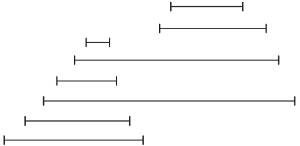
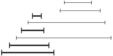
We now prove that it is possible to transform Algorithm A into an online version, Algorithm B, which is listed in Fig. 4.
Lemma 1.
Algorithm B is an online algorithm for the h-OVERLAP-COLORING problem producing a coloring identical to the coloring produced by Algorithm A. Algorithm B processes one interval in time.
Proof.
Let be a permutation of the integers from to such that for . Now we consider the sequence where the ’th number is . There is a simple one-to-one correspondence between a decreasing subsequence of this sequence and a chain of intervals from the set : If we start at the bottom of a chain and move upward, then the -values increase and the -values decrease. This means that we obtain a partition of into a minimum number of chains, if we apply the Patience Sorting method described in Section 2.2 and partition the sequence into a minimum number of decreasing subsequences.
Algorithm B processes the intervals in increasing order of their starting points applying the Patience Sorting method, and decisions on an interval are made without considering intervals with bigger starting points. The same goes for the splitting into smaller chains as well as the coloring of the chain bottoms and the other intervals. This means that Algorithm B is an online algorithm producing the same coloring as Algorithm A.
Each step of the Patience Sorting method requires time if we use binary search to locate the right pile. Keeping track of unused colors can also be handled in time for each step if a priority queue is used (a priority queue storing information on when the colors expire is used for the set in Fig. 4). ∎
Algorithm B(, ): Assumption on : 1: 2: 3: 4: for do 5: false 6: Let be the set of chains in where the top of the chain contains . 7: if then 8: Add a new chain to consisting of . 9: true 10: else 11: Let be the chain in with a top interval with the smallest value of . 12: Put on top of . 13: Let be the color assigned to . 14: if there are less than intervals in with color then 15: Assign color to . 16: else 17: true 18: end if 19: end if 20: 21: if true then 22: Let 23: if then 24: 25: Assign color to . 26: 27: else 28: Pick any . 29: Assign color to . 30: 31: end if 32: end if 33: end for
4 Probabilistic Analysis
Let be the clique number of the interval graph formed by the set of intervals . We remind the reader that is the minimum number of chains formed in step of Algorithm A.
Lemma 2.
The coloring produced by Algorithm A and B uses colors satisfying
| (4) |
Proof.
For any real number , we let denote the number of intervals in that contain and denote the number of chain bottoms produced in step of Algorithm A containing . As mentioned in Section 2.1, any interval graph can be colored with a number of colors corresponding to the size of the largest clique of the graph:
| (5) |
Now consider an interval that is a bottom of a chain produced in step of Algorithm A but not a bottom of one of the chains produced in step . If such an interval contains a number , then the intervals directly below it in the chain will also contain . There are at least such intervals that contain so we obtain the following inequality:
| (6) |
We now rearrange this inequality:
| (7) |
Next, we use (5) and . ∎
Our aim is to show that the competitive ratio of Algorithm B is close to with high probability. Formally, we say that an event occurs with high probability, abbreviated whp, if for . There is a number contained in intervals implying . Using Lemma 2, we can conclude that the competitive ratio is not bigger than . We will now show that the competitive ratio is whp. The strategy of our proof is to show that whp and that whp, and then combine these results.
For a brief moment, we leave the unknown distribution model and present a lemma for a simpler model for generating the instances: the uniform model. This model is obtained by substituting the unknown distribution in the unknown distribution model (see Definition 1) with the uniform distribution on . This is the only place in the paper where we are not using the unknown distribution model.
Lemma 3.
For the uniform model, the set of intervals can be partitioned into chains such that
Proof.
Let denote the ’th pair drawn using the uniform model. We introduce a permutation on the integers from to defined by for . We now look at the sequence of -values with as the ’th number in the sequence. We use the Patience Sorting method from Section 2.2 on the -sequence and obtain decreasing subsequences. We split each subsequence into two decreasing subsequences if there is a point where the -values become lower than their corresponding -values. It is not hard to see that we can form a chain of intervals for each of the up to subsequences we obtain by the splitting procedure (see Fig. 5).
Since , we have the following:
| (8) |
The - and -values are independent for the uniform model, so and have the same distribution, where is the length of the longest increasing subsequence for a permutation of numbers chosen uniformly at random (see Section 2.2):
| (9) |
Using (2), we get the following:
| (10) |
From (3), we observe that for sufficiently big. By using Chebyshevs inequality [10], we now get the following for sufficiently big:
| (11) |
From (8), (9), (10), and (11), we now get the following for sufficiently big:
| (12) |
From (12), we conclude that whp. ∎
We now use this lemma for the uniform model to prove a similar lemma for the more generic unknown distribution model.
Lemma 4.
For the unknown distribution model, the set of intervals can be partitioned into chains such that
Proof.
Without loss of generality, we assume that the unknown distribution has a density with with (we can always increase if necessarry). Let the function be defined as follows:
The function clearly qualifies as a probability density function. We now pick pairs independently by repeating the following procedure until pairs have been drawn using the -distribution:
- •
Pick a pair using with probability or with probability .
Let denote the total number of pairs picked by the procedure. Each time we pick a pair , we use a mixture of the distributions and : . This means that the pairs are picked using the uniform model described above. Let denote the minimum number of chains that we can form for the pairs we have picked using both distributions. Using Lemma 3, we conclude that whp. If we remove an interval from a chain, the chain is still a chain. This means that it is easy to transform a set of chains for the points picked by both distributions into a set of chains for the pairs of endpoints picked using the -distribution by deleting intervals picked using the -distribution: . Using the weak law of large numbers, we have whp implying whp. Finally, we get
| (13) |
∎
As a side remark, it should be noted that we could replace in (13) with any number strictly greater than . This shows that the upper bound matches and extends the result for the uniform distribution () from Lemma 3.
To illustrate a case where the premises of Lemma 4 are not satisfied, we can pick a number uniformly at random from and form the interval . In this case, we are not using the unknown distribution model for picking the endpoints from (there is a set with measure that has probability ). It is easy to see that with probability in this case. Ironically, our algorithm works perfectly when intervals are picked using this stochastic process.
Lemma 5.
For the unknown distribution model, we have the following:
Proof.
The triangle above the diagonal in the square can be partitioned into squares as illustrated in Fig. 6. The triangle below the diagonal can be partitioned in a similar way using squares .

We now have the following:
There must be at least one , , such that
and we also have the following for all :
According to the weak law of large numbers, will be contained in intervals whp. ∎
We now present a proof of the main theorem of the paper:
Proof (Theorem 1).
A corollary of Theorem 1 is that converges to in probability if . It is not hard to prove that , which implies , so as another corollary, the expected value of converges to if is a constant.
5 Experiments
We have performed some experiments to verify the theoretical results and to examine the underlying constants for the big O notation. For the first type of experiments, we have used the unknown distribution model introduced in Definition 1 with a uniform distribution on for some number as the ”unknown” distribution. In other words, we are choosing an interval with length up to uniformly at random. We use the notation for this type of experiment.
For the second type of experiments, we go beyond the unknown distribution model and choose the center and the length of an interval independently using two normal (Gaussian) distributions (if the length is negative, then we ignore it and pick a new length). This means that any real number can be an interval endpoint. The notation is used for the second type of experiments, where and are the mean and the standard deviation for the center of an interval, and and are the corresponding entities for the length of an interval. We go beyond the unknown distribution model to look into an even broader setting.
The eight distributions that we have used are , , and , .
The stack capacity has been fixed to for all the experiments. The experiments examine three perspectives corresponding to the three subsections in this section. For every combination of the eight distributions and three perspectives, we have generated random instances: one instance for each in the set . Please note that no instances have been reused.
5.1 Experiments for the Number of Chains
Lemma 4 is a key lemma specifying an upper bound on , i.e., the minimum number of chains that can be formed for an instance of the stacking problem. The values of have been plotted against in Fig. 7 and Fig. 8 for the uniform type and the Gaussian type of distributions, respectively.

The experiments clearly verify Lemma 4 by showing that – even when we go beyond our unknown distribution model using the Gaussian distributions. The underlying constant seems to be moderate, and holds for all the instances with depending on the actual distribution.
5.2 Convergence Rate Experiments
We now take a closer experimental look at our main contribution: Theorem 1. Our purpose is to verify the theorem and examine the actual convergence rate for the eight distributions that we consider. Directly inspired by our theorem, we have plotted against in Fig. 9 and Fig. 10. We remind the reader that so is an upper bound on the competitive ratio that we can efficiently compute (as mentioned earlier, we have no efficient procedure for computing for at the moment).

Similar to the experiments with the number of chains , we conclude that with an underlying moderate constant . From the graphs, we can se that is satisfied for all our instances.
5.3 Competitive Ratio Experiments
For the sake of completeness, we ran some experiments and plotted the upper bound for the competitive ratio, , against . The results are shown in Fig. 11 and Fig. 12.

These graphs confirm that the competitive ratio converges to in probability.
Conclusion
We have presented a simple polynomial time online algorithm for stacking with a competitive ratio that converges to in probability under the unknown distribution model. The main message of our paper is that such an algorithm exists. The experimental part of our paper shows that the results also have practical relevance. We do not think that our algorithm is better than similar algorithms presented in the literature, and we strongly believe that there are other asymptotically optimal algorithms for online stacking.
References
- [1] David Aldous and Persi Diaconis. Longest increasing subsequences: From patience sorting to the baik-deift-johansson theorem. Bull. Amer. Math. Soc, 36:413–432, 1999.
- [2] Mordecai Avriel, Michal Penn, and Naomi Shpirer. Container ship stowage problem: complexity and connection to the coloring of circle graphs. Discrete Applied Mathematics, 103(1-3):271 – 279, 2000.
- [3] Bram Borgman, Eelco van Asperen, and Rommert Dekker. Online rules for container stacking. OR Spectrum, 32(3):687–716, 2010.
- [4] Sabine Cornelsen and Gabriele Di Stefano. Track assignment. Journal of Discrete Algorithms, 5(2):250 – 261, 2007.
- [5] Marc Demange and Martin Olsen. A note on online colouring problems in overlap graphs and their complements. In WALCOM 2018, volume 10755 of Lecture Notes in Computer Science, pages 144–155. Springer, 2018.
- [6] Marc Demange, Gabriele Di Stefano, and Benjamin Leroy-Beaulieu. On the online track assignment problem. Discrete Applied Mathematics, 160(7-8):1072–1093, 2012.
- [7] Mark B. Duinkerken, Joseph J. M. Evers, and Jaap A. Ottjes. A simulation model for integrating quay transport and stacking policies on automated container terminals. In Proceedings of the 15th European Simulation Multiconference (ESM2001), 2001.
- [8] Saif Eddine Hamdi, Akram Mabrouk, and Thomas Bourdeaud’Huy. A heuristic for the container stacking problem in automated maritime ports. IFAC Proceedings Volumes, 45(6):357 – 363, 2012.
- [9] Klaus Jansen. The mutual exclusion scheduling problem for permutation and comparability graphs. Information and Computation, 180(2):71 – 81, 2003.
- [10] Hisashi Kobayashi, Brian L. Mark, and William Turin. Probability, Random Processes, and Statistical Analysis: Applications to Communications, Signal Processing, Queueing Theory and Mathematical Finance. Cambridge University Press, 2012.
- [11] Felix G. König, Marco E. Lübbecke, Rolf H. Möhring, Guido Schäfer, and Ines Spenke. Solutions to real-world instances of pspace-complete stacking. In Algorithms - ESA 2007: 15th Annual European Symposium, volume 4698 of Lecture Notes in Computer Science, pages 729–740. Springer, 2007.
- [12] Martin Olsen and Allan Gross. Probabilistic analysis of online stacking algorithms. In Computational Logistics - 6th International Conference, ICCL 2015, volume 9335 of Lecture Notes in Computer Science, pages 358–369. Springer, 2015.
- [13] Dario Pacino and Rune Møller Jensen. Fast Generation of Container Vessel Stowage Plans: using mixed integer programming for optimal master planning and constraint based local search for slot planning. PhD thesis, IT University of Copenhagen, 2012.
- [14] Shaiy Pilpel. Descending subsequences of random permutations. Journal of Combinatorial Theory, Series A, 53(1):96 – 116, 1990.
- [15] Rui Jorge Rei and João Pedro Pedroso. Tree search for the stacking problem. Annals OR, 203(1):371–388, 2013.
- [16] Kevin Tierney, Dario Pacino, and Rune Møller Jensen. On the complexity of container stowage planning problems. Discrete Applied Mathematics, 169(0):225 – 230, 2014.
- [17] Ning Wang, Zizhen Zhang, and Andrew Lim. The stowage stack minimization problem with zero rehandle constraint. In IEA/AIE (2), volume 8482 of Lecture Notes in Computer Science, pages 456–465. Springer, 2014.