Off-Policy Risk-Sensitive Reinforcement Learning Based Constrained Robust Optimal Control
Abstract
This paper proposes an off-policy risk-sensitive reinforcement learning based control framework for stabilization of a continuous-time nonlinear system that subjects to additive disturbances, input saturation, and state constraints. By introducing pseudo controls and risk-sensitive input and state penalty terms, the constrained robust stabilization problem of the original system is converted into an equivalent optimal control problem of an auxiliary system. Then, aiming at the transformed optimal control problem, we adopt adaptive dynamic programming (ADP) implemented as a single critic structure to get the approximate solution to the value function of the Hamilton-Jacobi-Bellman (HJB) equation, which results in the approximate optimal control policy that is able to satisfy both input and state constraints under disturbances. By replaying experience data to the off-policy weight update law of the critic artificial neural network, the weight convergence is guaranteed. Moreover, to get experience data to achieve a sufficient excitation required for the weight convergence, online and offline algorithms are developed to serve as principled ways to record informative experience data. The equivalence proof demonstrates that the optimal control strategy of the auxiliary system robustly stabilizes the original system without violating input and state constraints. The proofs of system stability and weight convergence are provided. Simulation results reveal the validity of the proposed control framework.
Keywords: Off-policy risk-sensitive reinforcement learning, adaptive dynamic programming, robust control, state constraint, input saturation.
I Introduction
Recently adaptive dynamic programming (ADP), which emerges as a successful implementation of reinforcement learning (RL) in the control field, has been proposed to approximately solve regulation or tracking problems of continuous or discrete time nonlinear systems with performance and/or robustness requirements, see [1, 2], and the references therein. The artificial neural network (NN) based approximate solution to the value function of the Hamilton-Jacobi-Bellman (HJB) equation facilitates the approximate optimal control strategy under an actor-critic structure. However, although traditional ADP has been widely adopted to tackle performance and robustness problems, input and state constraint satisfaction during the learning process, which is mainly investigated for safety concerns (e.g, restrictions on torques, joint angels and angular velocities of robot manipulators), has not yet been efficiently addressed. Violations of any of them could lead to possible serious consequences such as damage to physical components. This motivates us to develop a constraint-satisfying ADP-based control strategy. Furthermore, for practical applications, the constraint-satisfying control strategy should guarantee desired performance even under an uncertain environment.
I-A Prior and related works
Constrained ADP: In previous ADP related works [3, 4], by incorporating a suitable nonquadratic functional into the cost function, control limits have been addressed under an actor-critic structure, which leads to a bounded approximate optimal control policy in the form of a bounded hyperbolic tangent function. However, comparing with traditional ADP where a quadratic functional is usually adopted to represent the desired performance regarding control efforts [5], the introduced nonquadratic functional leads to an inevitable performance compromise problem that is ignored in existing related works [3, 4]. In terms of restrictions on system states, most of previous ADP related works adopt the system transformation technique to deal with state constraints under an actor-critic structure [6, 7, 8]. This method seeks for appropriate variable transformations that enable transformed system states to approach to infinity when potential state constraint violation happens. Therefore, approximate optimal control strategies that could achieve bounded transformed system states are constraint-satisfying control policies of the original system. The system transformation technique, nonetheless, is limited to simple constraint forms, e.g., restricted working space in a rectangular form. For certain state constraints, it may be infeasible to find suitable variable transformations to convert the constrained problem into an unconstrained counterpart. Besides, although general state constraints could be tackled by the well-designed penalty functions [4, 9], which become dominant in the optimization process when possible constraint violation happens and thus punish potential dangerous behaviours, no strict constraint satisfaction proofs are provided. However, in certain cases such as human-robot interaction, even the violation of constraints regarding safety issues in a small possibility is not allowed. Moreover, the trade-off between constraint satisfaction and performance is ignored in [4, 9], wherein control strategies that partially focus on constraint satisfaction or performance often result in a lack of practicability [10].
Single critic structure: For actor-critic structure adopted in the aforementioned ADP related works, the interplay between actor and critic NN is likely to cause instability because a wrong step taken by either of an actor or critic learning agent might adversely affect the other and destabilize the learning process [11]. To solve this potential instability problem, a single critic structure is adopted in [12] where the approximated value function from the critic NN is directly used to construct the approximate optimal control policy. The prerequisite of straightly using the approximated value function to construct the control policy is that the weight convergence of the estimated critic NN to the actual value is guaranteed. However, to the best of our knowledge, no strict proofs and/or simulation results have been provided to declare the guaranteed weight convergence to the actual value in most of single critic structure related works [12, 13, 14]. Conventionally, the weight convergence is checked by the persistence of excitation (PE) condition [15]. Among existing ADP related works [5, 16], the PE condition has been satisfied by directly adding external noises to inputs to achieve a sufficient exploration of the operation space. However, this method is unfavorable to practical applications given that the direct incorporation of external noises into control inputs may degrade control performance and cause nuisance, waste of energy, etc. Furthermore, in this method, the choice of explicit noise forms and the time to remove them during the online learning process highly depend on prior knowledge. Hence, for the guaranteed weight convergence, a more practical and easily implemented method to satisfy the PE condition is needed.
Experience replay: Given the fact that the satisfaction of the PE condition implies that available data regarding unknown weights to be learned are rich enough during the entire learning period [17], a feasible way to get the desired rich data is to reuse past data generated during the learning process. Recently experience replay (ER) emerges as an effective data-generating mechanism that replays experience data to accelerate the online learning process [18]. In ADP related works [6, 19], a fixed number of recently recorded transitions are replayed to actor or critic learning agents to avoid the necessity of using external noises to satisfy the required PE condition for the weight convergence. However, for this sequent way of data usage, experience data with different richness levels are used without discrimination, and partial informative data (e.g., data from initial exploring phases) are only used once then abandoned immediately. These characteristics of data usage result in poor sample efficiency and the collected data might not be rich enough for the weight convergence. Such a sample deficiency problem also exists in uniform sampling based ER techniques where all transitions are replayed at a same frequency regardless of their significance [20]. Unlike replaying experience data in a sequent or an uniform sampling way, prioritized experience replay (PER) is a more efficient technique that prioritizes data according to certain criteria [21]. Although all the aforementioned ER techniques have shown promise to accelerate learning, the implementation often accompanies with prior experience and extensive parameter tuning [6, 19]. To the best of our knowledge, there exists no related works on principled ways to provide rich enough experience data to accelerate the online leaning process.
I-B Contribution
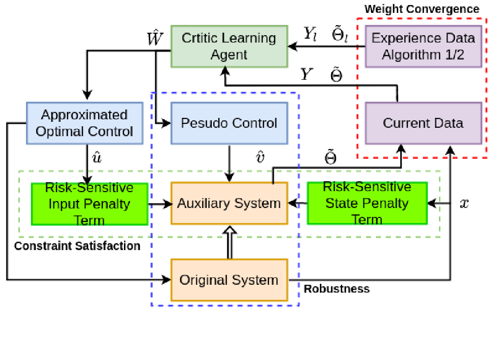
This work focuses on an off-policy risk-sensitive RL-based control framework, as summarized in Fig.1, for the control task of a nonlinear system under additive disturbances, input and state constraints. Based on pseudo controls, risk-sensitive input and state penalty terms, we transform a generally intractable constrained robust stabilization problem into an optimal control problem, which is then approximately solved by ADP under a single critic structure with an off-policy weight update law. The contribution of this paper is three-fold. First, we propose novel risk-sensitive state penalty terms to act as risk criteria during the learning process, which enables us to tackle state constraints in a long time-horizon, and preserve performance with strict constraint satisfaction proofs. Second, by exploiting experience data, we design an efficient off-policy critic NN weight update law that guarantees weight convergence without causing undesirable oscillations and additional control effort expenditures. Third, principled ways implemented as online and offline experience buffer construction algorithms are proposed to provide the required rich enough experience data for the weight convergence.
The remainder of this article is organized as follows. Section II provides the formulation of a constrained robust stabilization problem, the transformation to an optimal control problem, and the problem equivalence proof. Section III elucidates the approximated solution to the optimal control problem and the off-policy weight update law. Besides, the critic NN weight convergence proof and the system stability proof are provided. Simulation results shown in Section IV illustrate the effectiveness of the proposed control framework. Finally, Section V concludes this paper.
Notations: Throughout this paper, () denotes the set of real (positive) numbers; denotes the set of positive natural numbers; is the Euclidean space of -dimensional real vector; is the Euclidean space of real matrices; represents the identity matrix with dimension ; and denote the interior and boundary of the set , respectively; and are the maximum and minimum eigenvalues of a symmetric matrix , respectively; is the diagonal matrix with the value of main diagonal as ; The -th entry of a vector is denoted by , and is the Euclidean norm of the vector ; The -th entry of a matrix is denoted by , and is the Frobenius norm of the matrix . For notational brevity, time-dependence is suppressed without causing ambiguity.
II Problem formulation
II-A Formulation of constrained robust stabilization problem
Consider the continuous-time nonlinear dynamical system:
| (1) |
where and are states and inputs of the system. , are the known drift and input dynamics, respectively. represents the known differential system function. denotes the unknown additive disturbance. The general case that the additive disturbance is unmatched, i.e., , is considered. Assuming that and , which means that the equilibrium point is .
Before proceeding, the following assumptions are provided, which are common in ADP related works.
Assumption 1.
[3] is Lipschitz continuous on a set that contains the origin, and the system is stabilizable on . There exists such that the input dynamics is bounded by .
Assumption 2.
[22] The unknown additive disturbance is bounded by a known nonnegative function : , and .
Based on the aforementioned settings, we formulate the constrained robust stabilization problem (CRSP) as follows.
Problem 1 (CRSP).
Given Assumptions 1-2, design a control strategy such that the closed-loop system (1) that subjects to additive disturbances is stable under input saturation
| (2) |
where is a known saturation bound; and state constraints
| (3) |
where is a closed and convex set that contains the origin in its interior; is a known continuous function that relates with the -th state constraint; is the number of considered state constraints.
II-B Transformation to optimal control problem
Problem 1 can be decomposed into three sub-problems: disturbance rejection, input saturation and state constraint. It is not trivial for ADP to directly deal with these sub-problems together [1]. Thus, in this section, with pseudo controls proposed in [22], reformulated risk-sensitive input penalty terms based on [3], and our newly designed risk-sensitive state penalty terms, we firstly transform the CRSP clarified as Problem 1 into an equivalent optimal control problem, and then attempt to solve the aforementioned sub-problems simultaneously under an optimization framework.
II-B1 Pseudo control and auxiliary system
To address the additive disturbance under an optimization framework, firstly, by following [22], we decompose as a sum of matched and unmatched disturbance elements
| (4) |
where , and denotes the Moore-Penrose inverse.
Assumption 3.
[22] The continuous function is bounded as ; is bounded by a nonnegative function : , and .
Then, a pseudo control is introduced here, which is used to tackle the unmatched disturbance in (4), and the resulting auxiliary system follows [22]
| (5) |
By focusing on the auxiliary system (5) and incorporating the squared matched/unmatched disturbance bound (i.e, and ) into the cost function (6), we can address the additive disturbance under an optimization framework. The corresponding proofs are provided later in Theorem 1.
II-B2 Risk-sensitive input and state penalty terms
To tackle input/state constraints under an optimization framework, here we follow the idea of risk-sensitive RL where multiple risk measures, e.g, high moment or conditional value at risk, are used to deal with constraints of Markov decision processes [23]. However, the available risk measures in the risk-sensitive RL field cannot guarantee strict constraint satisfaction and/or not efficient (even inappropriate) to address constraints of continuous nonlinear systems. Thus, we propose risk-sensitive input penalty term (RS-IP) in Definition 1 and risk-sensitive state penalty term (RS-SP) in Definition 2 as new risk measures during the learning process to enforce strict satisfaction of input/state constraints of continuous nonlinear systems.
Definition 1 (RS-IP).
A continuous and differential function is a risk-sensitive input penalty term if it has the following properties:
(1) A bounded monotonic odd function with ;
(2) The first-order partial derivatives of is bounded.
Here the RS-IP term is a reformulation of the nonquadratic functional used in [3, 12] to confront input constraints.
Definition 2 (RS-SP).
Given the closed region , , defined as (3), a continuous scalar function , , is a risk-sensitive state penalty term if the following proprieties hold:
(1) , and ;
(2) if approaches ;
(3) For initial value , there exists such that along solutions of the dynamics.
Comparing with similar works [4, 9] that use state penalty functions to tackle state constraints but without strict constraint satisfaction proofs, the proposed RS-SP term enables us to provide strict constraint satisfaction proofs in Theorem 1. Here the novel RS-SP term is inspired by the so-called barrier Lyapunov function [24]. The first point of Definition 2 denotes that is an effective Lyapunov function candidate, which enables to serve as part of Lyapunov function for the system stability proof. The last two points imply that and , which means that serves as a barrier certificate for an allowable operating region .
II-B3 Optimal control problem
Based on the auxiliary system (5) and Definitions 1-2, an equivalent optimal control problem (OCP) of CRSP in Problem 1 is clarified as Problem 2. Comparing with traditional ADP that accomplishes partial objectives of performance, robustness, and input/state constraint satisfaction [1, 2, 3, 4], the applied problem transformation here enables us to consider such multiple objectives together.
Problem 2 (OCP).
Given Assumptions 1-3, consider the auxiliary system (5), find and to minimize the cost function
| (6) |
where the utility function with , , and . The input penalty function is defined as
| (7) |
where is the RS-IP term in Definition 1; is the -th diagonal element of a positive definite diagonal matrix . The state penalty function is defined as
| (8) |
where is a positive definite matrix; is the risk sensitivity parameter that follows , where is the distance from the state to the boundary of ; is the RS-SP term in Definition 2 for -th state constraint.
Unlike ADP related works [3, 4] that incorporate nonquadratic functionals to tackle input saturation but without considering performance regarding control efforts, by choosing suitable matrix , in (7) could take into consideration of requirements for both control limits and control energy expenditures. Much more details are introduced in Section II-C1. The common used risk-neutral quadratic function [1, 2] (capturing the desired state performance) is augmented with the newly designed weighted RS-SP term (addressing multiple state constraints) to construct in (8), which enables us to consider state-related performance and constraint satisfaction together. The incorporation of into deteriorates the desired performance represented by . Therefore, we propose the risk sensitivity parameter , which relates with the distance from the constraint boundary, to specify the inevitable trade-off between the state-related performance and constraint satisfaction during the learning process. Note that this kind of trade-off is ignored in existing related works [4, 9]. The detailed mechanism of is illustrated in Section II-C2.
II-C Mechanism of input and state penalty functions
The mechanism of and to enable the learning process to preserve performance without violating strict input/state constraint satisfaction is clarified here.
II-C1 Mechanism of input penalty function
By Definition 1, the explicit form of the RS-IP term is chosen as [3]. Given the inevitable trade-off between constraint satisfaction and performance regarding control inputs, are designed to counter input constraints (2) and approximate (a common desired performance criterion for control efforts) simultaneously, where is a positive definite matrix designed according to users’ preferences.


The mechanism of to tackle input constraints can be clarified from two perspectives, see Fig.2(a) and Fig.2(b), respectively. In the first perspective, input constraints are considered in a long time-horizon. in (7) is an integration of that is denoted as in Fig.2(a). When any , , approaches to the input constraint boundaries , it follows that the value of will be infinity. Since the optimization process aims to minimize the cost function, the resulting optimal control strategy will be away from ; Otherwise, a high value of the cost function occurs. From the other perspective, according to the later result in (12), the resulting optimal control strategy based on is in a form of whose boundness enforces strict satisfaction of input constraints, as shown in Fig.2(b). The construction of to reflect the desired performance for control energy is shown in Fig.2(c). Consider , the -th summand of . It follows that
| (9) |
As displayed in Fig.2(c), by adjusting the value of , can approximate the desired control energy criterion well. Based on the above discussion, we know that in (7) can tackle input constraints while preserving performance concerning control energy expenditures.
II-C2 Mechanism of state penalty function
According to Definition 2, when a potential state constraint violation happens, the corresponding RS-SP term will approach to infinity. Since the optimal control strategy aims to minimize the total cost, states will be pushed away from the direction where a high value of the RS-SP based occurs. Thus, the state constraint violation is avoided. To satisfy Definition 2, we choose here. Note that the explicit form of is adjusted based on given state constraints, which is exemplified later. For a better explanation of the mechanism of the RS-SP term and the corresponding risk sensitivity parameter , we present a four-dimensional system example with safe region defined as [25], , and [6]. The corresponding RS-SP terms are designed as with , , and , respectively. As displayed in Fig.3(a)-3(b), these RS-SP terms act as barriers at constraint boundaries and confine states remain in the safe regions. This inherent risk-sensitive property enables us to tackle state constraints under an optimization framework. As long as initial states lie in the safe regions and the cost function is always bounded as time evolves, the subsequent state evolution will be restricted to the safe regions. From Fig.3(c)-3(d), we know that the role of will be discouraged by when states are far away from the boundary of . Therefore, performance regrading states is maintained when no state constraint violation occurs.


II-D HJB equation for the OCP
II-E Equivalence between Problem 1 and Problem 2
Here we defer a detailed explanation of the method to get the optimal control policies (12) and (13) in Section III, and focus now on the proof of equivalence between Problem 1 in Section II-A and Problem 2 in Section II-B. Comparing with the result provided in [22] that merely considers additive disturbances, as shown in Theorem 1, the additional consideration of input and state constraints further complicates the theoretical analysis.
Theorem 1.
Consider the system described by (1) and controlled by the optimal control policy (12). Suppose Assumptions 1-3 hold and the initial states and control inputs lie in the predefined constraint satisfying sets (2) and (3). The optimal control policy (12) guarantees robust stabilization of the system (1) without violating input constraint (2) and state constraint (3), if there exists a scalar such that the following inequality is satisfied
| (14) |
Proof.
See Appendix A. ∎
III Approximate solutions to the OCP
To get approximated solutions to the OCP, instead of introducing a common actor-critic structure used in [3, 5], here we adopt a single critic structure which enjoys lower computation complexity [14]. Furthermore, unlike common methods that add external noises into inputs to satisfy the required PE condition for the critic NN weight convergence [5, 16], here we exploit experience data to construct the off-policy weight update law to achieve a sufficient excitation required for the critic NN weight convergence. Additionally, an online PER algorithm and an offline experience buffer construction algorithm are proposed as principled ways to provide the aforementioned rich enough experience data.
III-A Value function approximation
According to the Weierstrass high-order approximation theorem [26], there exists a weighting matrix such that the value function is approximated as
| (15) |
where is the NN activation function, and is the approximation error. is the number of NN activation functions. The derivative of follows
| (16) |
where and are partial derivatives of and , respectively. As , both and converge to zero uniformly. Without loss of generality, the following assumption is given.
Assumption 4.
[5] There exist known constants such that , , and .
For fixed admissible control policies and , inserting (16) into (11) yields the Lyapunov equation (LE)
| (17) |
where the residual error follows . According to Assumption 1, the system dynamics is Lipschitz. This leads to the boundness of the residual error, i.e., there exists a positive scalar such that .
By focusing on the NN parameterized LE (17), unlike the common analysis and derivation process in typical ADP related works [1, 2], here we rewrite (17) into a linear in parameter (LIP) form that follows
| (18) |
where , and . Note that both and can be obtained from real-time data.
Given the LIP form and the measurable , in (18), from the perspective of adaptive control, we transform the learning of critic NN weight into a parameter estimation problem of an LIP system, where and can be treated as the regressor matrix and the unknown parameter vector of a LIP system, respectively. This novel transformation enables us to design a simple weight update law with weight convergence guarantee in Section III-B.
III-B Off-policy weight update law
The ideal critic weight in (18) is approximated by an estimated weight which satisfies the following relation
| (19) |
where is the estimated utility function. Denoting the weight estimation error as . Then, we can get
| (20) |
To achieve and , should be updated to minimize . Furthermore, in order to guarantee the weight convergence while minimizing , rather than incorporating external noises to satisfy the PE condition [5, 16], here we exploit experience data to accelerate the online learning process, which could achieve the sufficient excitation required for the weight convergence. Finally, we design a simple yet efficient off-policy weight update law of the critic NN that follows
| (21) |
where is a constant positive definite gain matrix. are constant gains to balance the relative importance between current and experience data to the online learning process. is the volume of the experience buffers and , i.e., the maximum number of recorded data points. The regressor matrix and the approximation error denote the -th collected data of the corresponding experience buffers and , respectively. The developed critic NN weight update law (21) is in a different form comparing with the counterpart in typical ADP related works (See [1, 2, 5] and the references therein). Our proposed weight update law (21) is easily implemented and enjoys guaranteed weight convergence without causing undesirable oscillations and additional control effort expenditures.
To analyse the weight convergence of the critic NN, a rank condition about the experience buffer , which serves as a richness criterion of the recorded experience data, is firstly clarified here in Assumption 5.
Assumption 5.
Given an experience buffer , there holds .
Comparing with the traditional PE condition given in [27], the rank condition regarding in Assumption 5 provides an index about the data richness that can be checked online, which is favourable to controller designers.
Based on the aforementioned settings, the critic NN weight convergence proof is shown as follows.
Theorem 2.
Given Assumption 5, the weight learning error converge to a small neighbourhood around zero.
Proof.
Consider the following candidate Lyapunov function
| (22) |
The time derivative of reads
| (23) | ||||
where , and . The boundness of and results in bounded , i.e., there exists such that . Since is positive definite according to Assumption 5, (23) can be written as
| (24) |
Therefore, if . Finally, it is concluded that the weight estimation error of the critic NN will converge to the residual set defined as
| (25) |
This completes the proof. ∎
By observing (25), the size of relates with the bound of . As , we know that results in . Then, we get , i.e., exponentially as . Equivalently, it is guaranteed that converges to . Finally, in conjugation with (12) and (13), the approximate optimal control policies are obtained as
| (26) |
| (27) |
In the following part, the main conclusions are provided based on the off-policy weight update law (21) and the approximate optimal control policies (26), (27).
Theorem 3.
Consider the dynamics (5), the off-policy weight update law of the critic NN in (21), and the control policies (26) and (27). Given Assumptions 1-5, for sufficiently large , the approximate control policies (26) and (27) stabilize the system (5). Moreover, the critic NN weight learning error is uniformly ultimately bounded (UUB).
Proof.
See Appendix B. ∎
Assumption 5 in Theorem 3 is the prerequisite to ensure that converges to . The guaranteed weight convergence enables us to directly apply in (21) to construct the approximate optimal control policies (26), (27). Assumption 5 is not restrictive and can be easily satisfied by the algorithms proposed in the next section.
III-C Experience replay with online and offline experience buffers
To get rich enough experience data to satisfy Assumption 5, given the sampling deficiency problem of the subsequent way of data usage in existing ADP related works [6, 19], and inspired by the concurrent learning (CL) technique developed for system identification [28], here we design both online and offline principled methods to provide the required rich enough experience data to satisfy Assumption 5. To the best of our knowledge, this is the first attempt to design principled ways of replaying rich enough experience data to achieve the required exploration for the critic NN weight convergence.
III-C1 Online PER algorithm
Before the estimated weight converges (line 4-5), Algorithm 1 chooses the minimum eigenvalue (i.e., ) as the priority scheme to filter experience data , recorded into the experience buffers and , respectively. Here the prioritized criterion is different from ones used in existing PER algorithms [21]. We prefer experience data accompanied with a larger given the facts that: a) a nonzero ensures that in Assumption 5 holds [28], i.e., the convergence of to is guaranteed; b) according to (24) and (25), a larger leads to a faster weight convergence rate and a smaller residual set. Although efficient, the priority scheme accompanies with additional computation loads. Thus, on convergence (line 6-7), i.e., we have gotten sufficient excitation required for the weight convergence, we alternate to a low-cost way where recent experience data are sequentially recorded. This sequent way of data usage enjoys robustness to a dynamic environment since collected real-time data could reflect environmental changes in time. Unlike standard methods that first construct a huge experience buffer and then sample partial data [20], to reduce computation loads and relieve hardware requirements, we directly build experience buffers with a limited buffer size here, and all of the recorded experience data are replayed to the critic NN for the online weight learning. The buffer size is a hyper-parameter that requires careful tuning. In order to satisfy Assumption 5, is selected such that holds.
III-C2 Offline experience buffer construction algorithm
In addition to experience buffers and constructed from online data featured with sufficient richness and high minimum eigenvalues, in Algorithm 2, we construct experience buffers with offline collected experience data. Here the offline experience data are generated from the pre-simulation within the given operation region . To generate rich enough training data, for -th dimension of an allowable operation region , we can sample training data equidistantly with a fixed mesh size , or a predefined number . Besides, rather than sampling partial data from the offline constructed experience buffers based on an uniform or a prioritized way [20], we replay all offline experience data in an average way for the weight estimation. Thereby, the off-policy weight update law (21) based on Algorithm 2 is redesigned as
| (28) |
The implementation of using offline recorded experience data to accelerate the online learning process enjoys two advantages: the rank condition in Assumption 5 is easily satisfied, and the possible influence of data noises is offset by averaging.
Remark 1.
The subsequent [6, 19] or uniform sampling way [20] of data usage cannot ensure that Assumption 5 is always satisfied, whereas, the developed online PER algorithm not only guarantees establishment of Assumption 5, but also accelerates the weight convergence speed. Besides, in the CL algorithm [28], a constant hyperparameter that highly depend on prior knowledge is required to characterize the data richness, which results in additional parameter tuning effort. This is avoided in Algorithm 1 by calculating the rank value of the experience buffer , even though additional (but acceptable) computation load is unintentionally introduced.
Remark 2.
The simple three-layer NNs adopted in this paper provides us with opportunities to revisit the ER technique and investigate principled ways to exploit experience data to accelerate the online learning process, which is difficult in the deep RL field because the complexity of deep NNs hinders researchers from understanding the mechanism of the ER technique [20]. Algorithms 1-2 are plug-in methods, which can be widely used with little extra computations and engineering efforts. We argue that they also provide alternative solutions for the parameter convergence problem existing in the adaptive control field.
IV Numerical simulations
This section provides three simulation examples to show the effectiveness of the proposed off-policy weight update laws (21), (28), the approximate optimal control policy (26), and Algorithms 1-2. Firstly, we consider an optimal regulation problem (ORP) of a nonlinear system [5] in Section IV-A. This ORP serves as a benchmark problem to prove that both Algorithm 1 based (21) and Algorithm 2 based (28) enable the estimated critic NN weight to converge to the actual optimal value, which is marginally considered in existing single critic structure related works [12, 13]. Then, to show the superiority of our proposed off-policy risk-sensitive RL-based control framework to counter input and state constraints under additive disturbances, a pendulum system [29] is investigated in Section IV-B. Furthermore, a target (set-point) tracking control problem of a 2-DoF robot manipulator [30] is investigated in Section IV-C to validate the real-time performance of our proposed control framework.
IV-A Example 1: ORP of a benchmark nonlinear system
To validate that based on our proposed off-policy weight update laws (21), (28), and Algorithms 1-2, the estimated weight guarantees convergence to the actual optimal value, a benchmark problem [5] is investigated here. Note that only an optimal regulation problem without considering disturbances nor input/state constraints is investigated here. Otherwise, the actual optimal value of the NN weight is unknown. The benchmark continuous-time nonlinear system is given as
where , . The standard quadratic cost function follows
where and . By following the converse HJB approach developed in [31], we get the optimal value function as . Thus, by choosing the activation function as , the optimal weight follows . Initial values are set as , . For the off-policy weight update law (21) based on Algorithm 1, we choose , , , , and . It is displayed in Fig.4(a) that after s, the estimated weight converges to
Regarding the weight update law (28) under Algorithm 2, we start with constructing offline experience buffers by sampling data points separately for , . , , , and are chosen during the online operation. As displayed in Fig.4(b), the estimated weight converges to
Thus, it is concluded that the weight update laws (21), (28) under Algorithms 1-2 ensure that converges to . Comparing with the results shown in [5], without incorporating external noises to satisfy the PE condition, our proposed off-policy weight update laws enable converge to with a fast speed.


IV-B Example 2: CRSP of a pendulum system
This section investigates the CRSP (Problem 1) of a pendulum system to validate the effectiveness and efficiency of the proposed control framework shown in Fig.1. The state-space model of a pendulum system is given as [29]
where , , , and . During the simulation, and are randomly chosen within the scope and , respectively. Thus, and establishes, and Assumptions 2-3 can be satisfied by choosing and . Here the input and state constraints are considered as and , , where , , and . The corresponding auxiliary system follows
| (29) |
where . Let , , , and . For the CRSP of pendulum, the cost function of (29) follows
where , . For comparison, a robust optimization problem (ROP) for the pendulum without considering input and state constraints is also investigated here. Regarding the ROP case, the common quadratic cost function given in [32] is recalled here. By setting for the term and for the term, the cost function of (29) follows
The activation function for the pendulum is chosen as . For the off-policy weight update law (21) based on Algorithm 1, , , , , and are chosen. The initial valuesare set as , , , and . Note that the initial values of states are purposely set to be near the constraint boundaries to highlight the efficacy of our method. Simulation results for the pendulum system are shown as follows.


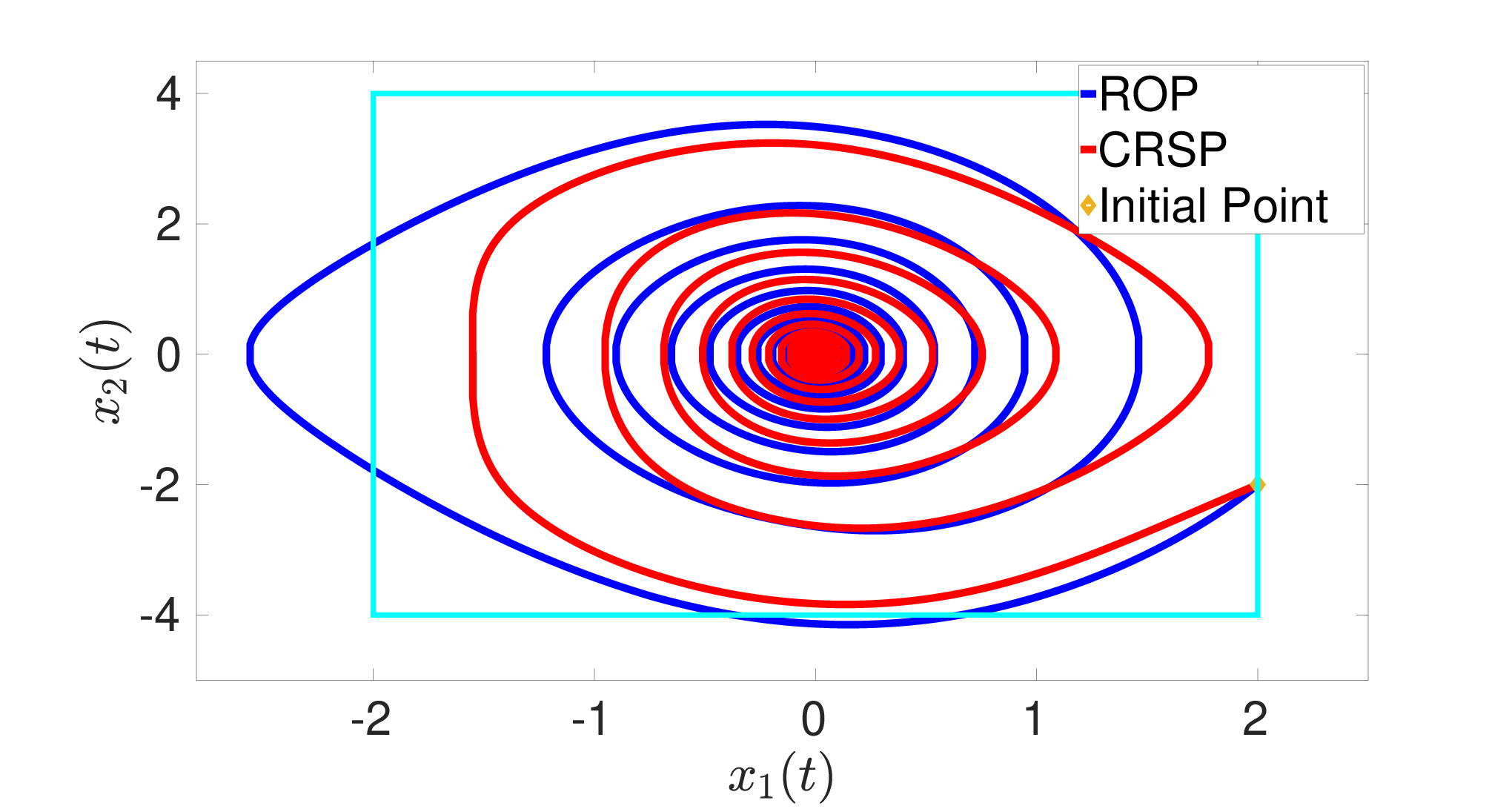
The evolution trajectory of the estimated critic NN weight of the CRSP case is shown in Fig.5(a). It is observed that after , the convergence result of achieves. As displayed in Fig.5(b), the control trajectory of the CRSP case illustrates that the RS-IP term enables the satisfaction of input constraints. However, for the ROP case, the input constraint boundary is violated. The phase portrait of states is provided in Fig.5(c) where the cyan rectangle represents the state constraint boundary. It is observed that states , asymptotically converge to the equilibrium point and always lie in the state constraint set for the CRSP case. However, for the ROP case, the predefined state constraint is violated. The simulation results displayed in Fig.5 have verified that the resulting approximate optimal control policy by solving Problem 2 can efficiently deal with Problem 1.
IV-C Example 3: CRSP of a 2-DoF Robot Manipulator
To further demonstrate the real-time performance of our proposed control framework, we consider a target (set-point) tracking control problem of a 2-DoF robot manipulator in this section. The objective is to drive the robot manipulator to reach the target point under additive disturbances, input and state constraints. For brevity, denoting , , , . Then, the Euler-Lagrange (E-L) equation of a 2-DoF robot manipulator follows [30]
where the inertia matrix is , and the matrix of centrifugal and Coriolis terms follows . Let , the above E-L equation can be written in the state-space form as (1), where , and . Besides, with , we assume that the robot manipulator suffers an additive disturbance that follows , where . Given , and , Assumptions 2-3 can be satisfied by setting , and . The input constraints are considered as , . The state constraint in a rectangular form has been considered in Section IV-B. Thus, to show the effectiveness of the proposed RS-SP term to deal with general state constraints, a circular state constraint is considered here. The solution procedure for the robot manipulator’s CRSP is similar to Section IV-B. Thus, the detailed explanation is omitted here for page limits. To fully demonstrate the effectiveness of our proposed control framework to address state constraints even under input saturation and environmental disturbances, the phase plot under multiple initial positions is shown in Fig.6, where the robot manipulator is driven to reach the target point (zero point) while obeying the predefined state constraints. We observe that when states approach to the constraint boundary, they will be driven back to safe states under the proposed control framework.

In this section, we choose the activation function as . The weight convergence result is displayed in Fig.7, where the weight convergence result under our proposed weight update law (21) achieves at . The aforementioned simulation results based on a 2-DoF robot manipulator validate that the off-policy weight update law (21) and the approximate optimal control policy (26) fulfill real-time requirements.

V Conclusion
An off-policy risk-sensitive RL-based control framework is proposed to stabilize a nonlinear system that subjects to additive disturbances, input and state constraints. Firstly, the introduced pseudo control and the resulting auxiliary system enable us to address additive disturbances under an optimization framework. Then, risk-sensitive input and state penalty terms are incorporated into the cost function as optimization criteria, which allows us to tackle both input and state constraints in a long time-horizon. This helps to avoid the abrupt changes of control inputs that are unfavourable for the online learning process. The transformed OCP is solved by a single critic structure based ADP with an off-policy weight update law. The adopted single critic structure leads to computation simplicity and eliminates approximation errors caused by an actor NN. Besides, the exploitation of experience data to guarantee the weight convergence enables the proposed control strategy be applicable to practical applications. Multiple comparison results shown in the simulation part illustrate the effectiveness of the proposed control framework.
Appendix A Proof of Theorem 1
Proof.
(i) Proof of stability. As for defined as (10), we know that when , , and for . Thus, it can serve as a Lyapunov function candidate for stability proofs. Taking time derivative of along the system (1) yields
| (30) | ||||
In light of (11), we can get
| (31) | ||||
From (12), we can get
| (32) |
Based on (13), the following equation establishes
| (33) |
Substituting (31), (32) and (33) into (30) yields
| (34) | ||||
By setting , we can get
| (35) | ||||
where . Based on the integral mean-value theorem, there exist a series of , such that
| (36) |
Bearing in mind the relation (32) and the fact , it follows that
| (37) | ||||
According to the definition of the admissible policy [3], is finite. Moreover, there exists such that . Based on Assumption 1, we can rewrite (37) as
| (38) |
where . Based on Assumption 2, the following equations establish
| (39) | ||||
and
| (40) | ||||
By substituting (35), (38), (39) and (40) into (34), we have
| (41) | ||||
where . Thus, establishes, if the condition (14) holds. It yields that the optimal control policy robustly stabilizes the system (1).
(ii) Proof of input and state constraint satisfaction. Denote the value of the Lyapunov function candidate at . According to the definition of admissible control policies, is a bounded function. If , establishes, which means that , . The boundness of implies that state constraints will not be violated; otherwise, according to Definition 2, if any state constraint violations happens. Since the hyperbolic tangent function satisfies , the optimal control policy in (12) follows , i.e., inputs are confined into the safety set (2). The proof provided here means that the optimal control policy for the system (1) guarantees satisfaction of both constraints in terms of system states and control inputs. ∎
Appendix B Proof of Theorem 3
Proof.
Consider the following candidate Lyapunov function
| (42) |
Taking time derivative of (42) along the system (5) yields
| (43) |
where and .
The first term follows
| (44) | ||||
According to (31), (32) and (33), (44) can be rewritten as
| (45) | ||||
Besides, we can get
| (46) | ||||
Based on (35)-(41), the following equation also establishes
| (47) | ||||
Substituting (47) into (45) yields
| (48) | ||||
As for in (48), according to (27),
| (49) | ||||
where .
As for in (48), according to (27),
| (50) | ||||
For simplicity, denote and , with . Based on (12) and (26), the Taylor series of follows
| (51) | ||||
where , is a higher order term of the Taylor series. By following [33, Lemma 1], the higher order term is bounded as
| (52) |
Using (12), (26) and (51), we get
| (53) | ||||
where , and assuming that it is bounded by .
Substituting (49), (50), (54) into (48) yields
| (55) | ||||
As for the second term , based on (21) and (23),
| (56) |
Finally, as for , substituting (55) and (56) into (43), based on the fact that , , , we can get
| (57) | ||||
where , and there exists such that ; is positive definite; , and .
Let the parameters be chosen such that . Since is positive definite, the above Lyapunov derivative is negative if
| (58) |
Thus, the critic weight learning error converges to the residual set defined as
| (59) |
∎
References
- [1] D. Liu, F. L. Lewis, and Q. Wei, “Editorial special issue on adaptive dynamic programming and reinforcement learning,” IEEE Transactions on Systems, Man, and Cybernetics: Systems, vol. 50, no. 11, pp. 3944–3947, 2020.
- [2] F. L. Lewis and D. Vrabie, “Reinforcement learning and adaptive dynamic programming for feedback control,” IEEE circuits and systems magazine, vol. 9, no. 3, pp. 32–50, 2009.
- [3] M. Abu-Khalaf and F. L. Lewis, “Nearly optimal control laws for nonlinear systems with saturating actuators using a neural network hjb approach,” Automatica, vol. 41, no. 5, pp. 779–791, 2005.
- [4] J. Na, B. Wang, G. Li, S. Zhan, and W. He, “Nonlinear constrained optimal control of wave energy converters with adaptive dynamic programming,” IEEE Transactions on Industrial Electronics, vol. 66, no. 10, pp. 7904–7915, 2018.
- [5] K. G. Vamvoudakis and F. L. Lewis, “Online actor–critic algorithm to solve the continuous-time infinite horizon optimal control problem,” Automatica, vol. 46, no. 5, pp. 878–888, 2010.
- [6] Y. Yang, D.-W. Ding, H. Xiong, Y. Yin, and D. C. Wunsch, “Online barrier-actor-critic learning for h- control with full-state constraints and input saturation,” Journal of the Franklin Institute, 2019.
- [7] M. He, “Data-driven approximated optimal control for chemical processes with state and input constraints,” Complexity, vol. 2019, 2019.
- [8] J. Sun and C. Liu, “Disturbance observer-based robust missile autopilot design with full-state constraints via adaptive dynamic programming,” Journal of the Franklin Institute, vol. 355, no. 5, pp. 2344–2368, 2018.
- [9] M. Abu-Khalaf, J. Huang, and F. L. Lewis, Nonlinear H2/H-Infinity Constrained Feedback Control: A Practical Design Approach Using Neural Networks. Springer Science & Business Media, 2006.
- [10] J.-J. E. Slotine, W. Li et al., Applied nonlinear control. Prentice hall Englewood Cliffs, NJ, 1991, vol. 199, no. 1.
- [11] S. Parisi, “Reinforcement learning with sparse and multiple rewards,” Ph.D. dissertation, Technische Universität, 2020.
- [12] A. Heydari and S. N. Balakrishnan, “Finite-horizon control-constrained nonlinear optimal control using single network adaptive critics,” IEEE Transactions on Neural Networks and Learning Systems, vol. 24, no. 1, pp. 145–157, 2012.
- [13] X. Yang and H. He, “Event-triggered robust stabilization of nonlinear input-constrained systems using single network adaptive critic designs,” IEEE Transactions on Systems, Man, and Cybernetics: Systems, 2018.
- [14] R. Padhi, N. Unnikrishnan, X. Wang, and S. Balakrishnan, “A single network adaptive critic (snac) architecture for optimal control synthesis for a class of nonlinear systems,” Neural Networks, vol. 19, no. 10, pp. 1648–1660, 2006.
- [15] S. Boyd and S. S. Sastry, “Necessary and sufficient conditions for parameter convergence in adaptive control,” Automatica, vol. 22, no. 6, pp. 629–639, 1986.
- [16] S. Bhasin, R. Kamalapurkar, M. Johnson, K. G. Vamvoudakis, F. L. Lewis, and W. E. Dixon, “A novel actor–critic–identifier architecture for approximate optimal control of uncertain nonlinear systems,” Automatica, vol. 49, no. 1, pp. 82–92, 2013.
- [17] P. A. Ioannou and J. Sun, Robust adaptive control. Courier Corporation, 2012.
- [18] L.-J. Lin, “Self-improving reactive agents based on reinforcement learning, planning and teaching,” Machine learning, vol. 8, no. 3-4, pp. 293–321, 1992.
- [19] R. Kamalapurkar, P. Walters, and W. E. Dixon, “Model-based reinforcement learning for approximate optimal regulation,” in Control of Complex Systems. Elsevier, 2016, pp. 247–273.
- [20] W. Fedus, P. Ramachandran, R. Agarwal, Y. Bengio, H. Larochelle, M. Rowland, and W. Dabney, “Revisiting fundamentals of experience replay,” arXiv preprint arXiv:2007.06700, 2020.
- [21] T. Schaul, J. Quan, I. Antonoglou, and D. Silver, “Prioritized experience replay,” arXiv preprint arXiv:1511.05952, 2015.
- [22] F. Lin and R. D. Brandt, “An optimal control approach to robust control of robot manipulators,” IEEE Transactions on robotics and automation, vol. 14, no. 1, pp. 69–77, 1998.
- [23] Y. Shen, W. Stannat, and K. Obermayer, “Risk-sensitive markov control processes,” SIAM Journal on Control and Optimization, vol. 51, no. 5, pp. 3652–3672, 2013.
- [24] K. P. Tee, S. S. Ge, and E. H. Tay, “Barrier lyapunov functions for the control of output-constrained nonlinear systems,” Automatica, vol. 45, no. 4, pp. 918–927, 2009.
- [25] L. Wang, E. A. Theodorou, and M. Egerstedt, “Safe learning of quadrotor dynamics using barrier certificates,” in 2018 IEEE International Conference on Robotics and Automation (ICRA). IEEE, 2018, pp. 2460–2465.
- [26] B. A. Finlayson, The method of weighted residuals and variational principles. SIAM, 2013, vol. 73.
- [27] G. Tao, Adaptive control design and analysis. John Wiley & Sons, 2003, vol. 37.
- [28] G. V. Chowdhary, “Concurrent learning for convergence in adaptive control without persistency of excitation,” 2010.
- [29] D. Liu and Q. Wei, “Policy iteration adaptive dynamic programming algorithm for discrete-time nonlinear systems,” IEEE Transactions on Neural Networks and Learning Systems, vol. 25, no. 3, pp. 621–634, 2013.
- [30] C. Li, F. Liu, Y. Wang, and M. Buss, “Concurrent learning-based adaptive control of an uncertain robot manipulator with guaranteed safety and performance,” IEEE Transactions on Systems, Man, and Cybernetics: Systems, 2021.
- [31] V. Nevistić and J. A. Primbs, “Constrained nonlinear optimal control: a converse hjb approach,” 1996.
- [32] F. Lin, R. D. Brandt, and J. Sun, “Robust control of nonlinear systems: Compensating for uncertainty,” International Journal of Control, vol. 56, no. 6, pp. 1453–1459, 1992.
- [33] X. Yang, D. Liu, H. Ma, and Y. Xu, “Online approximate solution of hji equation for unknown constrained-input nonlinear continuous-time systems,” Information Sciences, vol. 328, pp. 435–454, 2016.