Stochastic Gradient Descent for Semilinear Elliptic Equations with Uncertainties

Ting Wang Address: Physical Modeling & Simulation Branch, CISD, CCDC U.S. Army Research Laboratory Jaroslaw Knap Address: Physical Modeling & Simulation Branch, CISD, CCDC U.S. Army Research Laboratory

Abstract

Randomness is ubiquitous in modern engineering. The uncertainty is often modeled as random coefficients in the differential equations that describe the underlying physics. In this work, we describe a two-step framework for numerically solving semilinear elliptic partial differential equations with random coefficients: 1) reformulate the problem as a functional minimization problem based on the direct method of calculus of variation; 2) solve the minimization problem using the stochastic gradient descent method. We provide the convergence criterion for the resulted stochastic gradient descent algorithm and discuss some useful technique to overcome the issues of ill-conditioning and large variance. The accuracy and efficiency of the algorithm are demonstrated by numerical experiments.

Keywords:

Semilinear PDE, polynomial chaos, uncertainty quantification, stochastic gradient descent, variance reduction

1 Introduction

Many problems in science and engineering involve spatially varying input data. Often, the input data is subject to uncertainties due to inherent randomness. For example, the details of spatial variations of properties and structure of engineering materials are typically obscure, and randomness and uncertainty are fundamental features of these complex physical systems. Under these circumstances, traditional deterministic models are rarely capable of properly handling this randomness and yielding accurate predictions. Therefore, in order to furnish accurate predictions, randomness must be incorporated directly into the model and the propagation of the resulting uncertainty between its input and output must be quantified accordingly. A model, particularly important in many applications, consists of the random input data in the form of a random field and a partial differential equation (PDE). The specific model problem considered here is

\mathcal{L}(\kappa)(u)=0\quad\textrm{in}~D

(1)

where $\mathcal{L}$ is a nonlinear elliptic operator dependent on a random field $\kappa$ over a probability space $(\Omega,\mathcal{F},\mathbb{P})$ , and $u$ is a solution. Examples of (1) include, but are not limited to, flow of water through random porous medium and modeling of the mechanical response of materials with random microstructure.

Over the past few decades, the critical need to seek solutions of (1) has yielded a wealth of numerical approaches. Numerical methods for solving PDEs with random coefficients have been traditionally classified into three major categories: stochastic collocation (SC) [1, 2, 3], stochastic Galerkin (SG) [4, 5, 6, 7, 8] and Monte Carlo (MC) [5, 9, 10]. SC aims to first solve the deterministic counterpart of (1) on a set of collocation points and then interpolate over the entire image space of the random element. Hence, the method is non-intrusive meaning that it can take advantage of existing legacy solvers developed for deterministic problems. Similarly, MC is non-intrusive as well since it relies on taking sample average over a set of deterministic solutions computed from a set of realizations of the random field. In contrast, SG is considered as intrusive since it requires construction of discretizations of both the stochastic space and physical space simultaneously and, as a result, it commonly tends to produce large systems of algebraic equations whose solutions are needed. However, these algebraic systems are considerably different from their deterministic counterparts and thus deterministic legacy solvers cannot be easily utilized.

We emphasize that all of the three categories discussed so far depend on the stochastic weak formulation of (1). In this work, alternatively, we take the variational viewpoint and reformulate problem (1) as a problem of seeking minimizers of the following functional

E(u)=\mathbb{E}\left\{\int_{D}I(x,u,\nabla u,\omega)\,dx\right\},

(2)

whose Euler-Lagrange equations coincide with (1) under suitable assumptions. Therefore, over an appropriate space, solving (1) is equivalent to minimizing (2). The use of variational formulations has become widespread in many areas of science and engineering due to their many advantages [11, 12]. First and foremost, the equations in the weak form are often applicable in situations when the strong form may no longer be valid. A case in point is modeling of microstructure evolution in materials, where fine scale oscillations may emerge, leading to highly irregular solutions [13, 14]. Second, variational formulations are known to be remarkably convenient for numerical computation as they often produce numerical methods capable of preserving, at least to some extent, the structure of the original problem [15, 16].

In order to establish the existence of minimizers of $E(u)$ in an appropriate space $W$ , by the direct method of calculus of variations [17], it is sufficient to identify a minimizing sequence $\{u_{\nu}\}\subset W$ which satisfies two properties:

(I)

the sequence $\{u_{\nu}\}$ is compact under the weak topology on $W$ , i.e.,

$u_{\nu}\rightharpoonup u^{*}~\textrm{in}~W.$

This is often implied by the boundedness of the sequence (up to the extraction of a subsequence), i.e., $\|u_{\nu}\|_{W}\leq\gamma$ for some constant $\gamma$ independent of $\nu$ .
(II)

the functional $E$ is lower semicontinuous with respect to weak convergence, i.e.,

$u_{\nu}\rightharpoonup u^{*}~\textrm{in}~W\quad\textrm{implies}\quad\liminf_{\nu\to\infty}E(u_{\nu})\geq E(u^{*}).$

Given the above two properties, it is straightforward to verify that the function $u^{*}$ is indeed a minimizer of $E(u)$ . The direct method is not only of theoretical importance. From the numerical point of view, it suggests that if we can identify a minimizing sequence $\{u_{\nu}\}$ each of which solves (2) over a finite dimensional subspace $W_{\nu}\subset W$ , i.e.,

u_{\nu}=\argmin_{u\in W_{\nu}}E(u),

then the above two properties ensure that $u_{\nu}$ converges weakly to the minimizer $u^{*}$ . That is, when $\{u_{\nu}\}$ is interpreted as a sequence of solutions to (2) over a sequence of finite dimensional spaces $\{W_{\nu}\}$ that approximates $W$ , the direct method of variational calculus automatically guarantees the numerical consistency. Bearing this in mind, numerical approximation to (2) boils down to minimizing $E(u)$ over finite dimensional spaces $W_{\nu}$ with suitable optimization methods.

The fundamental difficulty in solving the stochastic optimization problem (2) is that the expectation often involves high dimensional integral which generally cannot be computed with high accuracy [18]. Thus, conventional nonlinear optimization techniques are seldom suitable for problems like (2) since an inaccurate gradient estimation is usually detrimental to the convergence of the algorithms. In contrast, stochastic gradient descent (SGD) replaces the actual gradient by its noisy estimate, but is guaranteed to converge under mild conditions [19, 20, 21]. The method can be traced back to the Robbins–Monro algorithm [22] and has nowadays become one of the cornerstone for large-scale machine learning [20]. However, due to the noisy nature of SGD iteration, a naive use of the algorithm in many instances suffers difficult tuning of parameters and extremely slow convergence rate [18]. In this article, we describe an application of SGD to construct numerical schemes for the solution of the variational stochastic problem (2). We also provide simple, yet powerful, strategies for efficient and robust SGD algorithms in the above context.

The reminder of the article is organized as follows. In Section 2, we setup the semilinear model problem and impose several running assumptions on the model. The variational reformulation of the model problem as a stochastic minimization problem is described in Section 3. Afterward, in Section 4, we propose to utilize the SGD to solve the minimization problem and discuss some useful technique for noise reduction and convergence acceleration for SGD. Finally, numerical benchmarks are presented in Section 5.

2 Model problem

We introduce a probability space $(\Omega,\mathcal{F},\mathbb{P})$ where $\Omega$ is the set of all events, $\mathcal{F}$ is the $\sigma$ -algebra consisting of all measurable events and $\mathbb{P}$ a probability measure. We consider the following semilinear elliptic PDE with random coefficient $\kappa$ defined in $(\Omega,\mathcal{F},\mathbb{P})$ ,

\begin{split}-\nabla\cdot(\kappa(x,\omega)\nabla u(x,\omega))+f(x,u(x,\omega),\omega)&=0\qquad x\in D\\ \qquad u(x,\omega)&=0\qquad x\in\partial D,\end{split}

(3)

where the domain $D$ is a bounded subset of $\mathbb{R}^{d}$ , the boundary $\partial D$ is either smooth or convex and piecewise smooth, the diffusion coefficient $\kappa:D\times\Omega\to\mathbb{R}$ is a random field with continuous and bounded covariance functions and the nonlinear term $f:D\times\mathbb{R}\times\Omega$ is sufficiently smooth for almost surely all $\omega\in\Omega$ . We assume the solution to (3) exists and is unique.

We deal with the case of finite dimensional noise, i.e., there exists finitely many independent random variables $Y_{1},\ldots,Y_{K}$ such that

\kappa(x,\omega)=\kappa(x,Y_{1}(\omega),\ldots,Y_{K}(\omega)).

These random variables are often referred as the stochastic germ that bring randomness into the system. From the practical perspective, the finite dimensional noise assumption is reasonable since the random input often admits a parametrization in terms of finitely many random variables. From the theoretical perspective, by the Karhunen-Loève (KL) expansion [23]: when the random field $\kappa(x,\omega)$ is square integrable with continuous covariance function, i.e.,

\kappa(x,\cdot)\in L_{\mathbb{P}}^{2}(\Omega),\qquad\forall x\in D

and the covariance function

\textrm{Cov}_{\kappa}(x,y)=\mathbb{E}[(\kappa(x)-\mathbb{E}[\kappa(x)])(\kappa(y)-\mathbb{E}[\kappa(y)])]

is a well-defined continuous function of $x,y\in D$ , then the random field $\kappa$ can be approximated by the truncated KL expansion

\kappa(x,\omega)\approx\bar{\kappa}(x)+\sum_{n=1}^{N}\sqrt{\lambda_{n}}\psi_{n}(x)Y_{n}(\omega),

where $\bar{\kappa}$ is the mean of the random field, $(\lambda_{n},\psi_{n})$ are eigen-pairs of the covariance kernel

(C_{\kappa}g)(x)\triangleq\int_{D}\textrm{Cov}_{\kappa}(x,y)g(y)\,dy

and $Y_{n}(\omega)$ are uncorrelated and identically distributed random variables with mean zero and unit variance.

Consequently, when the randomness of (3) is completely characterized by finitely many independent random variables ${\bf Y}=(Y_{1},\ldots,Y_{K})$ , problem (3) is equivalent to

\begin{split}-\nabla\cdot\left(\kappa(x,{\bf Y})\nabla u(x,{\bf Y})\right)+f(x,u(x,{\bf Y}),{\bf Y})&=0,\qquad x\in D,\\ u(x,{\bf Y})&=0,\qquad x\in\partial D\end{split}

(4)

by the Doob-Dynkin’s lemma [24]. To define a suitable space of solution of the above problem, we introduce the physical space $V=\mathcal{H}_{0}^{1}(D)$ , i.e., the Sobolev space of functions with weak derivatives up to order $1$ and vanishing on the boundary. We also define the stochastic space $S=L_{\mathbb{P}}^{2}(\Omega)$ , i.e., the space of $\mathbb{R}$ -valued square integrable (with respect to $\mathbb{P}$ ) random variables. The solution $u(x,{\bf Y})$ to (4) is now thus defined in the tensor space

V\otimes S=\mathcal{H}_{0}^{1}(D)\otimes L_{\mathbb{P}}^{2}(\Omega)=\left\{v:D\times\Omega\to\mathbb{R}\left|~v\in\mathcal{B}(D)\otimes\mathcal{F},\mathbb{E}\left\{\|v\|_{\mathcal{H}_{0}^{1}(D)}^{2}\right\}<\infty\right.\right\}.

Now we make some technical assumptions on $\kappa$ and $f$ . We denote $\bar{D}$ the closure of $D$ .

Assumption 1.

$\kappa(x,{\bf Y})$ is uniformly bounded and uniformly coercive, i.e., there exist constants $0<\kappa_{\min}\leq\kappa_{\max}$ such that

\mathbb{P}\left(\omega\in\Omega:\kappa_{\textrm{min}}\leq\kappa(x,{\bf Y}(\omega))\leq\kappa_{\textrm{max}},~\forall x\in\bar{D}\right)=1.

Assumption 2.

$f(x,u,{\bf Y})$ is uniformly bounded, i.e., there exists a constant $f_{\textrm{max}}>0$ such that

\mathbb{P}\left(\omega\in\Omega:|f(x,u,{\bf Y}(\omega))|\leq f_{\textrm{max}},~\forall x\in\bar{D},\forall u\in\mathbb{R}\right)=1.

Furthermore, $f(x,u,{\bf Y}(\omega))$ is uniformly Lipschitz continuous in $u$ , i.e., there exists a Lipschitz constant $L_{f}>0$ such that

\mathbb{P}\left(\omega\in\Omega:|f(x,u_{1},,{\bf Y}(\omega))-f(x,u_{2},,{\bf Y}(\omega))|\leq L_{f}|u_{1}-u_{2}|,~\forall u_{1},u_{2}\in\mathbb{R},\forall x\in\bar{D}\right)=1.

Finally, $\partial_{u}f(x,u,{\bf Y})$ is uniformly bounded from below, i.e., there exists a constant $\delta>0$ such that

\mathbb{P}(\omega\in\Omega:\partial_{u}f(x,u,{\bf Y}(\omega))\geq\delta,~\forall x\in\bar{D},\forall u\in\mathbb{R})=1.

As we shall see hereafter, these assumptions are crucial to guarantee the convergence of the SGD algorithm.

3 Direct method and polynomial chaos expansion

3.1 Direct method in calculus of variations

Following basic ideas of the calculus of variation, our starting point is to reformulate the stochastic PDE problem (4) as the minimization problem

\min_{u\in V\otimes S}E(u)=\mathbb{E}\left\{\int_{D}\frac{1}{2}\kappa(x,{\bf Y})|\nabla_{x}u(x,{\bf Y})|^{2}+F(x,u(x,{\bf Y}),{\bf Y})\,dx\right\}

(5)

with $\partial_{u}F(x,u,y)=f(x,u,y)$ , and the expectation $\mathbb{E}$ taken with respect to the random vector ${\bf Y}$ . We first show that (5) has a minimizer and this minimizer satisfies the weak form of (4). The result is a simple application of the direct method in variational calculus [17].

Theorem 3.1.

Under Assumptions 1 and 2 and additionally that $F$ is uniformly bounded from below, then the problem (5) has a minimizer $u^{*}\in V\otimes S$ . Furthermore, $u^{*}$ satisfies the following weak form of (4):

\mathbb{E}\left\{\int_{D}\kappa(x,{\bf Y})\nabla_{x}u(x,{\bf Y})\cdot\nabla_{x}v(x,{\bf Y})+f(x,u,{\bf Y})v(x,{\bf Y})\,dx\right\}=0,\quad\forall v\in V\otimes S.

(6)

Proof.

As we sketched in the introduction, it is sufficient to show that 1) there exists a minimizing sequence $u_{\nu}(x,{\bf Y})$ that converges weakly to some $u^{*}\in V\otimes S$ and 2) the functional $E(u)$ is (weakly) lower semicontinuous [17].

For weak convergence of the sequence $u_{\nu}(x,{\bf Y})$ , it suffices to uniformly bound $u_{\nu}$ under the $V\otimes S$ norm. To this end, note that by Assumption 1 and the uniformly lower boundedness of $F$

\frac{1}{2}\kappa(x,{\bf Y})|\nabla_{x}u_{\nu}(x,{\bf Y})|^{2}+F(x,u_{\nu},{\bf Y})\geq\frac{1}{2}\kappa_{\text{min}}|\nabla_{x}u_{\nu}(x,{\bf Y})|^{2}+F_{\textrm{min}}.

Integrating over $D$ and taking expectation of both sides lead to

E(u_{\nu})\geq\frac{1}{2}\kappa_{\text{min}}\mathbb{E}\left\{\int_{D}|\nabla_{x}u_{\nu}(x,{\bf Y})|^{2}\,dx\right\}+\int_{D}F_{\textrm{min}}\,dx.

Invoking the Poincaré’s inequality, there exist some constants $C_{1}>0$ and $C_{2}\geq 0$ such that

E(u_{\nu})\geq C_{1}\mathbb{E}\{\|u_{\nu}\|_{\mathcal{H}_{0}^{1}}^{2}\}+C_{2}.

Now note that $E(u_{\nu})$ is uniformly bounded (in $\nu$ ) since it is a minimizing sequence of (5), which implies $\mathbb{E}\{\|u_{\nu}\|_{\mathcal{H}_{0}^{1}}^{2}\}$ is uniformly bounded and hence there exists $u^{*}\in{V\otimes S}$ such that

u_{\nu}\rightharpoonup u^{*}\quad\textrm{in}~{V\otimes S}.

Next, we justify that $E(u)$ is (weakly) lower semicontinuous. To this end, we define

E_{1}(u)=\mathbb{E}\left\{\int_{D}\frac{1}{2}\kappa(x,{\bf Y})|\nabla_{x}u(x,{\bf Y})|^{2}\,dx\right\}

and

E_{2}(u)=\mathbb{E}\left\{\int_{D}F(x,u,{\bf Y})\,dx\right\}

and show both $E_{1}$ and $E_{2}$ are lower semicontinuous. To see the lower semicontinuity of $E_{1}(u)$ , since $u_{\nu}$ converges weakly to $u^{*}$ in the Hilbert space $V\otimes S$ , by definition (through choosing the test function $\kappa\nabla_{x}u^{*}/2$ )

E_{1}(u^{*})=\lim_{\nu\to\infty}\mathbb{E}\left\{\int_{D}\frac{1}{2}\kappa(x,{\bf Y})\nabla_{x}u^{*}(x,{\bf Y})\cdot\nabla_{x}u_{\nu}(x,{\bf Y})\,dx\right\}.

Squaring both sides and then applying the Cauchy-Schwarz inequality lead to

E_{1}(u^{*})^{2}\leq E_{1}(u^{*})\liminf_{\nu\to\infty}E_{1}(u_{\nu}).

If $E_{1}(u^{*})>0$ (the case when $E_{1}(u^{*})=0$ is trivial since $E_{1}(u_{\nu})\geq 0$ ), the above inequality implies

E_{1}(u^{*})\leq\liminf_{\nu\to\infty}E_{1}(u_{\nu}),

i.e., $E_{1}(u)$ is (weak) lower semicontinuous. Now for $E_{2}(u)$ , by Taylor expansion in $u$ and the uniform boundedness of $\partial_{u}F=f$ (Assumption 2), we have

\mathbb{E}\left\{\int_{D}F(x,u_{\nu},{\bf Y})\,dx\right\}-\mathbb{E}\left\{\int_{D}F(x,u^{*},{\bf Y})\,dx\right\}\leq f_{\textrm{max}}\mathbb{E}\left\{\int_{D}|u_{\nu}-u^{*}|\,dx\right\}.

The lower semicontinuity of $E_{2}(u)$ follows immediately from the weak convergence of $u_{\nu}$ to $u^{*}$ . Therefore, $E(u)$ is lower semicontinuous and hence has a minimizer $u^{*}$ .

It remains to be shown that $u^{*}$ satisfies the weak form (6). To this end, we consider the functional $E$ evaluated at $u^{*}+\epsilon v$ for every $v\in V\otimes S$ , i.e., $E(u^{*}+\epsilon v)$ . A simple calculation shows that the Gateaux derivative satisfies

\begin{split}\lim_{\epsilon\to 0}\frac{1}{\epsilon}(E(u^{*}+\epsilon v)-E(u^{*}))=&\mathbb{E}\left\{\int_{D}\kappa(x,{\bf Y})\nabla_{x}u^{*}\cdot\nabla_{x}v\,dx\right\}\\ &+\lim_{\epsilon\to 0}\mathbb{E}\left\{\int_{D}f(x,u^{*}+\epsilon(x,{\bf Y})v,{\bf Y})v\,dx\right\}\end{split}

for some random variable $\epsilon(x,{\bf Y})\in(-\epsilon,\epsilon)$ . Since $f$ is uniformly bounded by Assumption 2, by the dominated convergence theorem

\lim_{\epsilon\to 0}\mathbb{E}\left\{\int_{D}f(x,u^{*}+\epsilon(x,{\bf Y})v,{\bf Y})v\,dx\right\}=\mathbb{E}\left\{\int_{D}f(x,u^{*},{\bf Y})v\,dx\right\}.

Owing to the fact that $u^{*}$ is a minimizer, the Gateaux derivative

\left.\frac{d}{d\epsilon}\right|_{\epsilon=0}E(u^{*}+\epsilon v)=0,

which yields the weak form (6). ∎

Due to the infinite dimensionality of the solution space $V\otimes S$ , it is not practical to solve (5) directly and hence we seek an approximate solution $u_{\nu}$ over a finite dimensional subspace $(V\otimes S)_{\nu}\subset V\otimes S$ , where $\nu$ is a generic index parameterizing the approximation accuracy. Consequently, the approximated minimization problem over the finite dimensional subspace becomes

\min_{u\in(V\otimes S)_{\nu}}E(u)=\mathbb{E}\left\{\int_{D}\frac{1}{2}\kappa(x,{\bf Y})|\nabla_{x}u(x,{\bf Y})|^{2}+F(x,u(x,{\bf Y}),{\bf Y})\,dx\right\}.

Denote $u_{\nu}$ the minimizer of $E(u)$ over the finite dimensional subspace $(V\otimes S)_{\nu}$ . Since $u_{\nu}$ is a minimization sequence of (5), i.e.,

E(u_{\nu})\to E(u^{*})\quad\textrm{as}\quad\nu\to\infty,

the sequence $\{u_{\nu}\}$ is compact on $V\otimes S$ by Theorem 3.1, that is, $u_{\nu}$ converges weakly to $u^{*}$ , a minimizer of (5). That is to say, the consistency of the numerical approximation is guaranteed automatically under the framework of direct method of variational calculus. This serves as the theoretical foundation of the algorithm proposed in this work. Thus, the problem is reduced to finding a finite dimensional subspace minimizer $u_{\nu}$ as an approximation to the infinite dimensional space minimizer $u^{*}$ .

3.2 Polynomial chaos expansion

In this section, we make the above finite dimensional subspace approximation $(V\otimes S)_{h}$ explicit. It is customary to construct approximations in the physical space $V$ by means of polynomials, in particular those with compact support, as is the case for the finite-element method. Undeniably, there exist various finite dimensional approximations to the stochastic space $S$ . For the sake of clarity, throughout this paper we adopt the generalized polynomial chaos (PC) expansion [7] as a convenient approximation method in space $S$ . However, we emphasize that the general framework presented in this work extends naturally to other approaches for constructing approximants, such as piecewise polynomials expansions [4], multiwavelet decompositions [25, 26] to name a few.

The PC expansion is essentially a representation of second order random objects (e.g., random variables in $L_{\mathbb{P}}^{2}(\Omega)$ or stochastic fields in $L^{2}(D)\otimes L_{\mathbb{P}}^{2}(\Omega)$ ) [7, 8, 27]. Given a random variable $X$ in $(\Omega,\mathcal{F},\mathbb{P})$ , the PC expansion asserts that we can identify a set of $L_{\mathbb{P}}^{2}(\Omega)$ -orthogonal univariate polynomial bases $\{\psi_{j}\}$ so that any function $r:\mathbb{R}\to\mathbb{R}$ satisfying $r(X)\in L_{\mathbb{P}}^{2}(\Omega)$ can be expressed as

r(X)=\sum_{j=0}^{\infty}r_{j}\psi_{j}(X)

in the $L_{\mathbb{P}}^{2}(\Omega)$ sense, where the coefficients are

r_{j}=\frac{\mathbb{E}\{r(X)\psi_{j}(X)\}}{\mathbb{E}\{\psi_{j}^{2}(X)\}},\qquad j=0,1,\ldots.

For instance, $\{\psi_{j}\}$ are Hermite polynomials when $X$ is normal and are Legendre polynomials when $X$ is uniform. The PC expansion can be generalized to the case of $K$ dimensional random vector ${\bf X}=(X_{1},\ldots,X_{K})$ with independent components. Specifically, for any function $R:\mathbb{R}^{K}\to\mathbb{R}$ satisfying $R(X)\in L_{\mathbb{P}}^{2}(\Omega)$ we can write

R({\bf X})=\sum_{j=0}^{\infty}R_{j}\Psi_{j}(X),

where $\{\Psi_{j}\}$ are $K$ -variate polynomials involving products of those univariate polynomials associated with each component.

Now, given the $K$ dimensional random vector ${\bf Y}$ in (5), we can expand the random field $u(x,{\bf Y})\in V\otimes S$ as a generalized PC series

u(x,{\bf Y})=\sum_{j=0}^{\infty}u_{j}(x)\Psi_{j}({\bf Y}),

where the coefficient function

u_{j}(x)=\frac{\mathbb{E}\{u(x,{\bf Y})\Psi_{j}({\bf Y})\}}{\mathbb{E}\{\Psi_{j}^{2}({\bf Y})\}},\qquad\forall j=0,1,\ldots.

In practice, truncation of the PC series is required for numerical approximation. To this end, we define $S_{N}$ , the finite dimensional subspace spanned by the $L_{\mathbb{P}}^{2}(\Omega)$ -orthogonal polynomials $\{\Psi_{0}({\bf Y}),\ldots,\Psi_{N}({\bf Y})\}$ , i.e.,

S_{N}=\textrm{span}\{\Psi_{0}({\bf Y}),\ldots,\Psi_{N}({\bf Y})\}.

Note that $N$ is determined by both the stochastic dimensionality $K$ and the highest order of the basis polynomials $p$ through

N+1=\frac{(p+K)!}{p!K!}.

Hence, the dimensionality of the stochastic subspace can be very high when $p$ and $K$ are large. In order to further expand the coefficients $u_{j}(x)$ , we approximate it over

V_{M}=\textrm{span}\{\phi_{1},\ldots,\phi_{M}\}\subset V,

the finite dimensional subspace of $V$ spanned by the bases $\{\phi_{1},\ldots,\phi_{M}\}$ . Therefore, the finite dimensional subspace of $V\otimes S$ is $V_{M}\otimes S_{N}$ over which we have a finite dimensional approximation

u_{c}(x,{\bf Y})\triangleq\sum_{i=1}^{M}\sum_{j=0}^{N}c_{ij}\phi_{i}(x)\Psi_{j}({\bf Y})\approx u(x,{\bf Y}).

Note that in the notation of $u_{c}$ we omit the dependence on $M$ and $N$ in order to simplify the notation. For convenience, we define the vector valued function $\Gamma(x,{\bf Y})$ consisting of all bases of $V_{M}\otimes S_{N}$ with the following numbering of index

\Gamma(x,{\bf Y})=(\phi_{1}(x)\Psi_{0}({\bf Y}),\ldots,\phi_{M}(x)\Psi_{0}({\bf Y}),\ldots\ldots,\phi_{1}(x)\Psi_{N}({\bf Y}),\ldots,\phi_{M}(x)\Psi_{N}({\bf Y}))^{\textrm{T}}.

Hence, the approximated solution $u_{c}$ can be written in the following compact form

u_{c}(x,{\bf Y})=c^{\textrm{T}}\Gamma(x,{\bf Y}),

(7)

where the coefficient (column) vector $c$ is

c=[c_{1,0},\ldots,c_{M,0},\ldots\ldots,c_{1,N},\ldots,c_{M,N}]^{\textrm{T}}\in\mathbb{R}^{M(N+1)}.

Over the finite dimensional subspace $V_{M}\otimes S_{N}$ , the functional associated with $u_{c}$ becomes

E(u_{c})=\mathbb{E}\left\{\int_{D}\frac{1}{2}\kappa(x,{\bf Y})|\nabla_{x}u_{c}(x,{\bf Y})|^{2}+F(x,u_{c}(x,{\bf Y}),{\bf Y})\,dx\right\}.

(8)

Note that $E(u_{c})$ is indeed a function of $c$ , hence we rewrite $E(u_{c})$ as a function of the coefficients $c$ , denoted by $J(c)$ . Therefore, minimizing $E(u_{c})$ is equivalent to minimizing the following function with respect to the coefficient vector $c$ ,

\min_{c\in\mathbb{R}^{M(N+1)}}J(c)=\min_{c\in\mathbb{R}^{M(N+1)}}J^{1}(c)+J^{2}(c),

(9)

where

\begin{split}J^{1}(c)&=\mathbb{E}\left\{\int_{D}\frac{1}{2}\kappa(x,{\bf Y})\left|c^{\textrm{T}}\nabla_{x}\Gamma(x,{\bf Y})\right|^{2}\,dx\right\},\\ J^{2}(c)&=\mathbb{E}\left\{\int_{D}F(x,c^{\textrm{T}}\Gamma(x,{\bf Y}),{\bf Y})\,dx\right\}\end{split}

(10)

are the values associated with the linear part and the nonlinear part of (4), respectively. Here the gradient of $\Gamma(x,{\bf Y})$ with respect to $x$ is defined as

\nabla_{x}\Gamma(x,{\bf Y})=\left[\nabla_{x_{1}}\Gamma(x,{\bf Y}),\ldots,\nabla_{x_{d}}\Gamma(x,{\bf Y})\right]\in\mathbb{R}^{M(N+1)\times d}.

Finally, we make the following technical assumption regarding the basis functions.

Assumption 3.

For each $i=1,\ldots,M$ , the physical-space basis satisfies

\int_{D}|\phi_{i}(x)|^{4}\,dx<\infty,\qquad\int_{D}|\nabla_{x}\phi_{i}(x)|^{2}\,dx<\infty.

For each $j=0,\ldots,N$ , the PC basis satisfies

\mathbb{E}\{|\Psi_{j}({\bf Y})|^{4}\}<\infty.

The integrability conditions are satisfied in most settings. For example, when the physical domain $D$ is compact and $\phi_{i}$ are finite element bases, the integrability is readily verified. For the stochastic space, when ${\bf Y}$ is normal or uniform, $\Psi_{j}({\bf Y})$ has finite moments of all orders.

4 Stochastic gradient descent for semilinear problem

4.1 Convergence of stochastic gradient descent

As mentioned in Section 3.1, in order to find an approximation to the solution of problem (3), it is sufficient to solve the stochastic optimization problem (9). The natural choice for optimizing the function $J(c)$ is the stochastic gradient descent [22], which is one of the most fundamental ingredients of large-scale machine learning [19, 20]. In this section, we discuss an application of SGD to the specific minimization problem (9). For convenience, we denote the unbiased estimator of $\nabla J(c)$ by

g(c,{\bf Y})=g^{1}(c,{\bf Y})+g^{2}(c,{\bf Y}),

(11)

where

\begin{split}g^{1}(c,{\bf Y})&=\left(\int_{D}\kappa(x,{\bf Y})\nabla_{x}\Gamma(x,{\bf Y})\nabla_{x}\Gamma(x,{\bf Y})^{\textrm{T}}\,dx\right)c\in\mathbb{R}^{M(N+1)}\\ g^{2}(c,{\bf Y})&=\int_{D}f(x,c^{\textrm{T}}\Gamma(x,{\bf Y}),{\bf Y})\Gamma(x,{\bf Y})\,dx\in\mathbb{R}^{M(N+1)}\end{split}

so that $\mathbb{E}\{g(c,{\bf Y})\}=\nabla J(c)$ . Instead of computing the deterministic gradient $\nabla J(c_{n})$ at each iteration, SGD simply requires the stochastic gradient $g(c_{n},{\bf Y}_{n})$ for each iteration:

c_{n+1}=c_{n}-\eta_{n}g(c_{n},{\bf Y}_{n}),\qquad n\geq 1,

(12)

where $\eta_{n}$ is the learning rate. In the context of machine learning, each ${\bf Y}_{n}$ corresponds to a randomly picked example from the dataset. In the context of this article, we interpret ${\bf Y}_{n}$ as a realization of the stochastic germ ${\bf Y}(\omega_{n})$ . Note that the iterative sequence of coefficients $\{c_{n}\}$ is a sequence of random variables since each $c_{n}$ depends on ${\bf Y}_{1},\ldots,{\bf Y}_{n-1}$ for $n\geq 1$ .

Intuitively, SGD works because, while each direction $-g(c,{\bf Y})$ may not be one of the descent directions of $c$ , it is, however, a descent direction in expectation. It is clear that SGD is advantageous as it only requires computation of a single realization of the gradient at each iteration. Yet, it is a fundamental question whether SGD applied to the problem (9) produces a convergent sequence minimizing the function $J(c)$ . To answer this question, we first present three important lemmas concerning the properties of the function $J(c)$ and the gradient estimator $g(c,{\bf Y})$ .

Lemma 4.1.

Under Assumptions 1, 2 and 3, the function $J(c):\mathbb{R}^{M(N+1)}\to\mathbb{R}$ is continuously differentiable and its gradient $\nabla J(c):\mathbb{R}^{M(N+1)}\to\mathbb{R}^{M(N+1)}$ is Lipschitz continuous with Lipschitz constant $L>0$ , i.e., for any $c_{1},c_{2}\in\mathbb{R}^{M(N+1)}$ ,

|\nabla J(c_{1})-\nabla J(c_{2})|\leq L|c_{1}-c_{2}|.

Proof.

Throughout the proof, $L$ denotes a generic positive constant that may differ by a scaling constant. Let $c_{1},c_{2}\in\mathbb{R}^{M(N+1)}$ be two arbitrary vectors of coefficients for the expansions over $V_{M}\otimes S_{N}$ . For the linear part of $J(c)$ , by Assumption 2,

\begin{split}\left|\nabla J^{1}(c_{1})-\nabla J^{1}(c_{2})\right|^{2}&=\left|\mathbb{E}\left\{\int_{D}\kappa(x,{\bf Y})\nabla_{x}\Gamma(x,{\bf Y})\nabla_{x}\Gamma(x,{\bf Y})^{\textrm{T}}\,dx\right\}(c_{1}-c_{2})\right|^{2}\\ &\leq L\left|\mathbb{E}\left\{\int_{D}\nabla_{x}\Gamma(x,{\bf Y})\nabla_{x}\Gamma(x,{\bf Y})^{\textrm{T}}\,dx\right\}(c_{1}-c_{2})\right|^{2}\\ &\leq L\left\|\mathbb{E}\left\{\int_{D}\nabla_{x}\Gamma(x,{\bf Y})\nabla_{x}\Gamma(x,{\bf Y})^{\textrm{T}}\,dx\right\}\right\|^{2}|c_{1}-c_{2}|^{2},\end{split}

where $\|\cdot\|$ is the matrix $2$ -norm. To see that the matrix norm $\left\|\mathbb{E}\left\{\int_{D}\nabla_{x}\Gamma(x,{\bf Y})\nabla_{x}\Gamma(x,{\bf Y})^{\textrm{T}}\,dx\right\}\right\|^{2}$ is finite, it is sufficient to bound terms of the form

\left(\int_{D}\partial_{x_{k_{1}}}\phi_{i_{1}}(x)\partial_{x_{k_{2}}}\phi_{i_{2}}(x)\,dx\right)\mathbb{E}\left\{\Psi_{j_{1}}({\bf Y})\Psi_{j_{2}}({\bf Y})\right\}

(13)

with $k_{1},k_{2}=1,\cdots,d$ , $i_{1},i_{2}=1,\cdots,M$ and $j_{1},j_{2}=0,\cdots,N$ . By Assumption 3, the finiteness of (13) follows immediately.

Now for the nonlinear part $J^{2}(c)$ , by Jensen’s inequality and Assumption 2

\begin{split}\left|\nabla J^{2}(c_{1})-\nabla J^{2}(c_{2})\right|^{2}&=\left|\mathbb{E}\left\{\int_{D}(f(x,u_{c_{1}},{\bf Y})-f(x,u_{c_{2}},{\bf Y}))\Gamma(x,{\bf Y})\,dx\right\}\right|^{2}\\ &\leq L\mathbb{E}\left\{\int_{D}|u_{c_{1}}-u_{c_{2}}|^{2}|\Gamma(x,{\bf Y})|^{2}\,dx\right\}\\ &\leq L\mathbb{E}\left\{\int_{D}|\Gamma(x,{\bf Y})|^{4}\,dx\right\}|c_{1}-c_{2}|^{2}.\end{split}

(14)

Finally, $\mathbb{E}\left\{\int_{D}|\Gamma(x,{\bf Y})|^{4}\,dx\right\}$ is finite by Assumption 3. ∎

Lemma 4.2.

Under Assumptions 1, 2 and 3, there exist constants $M_{1}\geq 0$ and $M_{2}>0$ such that

\mathbb{E}\{|g(c,{\bf Y})|^{2}\}\leq M_{1}|\nabla J(c)|^{2}+M_{2}.

That is, the second moment of the gradient estimator is allowed to grow quadratically in the mean gradient.

Proof.

In virtue of Assumption 1 and 2,

\begin{split}\mathbb{E}\{|g(c,{\bf Y})|^{2}\}&\leq 2\mathbb{E}\{|g^{1}(c,{\bf Y})|^{2}\}+2\mathbb{E}\{|g^{2}(c,{\bf Y})|^{2}\}\\ &\leq 2\kappa_{\textrm{max}}^{2}\mathbb{E}\left\{\left\|\int_{D}\nabla_{x}\Gamma(x,{\bf Y})\nabla_{x}\Gamma(x,{\bf Y})^{\textrm{T}}\,dx\right\|^{2}\right\}|c|^{2}\\ &\qquad+2f_{\textrm{max}}^{2}\mathbb{E}\left\{\left|\int_{D}\Gamma(x,{\bf Y})\,dx\right|^{2}\right\},\end{split}

which is finite by Assumption 3. Similar to the proof of Lemma 4.1, we can readily show that $\|\nabla J(c)\|^{2}$ is finite as well. Therefore, we can choose two appropriate constants $M_{1},M_{2}>0$ such that

\mathbb{E}\{|g(c,{\bf Y})|^{2}\}\leq M_{1}|\nabla J(c)|^{2}+M_{2}.

∎

Lemma 4.3.

Under Assumptions 1, 2 and an additional assumption that for all $x\in D$ and almost surely all $\omega\in\Omega$ , $f(x,c^{T}\Gamma,{\bf Y}(\omega))$ , when viewed as a function of $c$ , is continuously differentiable with respect to $c$ , i.e., for all $x\in D$ ,

\mathbb{P}\left(\omega\in\Omega:f(x,c^{T}\Gamma,{\bf Y}(\omega))~\textrm{continuously differentiable w.r.t.}~c\right)=1.

Then, the function $J(c):\mathbb{R}^{M(N+1)}\to\mathbb{R}$ is strongly convex (in $c$ ), i.e., there exists a constant $\lambda>0$ , such that for any $c_{1},c_{2}\in\mathbb{R}^{M(N+1)}$

(\nabla J(c_{1})-\nabla J(c_{2}))^{\textrm{T}}(c_{1}-c_{2})\geq\lambda|c_{1}-c_{2}|^{2}

and hence $J(c)$ has a unique minimizer $c^{*}$ .

Proof.

Note that by Assumption 1,

\begin{split}(\nabla J^{1}(c_{1})-\nabla J^{1}(c_{2}))^{\textrm{T}}(c_{1}-c_{2})\geq\kappa_{\textrm{min}}(c_{1}-c_{2})^{\textrm{T}}\mathbb{E}\left\{\int_{D}\nabla_{x}\Gamma\nabla_{x}\Gamma^{\textrm{T}}\,dx\right\}(c_{1}-c_{2}).\end{split}

(15)

In view of the continuously differentiability of $f$ in $c$ , there exists $\widetilde{c}=tc_{1}+(1-t)c_{2}$ for some $t\in[0,1]$ (that may depend on $x$ ) such that

\begin{split}\nabla J^{2}(c_{1})-\nabla J^{2}(c_{2})&=\mathbb{E}\left\{\int_{D}(f(x,c_{1}^{\textrm{T}}\Gamma,{\bf Y})-f(x,c_{2}^{\textrm{T}}\Gamma,{\bf Y}))\Gamma\,dx\right\}\\ &=\mathbb{E}\left\{\int_{D}\nabla_{c}f(x,\widetilde{c}^{\textrm{T}}\Gamma,{\bf Y})^{\textrm{T}}(c_{1}-c_{2})\Gamma\,dx\right\}\\ &=\mathbb{E}\left\{\int_{D}\partial_{u}f(x,\widetilde{c}^{\textrm{T}}\Gamma,{\bf Y})\Gamma\Gamma^{\textrm{T}}(c_{1}-c_{2})\,dx\right\}.\end{split}

Since $\partial_{u}f$ is uniformly bounded from below by Assumption (2), we have

\begin{split}(\nabla J^{2}(c_{1})-\nabla J^{2}(c_{2}))^{\textrm{T}}(c_{1}-c_{2})&=(c_{1}-c_{2})^{\textrm{T}}\mathbb{E}\left\{\int_{D}\partial_{u}f(x,\widetilde{c}^{\textrm{T}}\Gamma,{\bf Y})\Gamma\Gamma^{\textrm{T}}\,dx\right\}(c_{1}-c_{2})\\ &\geq\delta(c_{1}-c_{2})^{\textrm{T}}\mathbb{E}\left\{\int_{D}\Gamma\Gamma^{\textrm{T}}\,dx\right\}(c_{1}-c_{2}).\end{split}

(16)

The strong convexity follows immediately by combining (15) and (16). ∎

Now, we are ready to present the main result concerning the convergence of SGD when applied for solving problem (9). Given Lemmas 4.1, 4.2 and 4.3, the proof of the following result is simply a straightforward application of Theorem $4.7$ in [20].

Theorem 4.1.

Under the same assumptions as in Lemmas 4.1, 4.2 and 4.3, suppose that the learning rate $\eta_{n}$ satisfies

\eta_{n}=\frac{\beta}{\gamma+n},\qquad n>1

for some constants $\beta>\lambda^{-1}$ and $\gamma>0$ such that $\eta_{1}\leq L^{-1}M_{1}^{-1}$ . Then, the function $J(c)$ decays sublinearly to the minimum in expectation., i.e.,

\mathbb{E}\{J(c_{n})\}-J(c^{*})\leq\frac{\nu}{\gamma+n},

where $\nu=\dfrac{\beta^{2}LM_{2}}{2(\beta\lambda-1)}$ .

Remark 4.1.

Some remarks about the above result are in order.

1.

Diminishing learning rate has to be used to guarantee the convergence. The initial learning rate $\eta_{1}$ cannot be larger than a certain threshold.
2.

We comment that the $\mathcal{O}(n^{-1})$ rate is the fastest convergence rate that the stochastic gradient descent can achieve [28]. However, the multiplicative constant can be improved by incorporating the second order information of the function $J(c)$ . We will discuss more on this aspect in the next chapter.
3.

A similar result can be obtained when the function $J(c)$ is convex but not strongly convex. However, the convergence deteriorates to $\mathcal{O}(n^{-1/2})$ [18].

It is well known that the SGD (12) suffers from the adverse effect of noisy gradient estimation. On the other hand, there is no particular reason to estimate the gradient only based on one realization of the random variables at each iteration. Therefore, it is natural to introduce a mini-batch at each iteration in order to “stabilize" the algorithm. That is, at the $n$ -th iteration we average the gradient over a batch of $N_{g}$ realizations of the random variable ${\bf Y}$ in order to obtain a less noisy gradient estimation

g_{\textrm{mb}}(c_{n},{\bf Y}_{n}^{\textrm{mb}})=\frac{1}{N_{g}}\sum_{i=1}^{N_{g}}g(c_{n},{\bf Y}_{n,i}),

where ${\bf Y}_{n}^{\textrm{mb}}=({\bf Y}_{n,1},\ldots,{\bf Y}_{n,{N_{g}}})$ and each ${\bf Y}_{n,i}$ is the $i$ -th realization in the mini-batch at the $n$ -th iteration of SGD. With the mini-batch gradient, we have the mini-batch SGD

c_{n+1}=c_{n}-\eta_{n}g_{\textrm{mb}}(c_{n},{\bf Y}_{n}^{\textrm{mb}}).

(17)

Clearly, the mini-batch averaging reduces the variance of gradient estimation by a factor of $1/N_{g}$ but is also $N_{g}$ times more expensive than standard SGD. More sophisticated mini-batch strategies can be applied to accelerate SGD [29, 30]. Our simulation results suggest that mini-batch is crucial for the convergence of SGD in order to take a relatively large learning rate.

4.2 The second order SGD

Further improvements to the SGD (12) may be achieved by way of incorporating the second order information pertaining to the function $J(c)$ . Theorem 4.1 elucidates the fact that the constant appearing in the $\mathcal{O}(n^{-1})$ convergence rate depends on $\nu$ , which in turn depends on the condition number of the Hessian $\nabla^{2}J(c)$ . This is similar to the deterministic optimization where the second order information is often incorporated to overcome the ill-conditioning of the optimization problem [31]. The same approach can be utilized in the stochastic setting by means of adaptively rescaling the stochastic gradients based on matrices capturing local curvature information of the function $J(c)$ , so that the constant is significantly improved as a result. More precisely, we consider an iteration scheme

c_{n+1}=c_{n}-\eta_{n}H_{n}g_{\textrm{mb}}(c_{n},{\bf Y}_{n}^{\textrm{mb}}),\qquad n\geq 1,

(18)

where $H_{n}$ is a symmetric positive definite approximation to the inverse of the Hessian $(\nabla^{2}J(c_{n}))^{-1}$ . In fact, it was shown in [32] that if $H_{n}$ is updated dynamically such that $H_{n}\to(\nabla^{2}J(c^{*}))^{-1}$ , then the multiplicative constant appearing in the $\mathcal{O}(n^{-1})$ convergence rate is independent of the condition number of the Hessian. It is true that approximation of $H_{n}$ is often based on a small set of samples and hence is very noisy. However, it has been long observed that the Hessian matrix need not be as accurate as the gradient in order to yield an effective iteration since the iteration (18) is more tolerant to noise in the Hessian estimate than it is to noise in the gradient estimate. Therefore, it may be beneficial to incorporate partial Hessian information in the stochastic setting. To this end, we denote the unbiased estimator of the Hessian $\nabla^{2}J(c)$ as

h(c,{\bf Y})=h^{1}(c,{\bf Y})+h^{2}(c,{\bf Y}),

(19)

where

\begin{split}h^{1}(c,{\bf Y})&=\int_{D}\kappa(x,{\bf Y})\nabla_{x}\Gamma(x,{\bf Y})\nabla_{x}\Gamma(x,{\bf Y})^{\textrm{T}}\,dx\in\mathbb{R}^{M(N+1)\times M(N+1)},\\ h^{2}(c,{\bf Y})&=\int_{D}\partial_{u}f(x,c^{\textrm{T}}\Gamma(x,{\bf Y}),{\bf Y})\Gamma(x,{\bf Y})\Gamma(x,{\bf Y})^{\textrm{T}}\,dx\in\mathbb{R}^{M(N+1)\times M(N+1)}\end{split}

so that $\mathbb{E}\{h(c,{\bf Y})\}=\nabla^{2}J(c)$ . Note that the estimator $h^{1}(c,{\bf Y})$ is indeed independent of $c$ whereas $h^{2}(c,{\bf Y})$ depends on $c$ in a nonlinear way. For convenience, we define two $M$ by $M$ matrices $A({\bf Y})$ and $B(c,{\bf Y})$ with components

A_{i_{1}i_{2}}({\bf Y})=\int_{D}\kappa(x,{\bf Y})\left(\partial_{x_{1}}\phi_{i_{1}}(x)\partial_{x_{1}}\phi_{i_{2}}(x)+\ldots+\partial_{x_{d}}\phi_{i_{1}}(x)\partial_{x_{d}}\phi_{i_{2}}(x)\right)\,dx

and

B_{i_{1}i_{2}}(c,{\bf Y})=\int_{D}\partial_{u}f(x,c^{\textrm{T}}\Gamma(x,{\bf Y}),{\bf Y})\phi_{i_{1}}(x)\phi_{i_{2}}(x)\,dx

for $i_{1},i_{2}=1,\ldots,M$ . Then, we can express the Hessian estimator in the following block matrix form,

h^{1}(c,{\bf Y})=\begin{bmatrix}A({\bf Y})\Psi_{0}({\bf Y})\Psi_{0}({\bf Y})&\ldots&A({\bf Y})\Psi_{0}({\bf Y})\Psi_{N}({\bf Y})\\ \vdots&\ddots&\vdots\\ A({\bf Y})\Psi_{N}({\bf Y})\Psi_{0}({\bf Y})&\ldots&A({\bf Y})\Psi_{N}({\bf Y})\Psi_{N}({\bf Y})\end{bmatrix}

h^{2}(c,{\bf Y})=\begin{bmatrix}B(c,{\bf Y})\Psi_{0}({\bf Y})\Psi_{0}({\bf Y})&\ldots&B(c,{\bf Y})\Psi_{0}({\bf Y})\Psi_{N}({\bf Y})\\ \vdots&\ddots&\vdots\\ B(c,{\bf Y})\Psi_{N}({\bf Y})\Psi_{0}({\bf Y})&\ldots&B(c,{\bf Y})\Psi_{N}({\bf Y})\Psi_{N}({\bf Y})\end{bmatrix}.

At each iteration of (18), we attempt to obtain $H_{n}$ from limited realizations of the estimator $h(c_{n},{\bf Y})$ . It is worthwhile noting that for each realization of ${\bf Y}$ , the above two matrices are rank deficient. Nonetheless, their expectations with respect to ${\bf Y}$ , i.e., $\mathbb{E}\{h^{1}(c,{\bf Y})\}$ and $\mathbb{E}\{h^{1}(c,{\bf Y})\}$ , are of full rank given that the Hessian $\nabla^{2}J(c)$ is invertible. This fact suggests that for a robust second order scheme (18), we need to sample sufficient realizations of $h(c,\bf Y)$ at each iteration so that the sample average of the Hessian becomes invertible. Thus, classical second order methods, such as BFGS [31], have to be used with caution in this case. On the other hand, employing the full second order information may not be necessary considering the high computational cost (due to large size of the Hessian matrix) and the noisy nature of Hessian estimation. Moreover, poor curvature estimation may even have an adverse effect to the convergence of SGD. Motivated by the fact that diagonal matrices are often utilized as preconditioners to combat the ill conditioning issue in computational linear algebra, we simply use the block diagonal of $h(c,\bf Y)$ as the scaling matrix, i.e.,

H(c,{\bf Y})=\textrm{block-diag}(h(c,{\bf Y})^{-1}).

It is important to note that the block diagonal matrix $H(c,{\bf Y})$ defined above is always of full rank. Multiplication of the gradient by $H$ is equivalent to applying a linear transformation to each segment of the search direction $g(c,{\bf Y})$ separately. Finally, we are ready to present the SGD-PCE algorithm.

Algorithm 1 The SGD-PCE algorithm

Input: The total number of iterations $N_{\textrm{sgd}}$ ; the mini-batch size $N_{g}$ for gradient estimation and the mini-batch size $N_{h}$ for Hessian estimation
Output: The solution coefficients $c$

1: for

n=1:N_{\textrm{sgd}}

2: Generate the random vector

{\bf Y}_{n}^{g}=({\bf Y}_{n,1},\ldots,{\bf Y}_{n,N_{g}})

for

n

-th mini-batch;

3: for

i=1:N_{g}

4: Compute the stochastic gradient

g(c_{n},{\bf Y}_{n,i})

as defined in (11)

5: Compute the mini-batch (averaged) gradient

\bar{g}(c_{n},{\bf Y}_{n}^{g})=\frac{1}{N_{g}}\sum_{i=1}^{N_{g}}g(c_{n},{\bf Y}_{n,i})

6: Generate the random vector

{\bf Y}_{n}^{h}=({\bf Y}_{n,1}^{h},\ldots,{\bf Y}_{n,N_{h}}^{h})

for Hessian estimation

7: for

j=1:N_{h}

8: Compute the stochastic block diagonal Hessian

h_{b}(c_{n},{\bf Y}_{n,j}^{h}))

9: Compute the mini-batch (averaged) block diagonal Hessian

\bar{h}_{b}(c_{n},{\bf Y}_{n}^{h})=\frac{1}{N_{h}}\sum_{j=1}^{N_{h}}h_{b}(c_{n},{\bf Y}_{n,j}^{h})

10: Update

c_{n}\leftarrow c_{n}-\eta_{n}\bar{h}_{b}(c_{n},{\bf Y}_{n}^{h})^{-1}\bar{g}(c_{n},{\bf Y}_{n}^{g})

Remark 4.2.

A few remarks regarding the algorithm are in order.

1.

Since $h_{\textrm{mb}}$ is a block diagonal matrix, we only need to solve $N+1$ linear systems each of size $M$ by $M$ in order to update $c_{n}$ . Hence, the the total complexity for this update is of complexity $\mathcal{O}(M^{3}(N+1))$ whereas a full use of the second order information requires $\mathcal{O}(M^{3}(N+1)^{3})$ operations.
2.

In this algorithm, mini-batch size is fixed and the preconditioner is simply the block diagonal of the Hessian estimator. We believe that more sophisticated ideas can be applied to improve the algorithm further. For instance, second order methods such as the natural gradient estimation [33, 34] and a dynamic size mini-batch algorithm such as the dynamic batch size algorithm [20] may be combined for more efficient algorithm.

4.3 Variance reduction based on control variates

In this section, we discuss further variance reduction by taking advantage of the special structure of the gradient estimator $g(c,{\bf Y})$ (11) and the Hessian estimator $h(c,{\bf Y})$ (19). Specifically, we explore the application of the control variates (CV) technique [35] for reducing the variances in gradient and Hessian estimations. The fundamental idea of control variates can be briefly described as follows. Suppose we aim to estimate the mean of a given random variable $X$ and we have another auxiliary random variable $Z$ with known mean $\mathbb{E}Z=\mu$ . Then, we can construct a new random variable

\widetilde{X}=X+\lambda(Z-\mu),\qquad\lambda\in\mathbb{R}

such that $\mathbb{E}X=\mathbb{E}\widetilde{X}$ . That is, $\widetilde{X}$ is an unbiased alternative of $X$ . Minimizing the variance of $\widetilde{X}$ with respect to the parameter $\lambda$ gives the optimal value

\lambda^{*}=-\frac{\textrm{Cov}(X,Z)}{\textrm{Var}(X)}

and the corresponding variance of $\widetilde{X}$ is

\textrm{Var}(\widetilde{X})=\textrm{Var}(X)\left[1-\frac{\textrm{Cov}(X,Z)^{2}}{\textrm{Var}(X)\textrm{Var}(Z)}\right]=\textrm{Var}(X)\left(1-\rho(X,Z)^{2}\right),

(20)

where

\rho(X,Z)=\frac{\textrm{Cov}(X,Z)}{\sqrt{\textrm{Var}(X)\textrm{Var}(Z)}}

is the correlation between $X$ and $Z$ . Hence, the variance reduction achieved through replacing $X$ by $\widetilde{X}$ depends on the choice of the auxiliary random variable $Z$ . Note that $\rho(X,Z)\in[-1,1]$ and as a consequence variance reduction is guaranteed so long as $X$ and $Z$ are correlated. The best, but most likely unfeasible, scenario would amount to choosing $Z$ so that $\rho(X,Z)=1$ and $\widetilde{X}$ becoming a zero variance estimator as a result. Therefore, the key for designing an efficient CV random variable $\widetilde{X}$ is to select an auxiliary random variable $Z$ tightly coupled with the original random variable $X$ . We comment that $\lambda^{*}$ is seldom known, however, a coarse estimation of it from its empirical average is often sufficient.

We apply now the CV strategy to estimate the linear part of the gradient, i.e., $g^{1}(c,{\bf Y})$ . Recall that $g^{1}(x,{\bf Y})$ involves elementary random terms

\kappa(x,{\bf Y})\Psi_{j_{1}}({\bf Y})\Psi_{j_{2}}({\bf Y}),

for all $j_{1},j_{2}=0,\ldots,N$ . Owing to the fact that the moments of $\{\Psi_{j}(\bf Y)\}$ can often be computed in advance, we consider the CV alternatives of the above estimators. First, in the same spirit as the perturbation method [36, 37], we approximate the random field $\kappa(x,{\bf Y})$ at $\mathbb{E}\{\bf Y\}$ , i.e.,

\kappa(x,{\bf Y})\approx\widetilde{\kappa}_{0}(x,{\bf Y})\triangleq\kappa(x,\mathbb{E}\{{\bf Y}\}).

(21)

Next, we can construct an unbiased alternative for $\kappa(x,{\bf Y})\Psi_{j_{1}}({\bf Y})\Psi_{j_{2}}({\bf Y})$ by using the auxiliary random variable $Z=\widetilde{\kappa}_{0}(x,{\bf Y})\Psi_{j_{1}}({\bf Y})\Psi_{j_{2}}({\bf Y})$ , i.e.,

\kappa(x,{\bf Y})\Psi_{j_{1}}({\bf Y})\Psi_{j_{2}}({\bf Y})+\lambda_{j_{1},j_{2}}^{*}\left(\widetilde{\kappa}_{0}(x,{\bf Y})\Psi_{j_{1}}({\bf Y})\Psi_{j_{2}}({\bf Y})-\mathbb{E}\{\widetilde{\kappa}_{0}(x,{\bf Y})\Psi_{j_{1}}({\bf Y})\Psi_{j_{2}}({\bf Y})\}\right),

where

\lambda_{j_{1},j_{2}}^{*}=-\frac{\textrm{Cov}\left(\kappa(x,{\bf Y})\Psi_{j_{1}}({\bf Y})\Psi_{j_{2}}({\bf Y}),\widetilde{\kappa}_{0}(x,{\bf Y})\Psi_{j_{1}}({\bf Y})\Psi_{j_{2}}({\bf Y})\right)}{\textrm{Var}\left(\kappa(x,{\bf Y})\Psi_{j_{1}}({\bf Y})\Psi_{j_{2}}({\bf Y})\right)}.

Note that $\mathbb{E}\{\widetilde{\kappa}_{0}(x,{\bf Y})\Psi_{j_{1}}({\bf Y})\Psi_{j_{2}}({\bf Y})\}$ is known since it only involves moments of $\{\Psi_{j}(\bf Y)\}$ which are, as mentioned before, ordinarily pre-computed. Also note that, when $\kappa(x,{\bf Y})$ is of small uncertainty, $\widetilde{\kappa}_{0}(x,{\bf Y})\Psi_{j_{1}}({\bf Y})\Psi_{j_{2}}({\bf Y})$ is an approximation to $\kappa(x,{\bf Y})\Psi_{j_{1}}({\bf Y})\Psi_{j_{2}}({\bf Y})$ . Hence, we expect that they are highly correlated and the variance reduction is significant by the relation (20).

Further variance reduction can be achieved by higher order approximation to $\kappa$ . For example, we can employ the first order approximation instead of zeroth order approximation, i.e.,

\kappa(x,{\bf Y})\approx\widetilde{\kappa}_{1}(x,{\bf Y})\triangleq\kappa(x,\mathbb{E}\{{\bf Y}\})+\nabla_{{\bf y}}\kappa(x,\mathbb{E}\{{\bf Y}\})^{T}{\bf Y},

(22)

where $\nabla_{\bf y}\kappa(x,\mathbb{E}\{\bf Y\})$ is the gradient of $\kappa$ with respect to ${\bf y}$ evaluated at $\mathbb{E}\{\bf Y\}$ .

Remark 4.3.

It is beneficial to applying CV when the variance of $\kappa(x,{\bf Y})$ is small (i.e., small uncertainty) so that $\kappa(x,{\bf Y})\Psi_{j_{1}}({\bf Y})\Psi_{j_{2}}({\bf Y})$ and $\widetilde{\kappa}(x,{\bf Y})\Psi_{j_{1}}({\bf Y})\Psi_{j_{2}}({\bf Y})$ are highly correlated. However, when $\kappa(x,{\bf Y})$ has large variance, the variance reduction achieved by CV may not be significant enough. In this case, it may not be worthwhile applying the CV considering the extra computational effort for estimating $\lambda_{j_{1},j_{2}}^{*}$ .

5 Numerical experiments

In this section, we assess the numerical performance of the SGD-PCE solver through several one dimensional problems in order to demonstrate the efficiency and accuracy of the algorithm.

5.1 Model linear problem with non-homogeneous random field

We first apply the SGD-PCE algorithm to a model linear elliptic problem. In order to make the example analytically tractable, we consider the case when the spatial dimension $d=1$ , that is,

-(\kappa(x,{\bf Y})u^{\prime}(x,{\bf Y}))^{\prime}+f(x,{\bf Y})=0,\qquad x\in D=\left[-l/2,l/2\right]

with zero deterministic boundary conditions $u(-l/2,{\bf Y})=u(l/2,{\bf Y})=0$ . The random diffusivity coefficient $\kappa$ is assumed to be a log-normal random field

\kappa(x,{\bf Y})=e^{\beta V(x,{\bf Y})},

where $V$ is a nonlinear function of the random vector ${\bf Y}=(A_{1},\ldots,A_{n_{V}},B_{1},\ldots,B_{n_{V}})$ , namely,

V(x,{\bf Y}(\omega))=\frac{1}{\sqrt{n_{V}}}\sum_{k=1}^{n_{V}}A_{k}(\omega)\cos\left(\frac{2\pi kx}{l}\right)+B_{k}(\omega)\sin\left(\frac{2\pi kx}{l}\right),

and $A_{k}$ and $B_{k}$ are independent unit normal random variables. The same example was considered in [38]. We can easily verify that $V(x,{\bf Y})$ is a Gaussian random field with zero mean and covariance kernel

\textrm{Cov}_{V}(x_{1},x_{2})=\frac{1}{n_{V}}\sum_{k=1}^{n_{V}}\cos\left(\frac{2\pi k(x_{2}-x_{1})}{l}\right).

The functional associated with this problem is

E(u)=\mathbb{E}\left\{\int_{D}\frac{1}{2}\kappa(x,{\bf Y})(u^{\prime}(x,{\bf Y}))^{2}+f(x,{\bf Y})u(x,{\bf Y})\,dx\right\}

(23)

and we seek for an approximated minimizer

u_{c}(x,{\bf Y})=\sum_{i=1}^{M}\sum_{j=0}^{N}c_{ij}\phi_{i}(x)\Psi_{j}({\bf Y})

over the space $V_{M}\otimes S_{N}$ that solves the following problem

\min_{c\in\mathbb{R}^{M(N+1)}}J(c)=\mathbb{E}\left\{\int_{D}\frac{1}{2}\kappa(x,{\bf Y})(u_{c}^{\prime}(x,{\bf Y}))^{2}+f(x,{\bf Y})u_{c}(x,{\bf Y})\,dx\right\}.

Recall the gradient estimator (11), an unbiased estimator of the partial derivative of $J(c)$ with respect to $c_{i,j}$ , is

g_{i,j}(c,{\bf Y})=\int_{D}\kappa(x,{\bf Y})u_{c}^{\prime}(x,{\bf Y})\phi_{i}^{\prime}(x)\Psi_{j}({\bf Y})+f(x,{\bf Y})\phi_{i}(x)\Psi_{j}({\bf Y})\,dx

for every $i=1,\ldots,M$ and $j=0,\ldots,N$ . Similarly, the Hessian estimator (19) in the linear case reads

h_{(i_{1},j_{1}),(i_{2},j_{2})}(c,{\bf Y})=\int_{D}\kappa(x,{\bf Y})\phi_{i_{1}}^{\prime}(x)\Psi_{j_{1}}({\bf Y})\phi_{i_{2}}^{\prime}(x)\Psi_{j_{2}}({\bf Y})\,dx

for every $i_{1},i_{2}=1,\ldots,M$ and $j_{1},j_{2}=0,\ldots,N$ . An important observation is that the Hessian estimator is independent of the vector of coefficients $c$ for the linear problem.

Before solving the minimization problem, we demonstrate the variance reduction of the CV strategy proposed in Section 4.3. We are interested in comparing the standard deviations of the standard gradient estimator, the zeroth order control variates gradient estimator (21) and the first order control variates estimator (22) by applying them to compute the first component of the gradient $\nabla J(c)$ (i.e., $\partial_{c_{1,0}}J(c)$ ) for a fixed vector of coefficients $c$ . Note that smaller $\beta$ involved in the random field $\kappa$ leads to better approximation to the random field by (22) since the variance of $\kappa(x,{\bf Y})$ decreases with respect to $\beta$ for all $x\in D$ . The simulation result is shown in Table 1. We observe significant variance reductions achieved by the CV technique particularly when the variance of the random field $\kappa$ is small (controlled through $\beta$ ). We shall see later that this variance reduction in estimating the stochastic gradient at each SGD iteration can stabilize the convergence of SGD.

$\beta$	0.05	0.1	0.2	0.4
Without CV	$5.0161$	$5.1200$	$5.4821$	$6.9623$
$0$ -th order CV	$0.3273$	$0.6619$	$1.3816$	$3.2591$
$1$ -st order CV	$0.0149$	$0.0849$	$0.2488$	$1.1338$

Table 1: Standard deviations of the gradient estimators with CV, the first order control variates gradient estimator and the standard gradient estimator for estimating

\partial_{c_{1,0}}J(c)

(where

c

is fixed). In this computation, the stochastic germ is

{\bf Y}=(A_{1},A_{2},B_{1},B_{2})

so that

n_{V}=2

. The PC expansion is truncated up to the order

p=3

so that the total number of PC basis size is

N=35

. The FEM space consists of

M=10

linear elements. The standard deviations are estimated over

10^{5}

Monte Carlo realizations.

Now, we aim to solve the minimization problem in the homogeneous case, i.e., $f(x,{\bf Y})=0$ . In this case, the solution is trivial with the unique minimizer $c_{ij}^{*}=0$ for all $i=1,\ldots,M$ and $j=0,\ldots,N$ and the minimum value $J(c^{*})=0$ . Therefore, this is an ideal benchmark for testing the accuracy of the SGD-PCE algorithm. The computed minimum values corresponding to various learning rates are shown in Table 2 with fixed $\beta=0.1$ . We compare the minimum value computed using CV gradient estimation with that computed without using CV. For the same learning rate $\eta_{n}$ , the result computed with CV is always more accurate than that computed without CV. In particular, when the learning rate is fairly large, the result computed with CV is extremely accurate while that without CV does not even converge! We confirm this observation by plotting the convergence behavior (in log-log scale) of energies $J(c_{n})$ in Figure 1. Since the gradient estimation with CV is less noisy than that without CV, we expect that the trajectory of the former should be less fluctuating than that of the latter when in the stochastic regime of SGD. The right panel of Figure 1 confirms this expectation. Therefore, although the convergence rate remains roughly the same, SGD with CV does stablize the convergence at the initial stage. We also plot the divergent behavior obtained from the first order SGD (i.e., without Hessian rescaling) in the left panel of Figure 1, which suggests that incorporating the second order information is necessary.

Learning rate	$\frac{1}{n+2}$	$\frac{2}{n+2}$	$\frac{5}{n+2}$	$\frac{10}{n+2}$	$\frac{100}{n+2}$
$1$ -st order CV	$6.1\times 10^{-3}$	$3.0\times 10^{-7}$	$4.8\times 10^{-18}$	$3.4\times 10^{-26}$	$5.8\times 10^{-49}$
Without CV	$1.6\times 10^{-2}$	$1.1\times 10^{-5}$	$6.8\times 10^{-11}$	$2.1\times 10^{-13}$	NA

Table 2: The minimum energies

J(c^{*})

computed by SGD-PCE under different learning rate

\eta_{n}

with

\beta=0.1

. Both the results computed with first order control variates and without control variates are shown to illustrate the advantage of incorporating the control variates gradient estimation. Results computed with and without control variates gradient estimations The total number of PC basis size is

N=35

and the total number of FEM basis is

M=50

. The results are based on

N_{\textrm{sgd}}=500

SGD iterations with mini-batch size

N_{g}=128

for gradient estimation and mini-batch size

N_{h}=64

for Hessian estimation.

Refer to caption — Figure 1: Left: log-log plot of $J(c_{n})$ obtained from the first order SGD. Right: log-log plot of $J(c_{n})$ obtained from the second order SGD with and without CV. Setup of the simulation is same as that in Table 2 with learning rate $\eta_{n}=5(n+2)^{-1}$ .

Finally, we apply the SGD-PCE to the case of non-homogeneous boundary

\begin{split}&-(\kappa(x,{\bf Y})u^{\prime}(x,{\bf Y}))^{\prime}=0\qquad x\in D=[-l/2,l/2]\\ &u(-l/2,{\bf Y})=0,u(l/2,{\bf Y})=1.\end{split}

We test the accuracy of the approximated solution $u_{c}$ by examining its joint distribution at $x=-4$ and $x=2$ , i.e.,

F_{c}(y_{1},y_{2})=\mathbb{P}\{u_{c}(-4,{\bf Y})\leq y_{1},u_{c}(2,{\bf Y})\leq y_{2}\}.

In Figure 2, we plot of the the cumulative distribution function (CDF) of the exact solution $u$ over a range of $y_{1}$ and $y_{2}$ (left panel) and the error between the exact CDF and the approximated CDF (right panel). The right panel shows that the error varies from $-2\%$ to $+7\%$ depending on the location $(y_{1},y_{2})$ where we evaluate the CDFs.

5.2 Model semilinear problem with homogeneous random field

In this example, we add a nonlinear term to the problem but make the random field $\kappa$ homogeneous (i.e., $\kappa(x,{\bf Y})=\kappa({\bf Y})$ ), namely,

\begin{split}-(\kappa({\bf Y})u^{\prime}(x,{\bf Y}))^{\prime}+f(x,{\bf Y})+\sin(u(x,{\bf Y}))&=0\qquad x\in D=[-{l}/{2},{l}/{2}],\\ u(-l/2,{\bf Y})=u(l/2,{\bf Y})&=0,\end{split}

(24)

where the homogeneous random field $\kappa({\bf Y})=\exp(0.2(Y_{1}+Y_{2}))$ and

f(x,{\bf Y})=\pi^{2}\sin(\pi x)+\sin\left(\frac{\sin(\pi x)}{\kappa({\bf Y})}\right).

Note that the problem has an exact solution

u(x,{\bf Y})=\frac{\sin(\pi x)}{\kappa({\bf Y})}

which will be used to assess the accuracy of the SGD-PCE solver. Given $M$ FEM bases and $N+1$ PC bases, the function $J(c)$ we shall minimize is

J(c)=\mathbb{E}\left\{\int_{D}\frac{1}{2}\kappa({\bf Y})(u_{c}^{\prime}(x,{\bf Y}))^{2}+f(x,{\bf Y})u_{c}(x,{\bf Y})-\cos(u_{c}(x,{\bf Y}))\,dx\right\},

where $u_{c}(x,{\bf Y})$ is the truncated generalized PC expansion

u_{c}(x,{\bf Y})=\sum_{i=1}^{M}\sum_{j=0}^{N}c_{ij}\phi_{i}(x)\Psi_{j}({\bf Y}).

PCE Order	$p=0$	$p=1$	$p=2$	$p=3$
$J(c^{*})$	$-42.7273$	$-44.9673$	$-45.0693$	$-45.1252$
$L^{2}$ Error	$9.10\times 10^{-2}$	$4.30\times 10^{-3}$	$3.01\times 10^{-4}$	$1.04\times 10^{-4}$

Table 3: The approximated minimum

J(c^{*})

and the

L^{2}

error with respect to the order of PC expansion. The exact minimum value,

E(u^{*})=-45.4040

, is computed from Monte Carlo simulation with

10^{5}

samples. The approximate minimum value is computed using SGD-PCE with mini-batch size

N_{g}=N_{h}=100

, learning rate

\eta_{n}=10/n

and total number of iterations

N_{\textrm{sgd}}=1000

. The physical space

V

is approximated by

M=100

FEM bases. The

L^{2}

error is evaluated at

x=0.5

Table 3 shows the approximated minimum value $J(c^{*})$ and $L^{2}$ error

\mathbb{E}[(u(x,{\bf Y})-u_{c}(x,{\bf Y}))^{2}]

with respect to the order of PC expansion. The result is consistent with the fact that higher order approximation to the stochastic space leads to smaller error. Recall that the exact solution $u^{*}$ is known and hence the exact functional value $E(u^{*})$ can be computed as well. This allows us to plot the convergence of $J(c_{n})$ to the true minimum $E(u^{*})$ . Figure 3 demonstrates this convergent behavior of SGD with various learning rates $\eta_{n}$ . An interesting observation is that the difference $J(c_{n})-E(u^{*})$ dramatically jumps towards zero and then converges slowly to the limit with a steady rate. However, with slow learning rate, the difference jumps only to a region far away from zero and then enters into the slow convergence phase in a highly noisy manner. In contrast, with faster learning rate, SGD is able to jump quickly to a neighborhood of zero only after a few initial iterations. This phenomenon suggests that we should always choose a learning rate as fast as possible so long as it does not exceed the theoretical threshold predicted by Theorem 4.1.

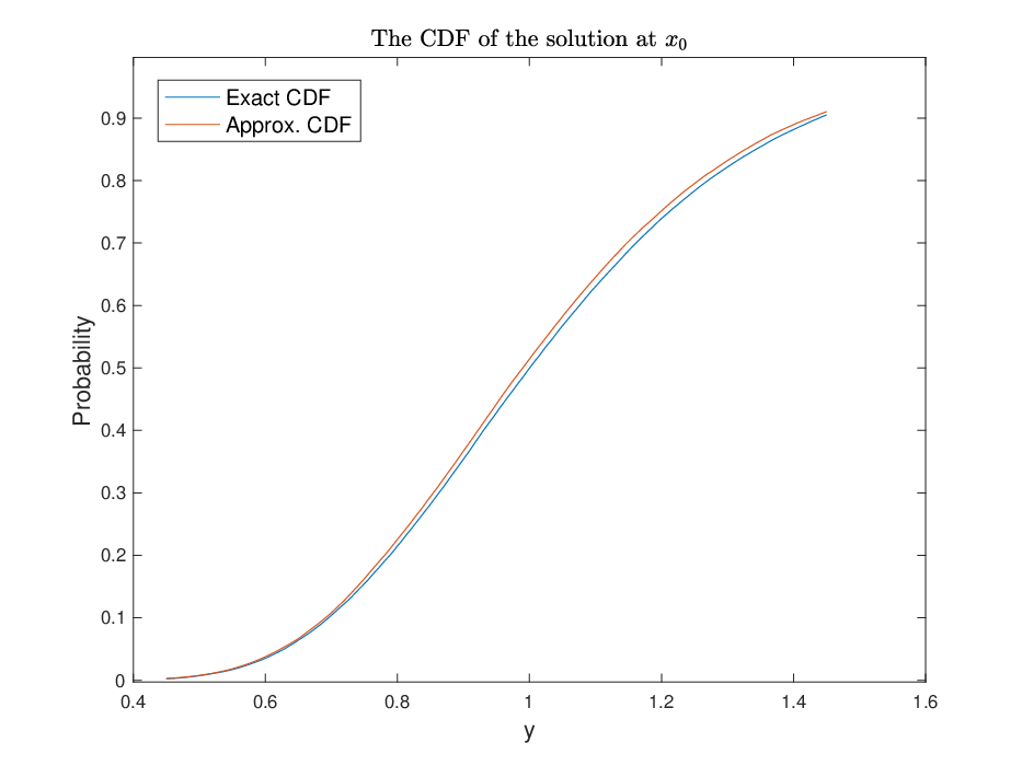
Finally, we assess the distribution of the approximated solution $u_{c}(x,{\bf Y})$ . To this end, we compare the CDF of the approximate solution $u_{c}$ and that of the exact solution $u$ at the point $x=0.5$ . The CDFs obtained by Monte Carlo simulation over $10^{5}$ samples are plotted in Figure 4.

5.3 Model semilinear problem with non-homogeneous random field

Finally, we study a semi-linear problem with non-homogeneous random field, i.e.,

\begin{split}-(\kappa(x,{\bf Y})u^{\prime}(x,{\bf Y}))^{\prime}+\sin(u(x,{\bf Y}))&=0,\qquad x\in D=[-l/2,l/2]\\ u(-l/2,{\bf Y})=u(l/2,{\bf Y})&=0,\end{split}

where $\kappa(x,{\bf Y})$ is the same log-normal random field as in the Section 5.1. Note that the exact solution is $u^{*}(x,{\bf Y})=0$ and hence the exact minimum value is $E(u^{*})=12$ . Over the finite dimensional space $V_{M}\otimes S_{N}$ , the functional is

J(c)=\mathbb{E}\left\{\int_{D}\frac{1}{2}\kappa(x,{\bf Y})(u_{c}^{\prime}(x,{\bf Y}))^{2}-\cos(u_{c}(x,{\bf Y}))\,dx\right\}.

The gradient estimator $g(x,{\bf Y})$ consists of two parts (see (11))

\begin{split}g_{i,j}^{1}(c,{\bf Y})&=\int_{D}\kappa(x,{\bf Y})u_{c}^{\prime}(x,{\bf Y})\phi_{i}^{\prime}(x)\Psi_{j}({\bf Y})\,dx,\\ g_{i,j}^{2}(c,{\bf Y})&=\int_{D}\sin(u_{c}(x,{\bf Y}))\phi_{i}(x)\Psi_{j}({\bf Y})\,dx\end{split}

for all $i=1,\cdots,M$ and $j=0,\cdots,N$ . Similarly, the Hessian estimator also has two parts

\begin{split}h_{(i_{1},j_{1}),(i_{2},j_{2})}^{1}(c,{\bf Y})&=\int_{D}\kappa(x,{\bf Y})\phi_{i_{1}}^{\prime}(x)\Psi_{j_{1}}({\bf Y})\phi_{i_{2}}^{\prime}(x)\Psi_{j_{2}}({\bf Y})\,dx\\ h_{(i_{1},j_{1}),(i_{2},j_{2})}^{2}(c,{\bf Y})&=\int_{D}\cos(u_{c}(x,{\bf Y}))\phi_{i_{1}}(x)\Psi_{j_{1}}({\bf Y})\phi_{i_{2}}(x)\Psi_{j_{2}}({\bf Y})\,dx\end{split}

for all $i_{1},i_{2}=1,\cdots,M$ and $j_{1},j_{2}=0,\cdots,N$ . Observe that the nonlinear part $h^{2}(c,{\bf Y})$ depends on the coefficient $c$ whereas the linear part $h^{1}(c,{\bf Y})$ does not. Hence, $h^{2}(c,{\bf Y})$ can be extremely noisy at the initial stage when SGD is still in its stochastic regime. The noisy estimation of $h^{2}(c,{\bf Y})$ in turn may have a detrimental rather than beneficial effect to guide the next search direction of SGD. In contrast, the linear part $h^{1}(c,{\bf Y})$ , although only contains partial second order information, is immune from the noisy updates of $c_{n}$ at the initial stage of SGD. This observation suggests that we can simply utilize the linear part of the Hessian estimator at the initial stage of SGD and incorporate the nonlinear part only after SGD gets stabilized. In Figure 5, we demonstrate the fast convergence behavior of SGD-PCE by incorporating the nonlinear part Hessian $h^{2}(c,{\bf Y})$ after $100$ iterations. In comparison, with the same learning rate, a naive use of the full Hessian information even does not lead to a converged result.

Finally, Figure 6 shows the effect of mini-batch sizes $N_{g}$ and $N_{h}$ on the convergence of SGD-PCE. The nonlinear part of Hessian is only incorporated after $100$ iterations. Recall that larger $\beta$ corresponds to larger variance of the random field $\kappa$ . When $\beta=0.3$ , mini-batch of size $128$ for gradient and $64$ for Hessian are not enough for SGD to converge in $500$ iterations. However, an increase of either $N_{g}$ or $N_{h}$ helps overcome the ill-conditioning issue of SGD. When $\beta=0.4$ , $128$ mini-batch samples for gradient estimation are not sufficient even when we increase $N_{h}$ to $128$ . However, the algorithm converges after we increase $N_{g}$ to $256$ , which suggests that SGD iteration is more tolerant to noise in the Hessian estimation than it is to the gradient estimation.

Summary and Conclusion

We have presented a variational framework for solving semilinear PDEs with random coefficients. The framework relies on the direct methods of variational calculus to recast the stochastic PDE as a stochastic minimization problem, which can then be solved by SGD over finite-dimensional subspaces. Our variational framework offers key advantages over traditional approaches based on weak formulations. First and foremost, from the theoretical standpoint, the direct methods of variational calculus automatically ensure weak convergence of the numerical solutions obtained under this framework. Second, our framework is able to take advantage of the countless SGD algorithms developed during the rapid ascend of machine learning in the last decade. Finally, the variational approach is well known to retain certain structures of the original problem and hence is particularly advantageous when applied to structure preserving problems. Based on this framework, we have proposed an SGD-PCE method utilizing the general PC expansion to approximate the stochastic space. By taking advantage of the special structure of the optimization problem derived from the PC expansion, we are able to design a version of SGD algorithm that finds the minimizer in an efficient way. We emphasize that, under our framework, other existing finite dimensional approximation techniques can be readily utilized in the same spirit. Despite the various advantages mentioned above, we are also aware of some weaknesses of our variational framework. For instance, the SGD-PCE can be computationally very costly, especially when the dimensionality of the approximation space $V_{M}\otimes S_{N}$ is high. Furthermore, a successful application of SGD in our framework requires careful tuning of multiple hyper-parameters, e.g. the learning rate, iteration number and mini-batch size. Often, such tuning is ad-hoc and hence can be very challenging for complex problems. In order to overcome these difficulties, it may be beneficial to apply more advanced variants of SGD such as the adaptive momentum (Adam) [21] algorithm capable of adaptively adjusting the learning rate and efficiently dealing with problems involving large set of parameters. This will be the focus of our future work.

Acknowledgments

The authors would like to thank Petr Plecháč and Gideon Simpson for fruitful discussions. The research of T.W. was sponsored by the CCDC Army Research Laboratory and was accomplished under Cooperative Agreement Number W911NF-16-2-0190. The views and conclusions contained in this document are those of the authors and should not be interpreted as representing the official policies, either expressed or implied, of the Army Research Laboratory or the U.S. Government. The U.S. Government is authorized to reproduce and distribute reprints for Government purposes notwithstanding any copyright notation herein.

References

[1] I. Babuška, F. Nobile, R. Tempone, A stochastic collocation method for elliptic partial differential equations with random input data, SIAM Journal on Numerical Analysis 45 (3) (2007) 1005–1034.
[2] F. Nobile, R. Tempone, C. G. Webster, A sparse grid stochastic collocation method for partial differential equations with random input data, SIAM Journal on Numerical Analysis 46 (5) (2008) 2309–2345.
[3] F. Nobile, R. Tempone, C. G. Webster, An anisotropic sparse grid stochastic collocation method for partial differential equations with random input data, SIAM Journal on Numerical Analysis 46 (5) (2008) 2411–2442.
[4] R. G. Ghanem, P. D. Spanos, Stochastic finite elements: a spectral approach, Courier Corporation, 2003.
[5] I. Babuska, R. Tempone, G. E. Zouraris, Galerkin finite element approximations of stochastic elliptic partial differential equations, SIAM Journal on Numerical Analysis 42 (2) (2004) 800–825.
[6] M. D. Gunzburger, C. G. Webster, G. Zhang, Stochastic finite element methods for partial differential equations with random input data, Acta Numerica 23 (2014) 521–650.
[7] D. Xiu, G. E. Karniadakis, The wiener–askey polynomial chaos for stochastic differential equations, SIAM journal on scientific computing 24 (2) (2002) 619–644.
[8] D. Xiu, G. E. Karniadakis, Modeling uncertainty in flow simulations via generalized polynomial chaos, Journal of computational physics 187 (1) (2003) 137–167.
[9] H. G. Matthies, A. Keese, Galerkin methods for linear and nonlinear elliptic stochastic partial differential equations, Computer methods in applied mechanics and engineering 194 (12-16) (2005) 1295–1331.
[10] F. Y. Kuo, D. Nuyens, Application of quasi-monte carlo methods to elliptic pdes with random diffusion coefficients: a survey of analysis and implementation, Foundations of Computational Mathematics 16 (6) (2016) 1631–1696.
[11] M. Struwe, Variational methods, Vol. 31999, Springer, 1990.
[12] J. N. Reddy, Energy principles and variational methods in applied mechanics, John Wiley & Sons, 2017.
[13] J. M. Ball, R. D. James, Fine phase mixtures as minimizers of energy, in: Analysis and Continuum Mechanics, Springer, 1989, pp. 647–686.
[14] S. Müller, Variational models for microstructure and phase transitions, in: Calculus of variations and geometric evolution problems, Springer, 1999, pp. 85–210.
[15] J. C. Simo, T. J. Hughes, Computational inelasticity, Vol. 7, Springer Science & Business Media, 2006.
[16] J. E. Marsden, M. West, Discrete mechanics and variational integrators, Acta Numerica 10 (2001) 357–514.
[17] B. Dacorogna, Direct methods in the calculus of variations, Vol. 78, Springer Science & Business Media, 2007.
[18] A. Nemirovski, A. Juditsky, G. Lan, A. Shapiro, Robust stochastic approximation approach to stochastic programming, SIAM Journal on optimization 19 (4) (2009) 1574–1609.
[19] L. Bottou, Large-scale machine learning with stochastic gradient descent, in: Proceedings of COMPSTAT’2010, Springer, 2010, pp. 177–186.
[20] L. Bottou, F. E. Curtis, J. Nocedal, Optimization methods for large-scale machine learning, Siam Review 60 (2) (2018) 223–311.
[21] D. P. Kingma, J. Ba, Adam: A method for stochastic optimization, arXiv preprint arXiv:1412.6980 (2014).
[22] H. Robbins, S. Monro, A stochastic approximation method, The annals of mathematical statistics (1951) 400–407.
[23] J. Mercer, Functions of positive and negative type, and their connection the theory of integral equations, Philosophical transactions of the royal society of London. Series A, containing papers of a mathematical or physical character 209 (441-458) (1909) 415–446.
[24] B. Oksendal, Stochastic differential equations: an introduction with applications, Springer Science & Business Media, 2013.
[25] O. Le Maıtre, O. Knio, H. Najm, R. Ghanem, Uncertainty propagation using wiener–haar expansions, Journal of computational Physics 197 (1) (2004) 28–57.
[26] O. Le Maıtre, H. N. Najm, R. Ghanem, O. Knio, Multi-resolution analysis of wiener-type uncertainty propagation schemes, Journal of Computational Physics 197 (2) (2004) 502–531.
[27] O. Le Maître, O. M. Knio, Spectral methods for uncertainty quantification: with applications to computational fluid dynamics, Springer Science & Business Media, 2010.
[28] A. Agarwal, P. L. Bartlett, P. Ravikumar, M. J. Wainwright, Information-theoretic lower bounds on the oracle complexity of stochastic convex optimization, IEEE Transactions on Information Theory 5 (58) (2012) 3235–3249.
[29] P. Zhao, T. Zhang, Accelerating minibatch stochastic gradient descent using stratified sampling, arXiv preprint arXiv:1405.3080 (2014).
[30] O. Dekel, R. Gilad-Bachrach, O. Shamir, L. Xiao, Optimal distributed online prediction using mini-batches, Journal of Machine Learning Research 13 (Jan) (2012) 165–202.
[31] J. Nocedal, S. Wright, Numerical optimization, Springer Science & Business Media, 2006.
[32] L. Bottou, Y. Le Cun, On-line learning for very large data sets, Applied stochastic models in business and industry 21 (2) (2005) 137–151.
[33] S.-I. Amari, Natural gradient works efficiently in learning, Neural computation 10 (2) (1998) 251–276.
[34] S.-I. Amari, H. Nagaoka, Methods of information geometry, Vol. 191, American Mathematical Soc., 2007.
[35] P. Glasserman, Monte Carlo methods in financial engineering, Vol. 53, Springer Science & Business Media, 2013.
[36] W. K. Liu, T. Belytschko, A. Mani, Random field finite elements, International journal for numerical methods in engineering 23 (10) (1986) 1831–1845.
[37] F. Yamazaki, M. Shinozuka, G. Dasgupta, Neumann expansion for stochastic finite element analysis, Journal of engineering mechanics 114 (8) (1988) 1335–1354.
[38] R. V. Field Jr, M. Grigoriu, J. Emery, On the efficacy of stochastic collocation, stochastic galerkin, and stochastic reduced order models for solving stochastic problems, Probabilistic Engineering Mechanics 41 (2015) 60–72.