Inclusive charged and neutral particle multiplicity distributions in and decays
Abstract
Using a sample of 106 million decays, and events are utilized to study inclusive anything, hadrons, and anything distributions, including distributions of the number of charged tracks, electromagnetic calorimeter showers, and s, and to compare them with distributions obtained from the BESIII Monte Carlo simulation. Information from each Monte Carlo simulated decay event is used to construct matrices connecting the detected distributions to the input predetection “produced” distributions. Assuming these matrices also apply to data, they are used to predict the analogous produced distributions of the decay events. Using these, the charged particle multiplicities are compared with results from MARK I. Further, comparison of the distributions of the number of photons in data with those in Monte Carlo simulation indicates that G-parity conservation should be taken into consideration in the simulation.
Keywords:
charmonium, , , inclusive distributions, Monte Carlo simulationpacs
07.05.Tp, 13.25.-k, 14.40.-nI Introduction
The multiplicity distributions of charged hadrons, which can be characterized by their means and dispersions, are an important observable in high energy collisions and an input to models of multihadron production. Charged particle means from below 2 GeV to LEP energies have been fit as a function of energy with a variety of models in Ref. opal, and a review of theoretical understanding can be found in Ref. carruthers.
The study of decays is important since they are expected to be an important source of glueballs, and future studies require both more data and better simulation of generic decays. Also since decays make up approximately 30% of decays, better understanding of decays improves that of decays.
The branching fractions of and were measured previously by BESIII using a sample of 106 million decays bam248. The accuracy of these measurements depends critically on the ability of the Monte Carlo (MC) simulation to model data well. Since a large fraction of hadronic decay modes are still unmeasured PDG, it is particularly important to verify the modeling of their inclusive decays, where we rely heavily on the LUNDCHARM model lundcharm to simulate these events.
In this paper, which is based on the analysis performed in Ref. bam248, we report on the “detected” distributions: the efficiency-corrected charged particle multiplicity distributions, as well as the efficiency-corrected distributions of the number of electromagnetic calorimeter showers and s for and decays. Our detected distributions are compared with MC simulation, and the results can be used to improve the LUNDCHARM model simulation, in particular for hadronic decays.
Information from each MC simulation decay event is used to construct matrices connecting the detected charged particle and photon multiplicity distributions to the input predetection distributions. Assuming the matrices also apply to data, they are used to predict the analogous “produced” distributions of the decay events. Produced charged particles and photons correspond to those coming directly from the or decays or the decays of their daughter particles. The means of the charged particle multiplicity distribution are compared with those of MARK I, which measured the mean charged particle multiplicity for hadrons as a function of center-of-mass energy from 2.6 to 7.8 GeV marki.
In Ref. bam248, an electromagnetic calorimeter (EMC) shower (EMCSH) was labeled a “photon”, but as described in Section IV.1, showers include hadronic interactions in the EMC crystals and electronic noise, so here we will explicitly refer to them as EMCSHs. The comparison of data and inclusive MC simulation showed good agreement for charged track distributions and most EMCSH energy () distributions, however, there was some difference in the distribution of the number of s bam248. Here, we explore the agreement for anything and hadrons via and anything via . Recently BESIII observed electromagnetic Dalitz decays lljp, so our hadron distributions also include . However, the branching fractions for these decays are very small, on the order of , which are negligible compared with those of hadrons. Below we will continue to refer to these distributions as hadrons. “Hadrons” is used very loosely and includes all processes except , such as other radiative decays and .
This analysis is based on the 106 million event sample gathered in 2009, the corresponding continuum sample with integrated luminosity of 44 pb-1 at GeV Npsip, and a 106 million event inclusive MC sample.
The paper is organized as follows: In Section II, the LUNDCHARM model is described. In Sections III - V, the distributions of the number of detected charged tracks, EMCSHs, and s, respectively, are determined and compared with MC simulation. Section VI presents the produced distributions. Section VII discusses systematic uncertainties, while Section VIII provides a summary. Additional EMCSH and tables are included in an appendix.
II LUNDCHARM model
The LUNDCHARM model is an event generator to produce events for charmonium decaying inclusively to anything lundcharm. This model, which was inspired by QCD theory, was developed at BESII and migrated to the BESIII experiment. In this model, or decaying into light hadrons is described as quark annihilation into one photon, three gluons or one photon plus two gluons, followed by the photon and gluons transforming into light quarks and further materializing into final light hadron states. To leading order accuracy, the quark annihilations are modeled by perturbative QCD pqcd, while the hadronization of light quark fragmentation is described with the Lund model pythia6.4 using a set of parameters to describe the baryon/meson ratio, strangeness and suppression, and the distribution of orbital angular momentum, etc.
| Charmonium | fraction of unmeasured decays |
|---|---|
| 0.1656 | |
| 0.8547 | |
| 0.5725 | |
| 0.7208 | |
| 0.5456 | |
| 0.7094 |
The LUNDCHARM model is used to generate the unmeasured charmonium decays, while the established decays are exclusively generated with their appropriate BesEvtGen models besevtgen using branching fractions from the Particle Data Group PDG. The fraction of unmeasured decays for each charmonium state is given in Table 1 PDG. Since the fractions are quite large for decays, the LUNDCHARM model is very important for the simulation of these decays. The parameters of the LUNDCHARM model are optimized using 20 million decays accumulated at the BESIII experiment tuning. Figure 1 shows the comparison between data and MC simulation of the multiplicity of detected charged tracks for and decays. More comparisons of data and MC simulation for decays can be found in Ref. tuning and for decays in Refs. tuning; bam248.


III Multiplicity distribution of charged tracks
III.1 Method
The basic approach is the same as in Ref. bam248. Charged tracks must be in the active region of the drift chamber and have their points of closest approach consistent with the run-by-run interaction point. Neutral tracks must be in the active regions of the barrel EMC or end-cap EMC, satisfy minimum and maximum energy requirements and a time requirement. The basic event selection requires at least one charged track (except for the study of the events with no charged tracks, where this requirement is dropped), at least one neutral track, and a minimum event energy. A background filter removes non- events, and events consistent with being a decay are removed bam248. Following this, the distribution is constructed for the remaining events, where the EMCSH must be in the barrel EMC, not originate from a charged track (, where is the angle between the shower and the nearest charged track), and not be a photon from a decay. Fitting the peaks in the distribution due to and , as shown in Fig. 2, allows the determination of the number of the inclusive decays and the final branching fractions. Please refer to Ref. bam248 for many important details.
To determine the distribution of the number of charged tracks, , ten distributions are constructed for ranging from 0 to 9. These distributions are then fitted to determine the numbers of anything and anything events, and these numbers determine the distributions for anything and anything.
In Ref. bam248, simultaneous fitting of inclusive and exclusive distributions was performed, but this is not done here, except for the case, because there are no exclusive distributions versus to be used in such a fit. Another change is that events with have additional requirements in order to reduce background in the distributions.
III.2 event selection and fit of distributions
Events with were selected in our previous analysis only to determine the systematic uncertainty associated with the requirement. The photon time requirement was removed since without charged tracks, the event time is not well determined. Although other selection requirements were tightened, the events still had much background bam248.
For the current analysis, events with GeV/ and GeV/ are removed, since these regions contain much background according to MC simulation. and are the sum of the momenta of all neutrals in the and directions, respectively, where and are orthogonal axes perpendicular to the axis of the detector. The distribution with the additional requirements is much cleaner and easily fitted, as shown in Fig. 2. A simultaneous fit with inclusive and exclusive events was used for the previous systematic uncertainty study since the signal to background ratio was so low, and the same fitting method is used here, as shown in Fig. 2. The for the fit to data is 1.3, where is the number of degrees of freedom.

III.3 selection and fitting
Figure 3 shows the distributions for all and for individual values of for data. distributions for different values of for MC simulation and continuum background are constructed similarly.
Signal shapes and background shapes used in the fit depend on the value of . In fitting the distributions for , because of the small sample sizes, the signal shapes and background shapes for are used. The fit result of data for is shown in Fig. 4, and the is 1.4. Fit results for other values of result in similar values.
The MC simulated sample is fitted as a function of in a similar fashion, but MC signal shapes are fitted without convolution. As described in Ref. bam248, the MC events are weighted by , where accounts for the difference between data and MC simulation on the number of s and accounts for the energy dependence of the radiative photon in the electric dipole transitions for and .


III.4 Results
The MC simulated sample is analyzed by counting the number of events versus before applying any selection criteria. The efficiency is then the number of events passing all selection criteria divided by the number of events without imposing any selection versus . Note that here is the “detected” number of charged tracks.
Using the number of detected data events, , and the MC determined efficiencies, , which are dependent on , we determine the distribution of the efficiency-corrected number of events in data for anything and anything. Results are listed in Table 2 for anything and Table 3 for anything.
For comparison, MC simulation numbers, , are also listed in the tables. corresponds to the distribution before imposing selection requirements. Since the branching fractions of MC simulation are not the same as the measured branching fractions of Ref. bam248, the MC numbers are scaled by , where and are the BESIII branching fractions bam248 and those used by the MC, respectively, and the in Tables 2 and 3 are the scaled MC numbers.
| (%) | (%) | (%) | ||||||||||
|---|---|---|---|---|---|---|---|---|---|---|---|---|
| 0 | 95664 | 30.7 | 311124 | 207332 | 73922 | 24.1 | 307213 | 218503 | 51006 | 21.1 | 241455 | 189395 |
| 1 | 206872 | 43.7 | 473186 | 450456 | 226613 | 43.6 | 519506 | 502988 | 165867 | 36.2 | 457732 | 446984 |
| 2 | 1003030 | 48.6 | 2065843 | 2041808 | 1210640 | 49.9 | 2426435 | 2414376 | 887474 | 41.9 | 2118574 | 2078609 |
| 3 | 663550 | 41.6 | 1594227 | 1782415 | 699804 | 41.5 | 1687651 | 1775014 | 589383 | 35.8 | 1646546 | 1790336 |
| 4 | 1602890 | 54.0 | 2969910 | 3100329 | 1662640 | 54.4 | 3058982 | 3031942 | 1459680 | 47.6 | 3064694 | 3073785 |
| 5 | 528842 | 47.3 | 1117174 | 1074490 | 566264 | 48.2 | 1173704 | 1137965 | 499056 | 42.0 | 1186940 | 1166188 |
| 6 | 502471 | 44.5 | 1128369 | 991170 | 533755 | 45.6 | 1171074 | 1046738 | 492290 | 40.0 | 1230654 | 1076283 |
| 7 | 70611 | 34.2 | 206487 | 124917 | 79957 | 35.4 | 225920 | 158769 | 76321 | 31.3 | 243714 | 163899 |
| 8 | 36744 | 25.9 | 141685 | 54033 | 38446 | 31.8 | 120915 | 73010 | 38390 | 27.5 | 139611 | 75074 |
| 9 | 2616 | 14.1 | 18570 | 3782 | 3087 | 24.0 | 12843 | 5478 | 3562 | 30.1 | 11845 | 5879 |
| (%) | (%) | |||||||
|---|---|---|---|---|---|---|---|---|
| 0 | 36983 | 28.9 | 128178 | 119881 | 19705 | 29.1 | 38250 | 65012 |
| 1 | 110869 | 47.2 | 234686 | 212706 | 60555 | 51.5 | 113737 | 119930 |
| 2 | 633989 | 54.3 | 1167955 | 1158351 | 320064 | 53.2 | 601156 | 633894 |
| 3 | 252917 | 47.7 | 530595 | 549543 | 136369 | 48.3 | 282565 | 297953 |
| 4 | 552012 | 59.7 | 925337 | 911111 | 294272 | 60.1 | 489386 | 516037 |
| 5 | 157700 | 53.1 | 297245 | 305425 | 83325 | 53.9 | 154712 | 163137 |
| 6 | 135463 | 49.0 | 276515 | 270788 | 73828 | 49.4 | 149512 | 157654 |
| 7 | 16602 | 36.9 | 44960 | 49716 | 8172 | 37.6 | 21736 | 22919 |
| 8 | 6724 | 28.4 | 23717 | 23877 | 2927 | 24.3 | 12033 | 12688 |
| 9 | 241 | 18.6 | 1296 | 1850 | 240 | 16.4 | 1463 | 1543 |
The efficiency corrected distributions for anything contain the anything events, as well as the hadrons events. A more interesting comparison between data and the simulated MC sample is with the distributions for hadrons directly. These are obtained by subtracting distributions for anything from those of anything. Since we do not have the distribution from data for anything, we use the MC distribution for this process. The branching fraction is small, 1.4 %, so the change for anything is small.
The fractions, , where the fraction is the number of efficiency corrected events with ( takes on values from 0 to 9) divided by the sum of all events, are determined and are listed in Table 4 for hadrons and Table 5 for anything. For comparison, MC simulation numbers, , are also listed in the tables. is calculated in an analogous way as was using the scaled MC simulation numbers. In Figs. 5 (a), (c), and (e) comparisons of the fractions between data and scaled MC simulated sample are shown, while Figs. 5 (b), (d), and (f) are the corresponding plots in logarithmic scale.
Figure 5 shows good agreement between the three anything decay distributions. Data are above MC simulation for and and below for for these distributions. The agreement between data and MC simulation is good for anything ( and ). Better agreement is expected for those distributions, since MC tuning was performed on the anything events.
| 0 | 2.09 | 1.46 | 1.54 | |||
|---|---|---|---|---|---|---|
| 1 | 4.56 | 4.29 | 4.05 | |||
| 2 | 20.62 | 18.58 | 17.89 | |||
| 3 | 18.17 | 18.12 | 18.48 | |||
| 4 | 31.63 | 31.37 | 31.67 | |||
| 5 | 10.97 | 12.31 | 12.42 | |||
| 6 | 10.12 | 11.48 | 11.38 | |||
| 7 | 1.27 | 1.61 | 1.75 | |||
| 8 | 0.55 | 0.73 | 0.77 | |||
| 9 | 0.04 | 0.05 | 0.05 |
| 0 | 3.33 | 3.27 | ||
|---|---|---|---|---|
| 1 | 5.90 | 6.02 | ||
| 2 | 32.15 | 31.84 | ||
| 3 | 15.25 | 14.97 | ||
| 4 | 25.29 | 25.92 | ||
| 5 | 8.48 | 8.19 | ||
| 6 | 7.52 | 7.92 | ||
| 7 | 1.38 | 1.15 | ||
| 8 | 0.66 | 0.64 | ||
| 9 | 0.05 | 0.08 |


IV Multiplicity distribution of the number of EMC showers
IV.1 MC study of EMC energy deposits
The situation for neutral showers is more complicated than for charged tracks. Energy deposits in the EMC from and events are caused by their radiative photons, photons from the decays of s from and hadronic decays and their daughter particles, bremsstrahlung from charged tracks, as well as interactions of hadrons in the EMC crystals and noise. The inclusive MC needs to model all these sources. We are interested in the number of photons, , from the hadronic decays of and . We can use the MC simulation to determine what fraction of the EMCSHs are due to radiative photons and the photons from the primary and secondary decays. We signify the number of EMCSHs by .
The MC “truth” information tags the radiative photons in the generator model and photons from the generator final particle decays in GEANT4 geant4, e.g. , as well as final-state radiation photons. MC truth does not tag the photons produced from the scattering and/or ionization of generator final state particles with the detector materials, simulated by GEANT4. The angles of tagged photons can be compared with the angles of EMCSHs to identify the fraction of showers that are caused by these photons. Figure 6 shows for a small subsample of events the angle , which is the minimum of the difference in angle between an EMCSH and all the MC tagged photons. There is a sharp peak at small corresponding to good shower matches between the MC predictions and the EMCSHs. We define showers with radians as a good shower match. The efficiency of matching photons in the correct angular range () and energy range (0.25 GeV 2 GeV) is 91.2%.

The fraction of good matches varies from 60% at the lowest energy to 89% at the highest. Figures 7 (a) and (b) show the number distributions of all and good showers, respectively. In the following, we will compare the distributions of data and MC simulation.


IV.2 distribution
The analysis for the distribution of is similar to that for . is the number of showers satisfying requirements on the energy, polar angle, and time, but no requirement on the angle between the shower and the closest charged track in the event. Here 15 energy distributions are constructed for ranging from 1 to , where is because at least one radiative photon must be detected. For more direct comparison of data with MC simulation, MC events are weighted only by .
As above, using the number of detected data events, , and the MC determined efficiencies, , versus , we determine the efficiency corrected distributions of data for anything and anything. Results are listed in Table 20 for anything and Table 21 for anything. The fractions, , are also determined and are listed in Table 6 for hadrons and Table 7 for anything. For comparison, MC simulation numbers, , are listed in Tables 20 and 21 in the appendix and fractions, , are listed in Tables 6 and 7.
| 1 | 6.37 | 4.33 | 4.75 | |||
|---|---|---|---|---|---|---|
| 2 | 9.51 | 8.11 | 8.39 | |||
| 3 | 14.20 | 13.40 | 13.49 | |||
| 4 | 17.28 | 16.76 | 16.82 | |||
| 5 | 17.69 | 17.86 | 17.70 | |||
| 6 | 13.63 | 14.74 | 14.42 | |||
| 7 | 9.48 | 10.71 | 10.44 | |||
| 8 | 5.79 | 6.71 | 6.63 | |||
| 9 | 3.20 | 3.80 | 3.76 | |||
| 10 | 1.58 | 1.95 | 1.95 | |||
| 11 | 0.74 | 0.94 | 0.94 | |||
| 12 | 0.32 | 0.42 | 0.42 | |||
| 13 | 0.14 | 0.17 | 0.18 | |||
| 14 | 0.05 | 0.07 | 0.08 | |||
| 0.02 | 0.03 | 0.03 |
| 1 | 3.78 | 4.12 | ||
|---|---|---|---|---|
| 2 | 12.56 | 12.21 | ||
| 3 | 11.58 | 11.77 | ||
| 4 | 15.16 | 15.03 | ||
| 5 | 15.19 | 15.06 | ||
| 6 | 13.75 | 13.75 | ||
| 7 | 10.98 | 10.96 | ||
| 8 | 7.65 | 7.62 | ||
| 9 | 4.49 | 4.53 | ||
| 10 | 2.47 | 2.50 | ||
| 11 | 1.28 | 1.31 | ||
| 12 | 0.63 | 0.65 | ||
| 13 | 0.30 | 0.31 | ||
| 14 | 0.13 | 0.13 | ||
| 0.05 | 0.05 |


In Figs. 8 (a), (c), and (e) the comparisons of the fractions between data and the scaled MC simulated sample are shown, and Figs. 8 (b), (d), and (f) are the corresponding plots in logarithmic scale. For hadrons, the distributions in Fig. 8 are similar for the three decays, and data are above MC simulation for and and below for and 6. For anything ( and ), there is only minor disagreement between data and MC simulation for the distributions.
V Multiplicity distribution of the number of s
An even more complicated case is the distribution of the number of s, . Here, as for the case, the distribution is considered in more detail. The invariant mass, , distribution of the candidates is shown in Fig. 9, where there are a large number of miscombinations in the plot. A somewhat better estimate of is made with the restrictive requirement 0.145 GeV, which was the requirement used when vetoing EMCSHs that might be part of a combination from the distribution used in the fitting for the number of and events bam248. However, even with this requirement there are still many miscombinations.
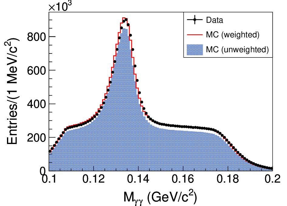
To determine the fraction, , of the candidates that are valid s, we fit the distributions for 0.145 GeV for each for both data and the MC simulated sample to a signal shape and first order Chebychev polynomial background. The basic signal shape was determined using the MC truth information to identify correct combinations in simulated data. For data, the basic signal shape is convolved with a bifurcated Gaussian function to account for the difference in resolution between data and the MC simulated sample. is the fraction of signal events in the region 0.145 GeV. The values of versus are listed in Table 8.
Note that may not fully determine the number of valid s. For instance, may include the cases of three valid s, two valid s and one miscombination, one valid and two miscombinations, and three miscombinations.
| (%) | (%) | |
|---|---|---|
| all | ||
| 0 | 100 (assumed) | 100 (assumed) |
| 1 | ||
| 2 | ||
| 3 | ||
| 4 | ||
| 5 | ||
| 6 | ||
| 7 | ||
| 8 | ||
| 9 |
The analysis for the detected distributions is similar to those for and . Here 10 distributions of data are constructed for ranging from 0 to . For more direct comparison of data with MC simulation, MC events are weighted only by .
Using the number of detected data events, , the MC determined efficiencies, , and versus , we determine the efficiency corrected distributions of data for anything and anything, where , which gives a better representation of the distribution. Results are listed in the appendix in Table 22 for anything and Table 23 for anything. The fractions, , are also determined and are listed in Table 9 for hadrons and Table 10 for anything. For comparison, scaled MC simulation numbers, , multiplied by are listed in Tables 22 and 23 and MC fractions, , are listed in Tables 9 and 10.
| 0 | 45.53 | 44.79 | 44.27 | |||
|---|---|---|---|---|---|---|
| 1 | 31.27 | 29.57 | 29.37 | |||
| 2 | 14.08 | 14.09 | 14.32 | |||
| 3 | 5.29 | 6.18 | 6.36 | |||
| 4 | 2.16 | 2.80 | 2.91 | |||
| 5 | 0.92 | 1.30 | 1.38 | |||
| 6 | 0.40 | 0.62 | 0.68 | |||
| 7 | 0.18 | 0.31 | 0.34 | |||
| 8 | 0.08 | 0.16 | 0.17 | |||
| 0.07 | 0.18 | 0.20 |
| 0 | 54.72 | 53.29 | ||
|---|---|---|---|---|
| 1 | 25.16 | 25.23 | ||
| 2 | 10.79 | 11.25 | ||
| 3 | 4.80 | 5.14 | ||
| 4 | 2.24 | 2.46 | ||
| 5 | 1.09 | 1.23 | ||
| 6 | 0.56 | 0.63 | ||
| 7 | 0.29 | 0.34 | ||
| 8 | 0.16 | 0.19 | ||
| 0.20 | 0.25 |


In Figs. 10 (a), (c), and (e) comparisons of the fractions between data and scaled MC simulated samples are shown, and Figs. 10 (b), (d), and (f) provide logarithmic versions. For hadrons, the distribution, data are above MC simulation for . For anything ( and ), data are above MC simulation for , but the uncertainties are bigger for these decays.
VI Produced distributions
So far, we have only dealt with the distributions of the efficiency-corrected number of detected charged tracks, EMCSHs, or pions. These depend on the geometry and performance of the BESIII detector. Of more interest are the actual physics distributions in the decays of the and .
To determine these distributions from data, we construct detection matrices using the hadrons and anything events in the inclusive MC events. The matrix () times the produced vector () determines the detected vector (), where () is the number of events with charged tracks, photons, or s, etc.
| (1) |
The elements of are determined using the MC “truth” information by tallying the detected versus the produced track information for each event. The detection matrix is then assumed to apply to data, as well as to MC simulation. Detected histograms are constructed corresponding to each element in the vector using the matrix equation (1). These are used to give a set of probability density functions (PDFs) with which to perform a fit of the detected distributions of data to determine the values for .
VI.1 distributions
The results of the fits to the detected charged track distributions of data to determine the produced charged track distributions are shown in Fig. 11 for hadrons. Here refers to the number of produced tracks. Shown in Figs. 11 (a) - (c) are the MC fractions and the results from the fits to the detected distributions of data. Charge conservation requires that be even. Shown in Figs. 11 (d) - (f) are the detected data fractions and the fractions determined from the fit results, as well as the PDFs used in the fits. The distributions in Figs. 11 (a) - (c) are similar, and the fit results are below the MC fractions for and somewhat above for and .


Results for anything are shown in Fig. 12. Shown in Figs. 12 (a) - (b) are the MC fractions and the results from the fits to the detected distributions of data. Shown in Figs. 12 (c) - (d) are the detected data fractions and the fit results, as well as the PDFs used in the fits. The distributions in Figs. 12 (a) - (b) are similar, and the fitted fractions are in reasonable agreement with the MC fractions.


In Figs. 11 (d) - (f) and Figs. 12 (c) - (d), 9 bins of detected data are fitted with 6 parameters ( through ) and with fixed to the MC values. Fractions of hadrons and anything are listed in Tables 11 and 12, respectively. The values for the five cases are 65, 52, 85, 18, and 28. Alternative fits with free give the same results as shown in Tables 11 and 12. Comparing the fits and the PDFs in Figs. 11 and 12 suggests that the MC PDFs do not describe data well, which contributes to the large . However, corrections to the PDFs to improve the fits to the detected charged track distributions, as described in Section VII, result in small changes to the values compared with the systematic uncertainties shown in Table 19 and are neglected.
| 0 | 1.41 | 0.86 | 0.94 | |||
| 2 | 21.55 | 19.04 | 17.92 | |||
| 4 | 49.61 | 48.67 | 49.53 | |||
| 6 | 25.11 | 28.30 | 28.31 | |||
| 8 | 2.27 | 3.07 | 3.23 | |||
| 10 | 0.05 | 0.07 | 0.08 | |||
| 12 | 0 | 0 | 0 |
| 0 | 2.07 | 1.99 | ||
| 2 | 36.68 | 35.08 | ||
| 4 | 39.92 | 39.68 | ||
| 6 | 18.35 | 19.37 | ||
| 8 | 2.91 | 3.67 | ||
| 10 | 0.06 | 0.21 | ||
| 12 | 0 | 0 |
Mean charged multiplicity and dispersion

| (GeV) | ||||
|---|---|---|---|---|
| hadrons | ||||
| hadrons | ||||
| hadrons | ||||
| hadrons | ||||
| hadrons |
We determine values of the mean multiplicity , dispersion , and . Such measurements have been performed for hadrons at LEP opal, and also at lower energies with the MARK I experiment marki. The results of these measurements from our data are listed in Table 13. Although we measure anything via anything, we can calculate the hadron distribution using the branching fractions of and PDG and assuming that these events populate only. The calculated values are also listed in Table 13.
Our values for can be compared with those of MARK I for hadrons marki. The MARK I values from 2.8 to 4.0 GeV are plotted in Fig. 13 along with our values for both and to hadrons. While our results include statistical and systematic uncertainties, those of MARK I do not include systematic uncertainties, which range from 25% at 2.6 GeV to 15% at 6 GeV and above. Still, the agreement between the results is very good.
VI.2 distributions
distributions are studied in an analogous way. Here the distributions correspond to the MC-tagged photons, described in Section IV, and the detected distributions are the EMC shower distributions, which include both good and bad shower matches. The results of the fits for the distributions are shown in Fig. 14 for hadrons. Shown in Figs. 14 (a) - (c) are the MC fractions and the results from the fits to the detected distributions of data. The radiative photons from are not counted, so the lowest bin is . Even bins are much larger than odd ones since most photons are from decays. Photons from final-state radiation (FSR) and radiative photons from intermediate-state decays are counted and contribute to odd bins. While fit results for bins 2, 6, and 10 are smaller than MC, those for 0, 4, 8, and 12, which correspond to an even number of s, are much larger than MC. The detected data fractions as a function of and the fractions determined from the fit results are shown in Figs. 14 (d) - (f).


Results for anything are shown in Fig. 15. The MC fractions and the results from the fits to the detected distributions of data are shown in Figs. 15 (a) - (b). Since radiative photons from and are not counted, the lowest bin is also . Here, for bins with 2, 6, and 10, which correspond to a preference for an odd number of s, fit results are slightly larger than MC, but uncertainties are large. The detected data fractions versus and the fit results are shown in Figs. 15 (c) - (d). The -parity for s is positive, suggesting that decays to pions should favor an even number of s, while -parity for the is negative, implying that decays to pions favor an odd number of s. These preferences in the distributions of the number of photons are observed above for data, but MC simulation does not reflect this.
In Figs. 14 (d) - (f) and Figs. 15 (c) - (d), 14 bins of detected data are being fit with 7 parameters (, , , , , , and ) with in-between bins fixed to MC values. The number of degrees of freedom is = 7. Fractions of hadrons are listed in Table 14 and anything are listed in Table 15. The values for the five cases are 17, 7.8, 4.3, 5.7, and 2.9.
| 0 | 17.66 | 14.29 | 14.40 | |||
| 1 | 1.61 | 1.57 | 1.44 | |||
| 2 | 23.48 | 24.31 | 24.59 | |||
| 3 | 2.72 | 2.89 | 2.87 | |||
| 4 | 28.45 | 27.51 | 27.90 | |||
| 5 | 3.15 | 3.42 | 3.37 | |||
| 6 | 13.64 | 15.61 | 14.95 | |||
| 7 | 1.90 | 2.09 | 2.06 | |||
| 8 | 5.00 | 5.39 | 5.54 | |||
| 9 | 0.55 | 0.68 | 0.69 | |||
| 10 | 1.25 | 1.56 | 1.50 | |||
| 11 | 0.17 | 0.18 | 0.19 | |||
| 12 | 0.32 | 0.34 | 0.36 | |||
| 13 | 0.11 | 0.14 | 0.15 |
| 0 | 21.60 | 20.57 | ||
| 1 | 5.15 | 5.92 | ||
| 2 | 28.82 | 27.61 | ||
| 3 | 5.03 | 6.18 | ||
| 4 | 14.76 | 14.28 | ||
| 5 | 4.11 | 4.61 | ||
| 6 | 11.69 | 11.39 | ||
| 7 | 2.17 | 2.64 | ||
| 8 | 4.22 | 4.11 | ||
| 9 | 0.57 | 0.74 | ||
| 10 | 0.84 | 0.84 | ||
| 11 | 0.21 | 0.23 | ||
| 12 | 0.65 | 0.64 | ||
| 13 | 0.18 | 0.22 |
VI.3 distributions
distributions are studied in a similar fashion. Here, the situation is complicated because events for a given contain miscombinations as well as real s. We assume that the MC simulation correctly describes the miscombinations in data and do not multiply by . Unlike the cases above, the alternate bins are not suppressed, so adjacent PDFs are similar in shape, which results in larger fit uncertainties for the values of .
The low sensitivity that the fit has to has other consequences. For most of the variations used in Section VII to determine systematic uncertainties, the fits of the detected distributions of data fail, with only three successful fits out of a total of nine. See Section VII for details. In conclusion, we are not able to determine the systematic uncertainties for the distributions corresponding to the detected distributions and therefore the event fractions themselves.
VI.4 Input-Output Check
The procedures above have been repeated using MC detected distributions as input. The output produced distributions determined by the analyses should then agree closely with the MC truth distributions. We divide the MC data in half and use the first half to construct the detection matrices and use them in fitting the detected distributions of the second half. We compare the fitting results with the MC truth fractions of the second half. For this check, the uncertainties on the detected distributions are taken as the statistical uncertainties on the number of detected events combined in quadrature with the statistical uncertainties on the number of MC events. The output fitted fractions and input MC fractions versus are given in Table 16, where the agreement is very good. The values for the fits are 1.2, 0.9, 0.8, 0.5, and 0.7.
The output fitted fractions and input MC fractions versus are given in Table 17. The agreement for these cases is not as good as for the cases. The values for are 1.2, 0.5, 0.2, 1.5, and 2.2. In all cases, the differences between input and output are small compared to the systematic uncertainties detailed in Table 19 and are neglected.
| 0 | 1.413 | 0.854 | 0.930 | 2.068 | 1.985 | |||||
|---|---|---|---|---|---|---|---|---|---|---|
| 2 | 21.56 | 19.07 | 17.94 | 36.71 | 35.14 | |||||
| 4 | 49.61 | 48.66 | 49.49 | 39.94 | 39.68 | |||||
| 6 | 25.10 | 28.28 | 28.33 | 18.31 | 19.32 | |||||
| 8 | 2.271 | 3.062 | 3.229 | 2.911 | 3.655 | |||||
| 10 | 0.048 | 0.069 | 0.081 | 0.063 | 0.205 |
| 0 | 17.67 | 14.28 | 14.41 | 21.62 | 20.55 | |||||
|---|---|---|---|---|---|---|---|---|---|---|
| 1 | 1.60 | 1.57 | 1.44 | 5.15 | 5.92 | |||||
| 2 | 23.49 | 24.34 | 24.61 | 28.82 | 27.61 | |||||
| 3 | 2.72 | 2.89 | 2.87 | 5.04 | 6.18 | |||||
| 4 | 28.42 | 27.49 | 27.87 | 14.75 | 14.28 | |||||
| 5 | 3.15 | 3.43 | 3.39 | 4.11 | 4.61 | |||||
| 6 | 13.64 | 15.62 | 14.96 | 11.69 | 11.40 | |||||
| 7 | 1.91 | 2.08 | 2.06 | 2.16 | 2.65 | |||||
| 8 | 5.00 | 5.40 | 5.52 | 4.21 | 4.13 | |||||
| 9 | 0.55 | 0.68 | 0.69 | 0.57 | 0.74 | |||||
| 10 | 1.25 | 1.56 | 1.49 | 0.84 | 0.83 | |||||
| 11 | 0.17 | 0.18 | 0.19 | 0.21 | 0.23 | |||||
| 12 | 0.32 | 0.34 | 0.36 | 0.66 | 0.63 | |||||
| 13 | 0.11 | 0.14 | 0.15 | 0.18 | 0.22 |
VII Systematic Uncertainties
Extensive studies of systematic uncertainties were carried out in Ref. bam248. For the branching fraction, they are under 4 % with the largest contribution coming from fitting the distribution. Many of the uncertainties do not apply here. For the distribution of the number of charged tracks, the uncertainty from does not apply, since we include events with no charged tracks. The requirement essentially includes all events, as does , which has a small systematic uncertainty. The uncertainty from does not apply since we calculate event fractions. Those for MC signal shape, multipole correction, and affect the selection of the radiative photon candidate and the overall number of events, but should not affect the various distributions.
Systematic uncertainties are determined here for detected event fractions in Sections III - V and for produced event fractions in Sections VI.1 - VI.2 using samples selected with alternate selection criteria and with modified fitting procedures. Systematic uncertainties are the differences from the standard procedure added in quadrature.
For all distributions, the fitting uncertainties are determined by changing the background polynomial, changing the range, and fixing small signals. Background polynomials are changed from second order to first, and the fit ranges are changed from 0.08-0.5 GeV to 0.08-0.35 GeV and 0.2-0.54 GeV.
For the detected charged track event fraction systematic uncertainties in Section III and the fraction uncertainties in Section VI.1, (a) the fitting uncertainties are considered, and in addition, uncertainties from (b) the background veto, (c) the veto, (d) the requirement, and (e) the continuum energy difference are determined. The uncertainties from (b) - (d) are determined by removing those requirements and comparing with the analyses making them. The uncertainty from (e) is determined by scaling the EMCSH energies of the continuum events by the ratio of the center-of-mass energies of data and the continuum data.
For the detected photon event fraction systematic uncertainties in Section IV, the event fraction systematic uncertainties in Section VI.2, and the detected pion event fraction uncertainties in Section V, the fitting errors are considered. In addition, uncertainties from the background veto, the veto, the requirement, and continuum energy difference are determined.
An important question is what are the systematic uncertainties associated with the determination of the produced distributions by fitting the detected distributions in Section VI. We study this in two ways. In the first, we modify the PDFs used in determining the values. In Section VI.1 the fits have large , and the PDFs in Figs. 11 (d) - (f) and Figs. 12 (c) - (d) do not appear to describe the detected distributions of data well. Data are above the fit in the highest bin and below in the preceding bin for the and PDFs in Figs. 11 (d) - (f) and Figs. 12 (c) - (d). The PDFs determined from the inclusive MC seem to be too broad.
The PDFs have been modified to see the effect on the s and further to determine the differences in the results. We assume that part of the PDFs may be described approximately by a binomial distribution. For instance, we assume that the PDF for for through can be described by a binomial distribution in terms of an efficiency , which includes the geometric, tracking, and vertexing efficiencies, and the fraction of in through is given according to a binomial distribution by . The PDFs of the MC being too wide is due to the efficiences being too small. We estimate the corrected efficiency approximately by comparing the data fractions and the fitted fractions for the bins in Figs. 11 (d) - (f) and Figs. 12 (c) - (d), , where is the data fraction bin content of and is the fitted fraction bin content. For Fig. 11 (d), and ; the difference is only 0.64%. We then use the ratio of the binomial distributions in terms of the two efficiencies in each bin to correct the MC PDFs and use the corrected PDFs to fit the detected distributions. The part of the PDF for is left unchanged. We do analogous calculations for and .
The corrected PDFs fit the detected distributions much better now than they did in Figs. 11 and 12, and the s become 15.5, 12.3, 17.7, 5.4, and 9.0, which are much reduced compared to those in Section VI.1 (65, 52, 85, 18, and 28). The differences with the uncorrected fractions are small compared with the systematic uncertainties shown in Table 19 and are neglected.
In the second, more quantitative study, we modify the selection criteria for both charged tracks and EMCSHs by requiring that they satisfy , corresponding to the barrel shower counter. The detected distributions are greatly altered by such a requirement. This is easy to understand: the probability of removing a charged track goes way up when there are a large number of charged tracks. The detected distributions are pushed to lower values, while the produced truth distributions of MC are not affected. For example, the means of the detected distributions are 3.82, 3.58, and 3.68 (3.20, 3.14, and 3.25) for the standard () selection for , , and hadrons, while the means of the produced distributions are 4.27, 4.44, and 4.46 (4.28, 4.44, and 4.48), respectively, for the standard () selection. The differences with the standard selection for both and values are taken as the systematic uncertainties associated with the determination of the produced distributions by fitting the detected distributions.
The detected event fraction uncertainties and the event fraction uncertainties are listed in Tables 18 and 19, respectively. The uncertainties are the individual uncertainties for all cases added in quadrature.
| 0 | 9.63 | 20.1 | 7.57 | 16.4 | 28.1 | 0 | 3.01 | 3.50 | 7.64 | 6.21 | 14.6 | ||||||
|---|---|---|---|---|---|---|---|---|---|---|---|---|---|---|---|---|---|
| 1 | 7.70 | 5.97 | 4.59 | 21.9 | 16.3 | 1 | 4.82 | 5.04 | 3.34 | 12.5 | 22.4 | 1 | 4.91 | 3.33 | 7.40 | 4.41 | 12.0 |
| 2 | 1.98 | 1.10 | 1.48 | 3.94 | 8.23 | 2 | 6.49 | 3.37 | 4.76 | 6.43 | 10.5 | 2 | 6.64 | 3.24 | 7.68 | 14.7 | 8.09 |
| 3 | 2.69 | 1.47 | 1.19 | 6.44 | 5.77 | 3 | 2.21 | 2.53 | 3.62 | 5.28 | 9.28 | 3 | 7.84 | 2.70 | 4.90 | 9.75 | 14.4 |
| 4 | 1.80 | 1.07 | 1.92 | 3.96 | 6.79 | 4 | 2.36 | 1.54 | 3.06 | 8.75 | 9.13 | 4 | 17.9 | 7.49 | 9.11 | 16.9 | 23.0 |
| 5 | 5.74 | 2.61 | 2.70 | 10.2 | 10.3 | 5 | 3.21 | 2.05 | 3.71 | 7.86 | 17.4 | 5 | 10.2 | 6.61 | 13.2 | 13.8 | 20.1 |
| 6 | 2.91 | 2.21 | 1.50 | 6.66 | 7.90 | 6 | 4.61 | 1.71 | 3.02 | 6.40 | 7.02 | 6 | 12.8 | 6.37 | 15.0 | 44.9 | 14.4 |
| 7 | 30.4 | 14.0 | 11.0 | 16.9 | 27.8 | 7 | 5.79 | 3.30 | 3.40 | 6.59 | 14.0 | 7 | 145 | 100 | 103 | 146 | 210 |
| 8 | 5.60 | 8.01 | 16.3 | 40.4 | 22.2 | 8 | 9.04 | 4.60 | 4.48 | 12.1 | 24.7 | 8 | 151 | 143 | 188 | 179 | 414 |
| 9 | 126 | 43.3 | 75.3 | 457 | 374 | 9 | 24.4 | 8.28 | 10.1 | 11.7 | 21.1 | 9 | 60.6 | 102 | 344 | 144 | 270 |
| 10 | 41.9 | 13.0 | 12.0 | 27.5 | 24.3 | ||||||||||||
| 11 | 28.7 | 18.5 | 10.4 | 29.7 | 59.6 | ||||||||||||
| 12 | 39.3 | 26.3 | 50.5 | 52.0 | 73.5 | ||||||||||||
| 13 | 57.5 | 35.6 | 43.5 | 57.0 | 47.4 | ||||||||||||
| 14 | 96.5 | 33.1 | 55.4 | 114 | 188 |
| 0 | 0.49 | 1.50 | 0.76 | 0.81 | 4.14 | 0 | 1.33 | 3.09 | 0.69 | 2.05 | 3.50 |
|---|---|---|---|---|---|---|---|---|---|---|---|
| 2 | 0.78 | 6.80 | 3.57 | 1.57 | 3.91 | 1 | 0.02 | 0.01 | 0.20 | 0.03 | 0.08 |
| 4 | 1.11 | 2.99 | 1.37 | 2.81 | 6.34 | 2 | 2.59 | 7.27 | 5.30 | 5.57 | 10.1 |
| 6 | 2.17 | 3.92 | 2.27 | 1.64 | 3.09 | 3 | 0.03 | 0.01 | 0.39 | 0.03 | 0.08 |
| 8 | 4.66 | 4.19 | 1.94 | 2.35 | 2.57 | 4 | 3.98 | 12.56 | 8.50 | 11.8 | 20.7 |
| 10 | 3.11 | 2.65 | 1.43 | 2.64 | 1.62 | 5 | 0.03 | 0.01 | 0.46 | 0.03 | 0.06 |
| 12 | 0 | 0 | 0 | 0 | 0 | 6 | 8.61 | 9.08 | 6.30 | 9.95 | 17.0 |
| 7 | 0.02 | 0.01 | 0.28 | 0.01 | 0.04 | ||||||
| 8 | 9.02 | 9.63 | 4.26 | 4.11 | 5.74 | ||||||
| 9 | 0.01 | 0.00 | 0.09 | 0.00 | 0.01 | ||||||
| 10 | 2.98 | 7.38 | 0.00 | 1.76 | 4.07 | ||||||
| 11 | 0.00 | 0.00 | 0.03 | 0.00 | 0.00 | ||||||
| 12 | 2.09 | 2.62 | 1.51 | 0.92 | 0.08 | ||||||
| 13 | 0.00 | 0.00 | 0.02 | 0.00 | 0.00 |
VIII Summary
The study of decays is important since they are expected to be a source for glueballs, and their simulation is a necessary part of their understanding. Since a large fraction of their hadronic decay modes are unmeasured, the close modeling of their inclusive decays is very important.
Using 106 million decays, we study anything, hadrons, and anything distributions. Distributions of event fractions for data are compared with MC simulation versus the number of detected charged tracks, EMCSHs and s in Figs. 5, 8 and 10, respectively. For all comparisons, the agreement is reasonable. However, there are differences.
To start with anything, for the distributions, data are above MC simulation for and and below for and 6. For the distributions, data are above MC simulation for and and below for , and for the distributions, data are above MC simulation for .
For anything ( and ), the agreement between data and MC simulation is good for the distributions. There is some disagreement for the distributions, and for the distributions data are above MC simulation for , but the uncertainties are bigger. Better agreement is expected for anything distributions, since MC tuning was performed on the anything events.
For hadron charged track distributions, fit results shown in Fig. 11 for are below the MC fractions for and above for and . results for anything charged track distributions are shown in Fig. 12. The distributions are similar, and the fit fractions are in reasonable agreement with the MC fractions. The means of the above distributions in Figs. 11 and 12 are determined and plotted along with results from MARK I for hadrons in the same energy range in Fig. 13. The charmonium decays to hadrons and hadrons results are consistent.
The results for the distributions are shown in Fig. 14 (a) - (c) for hadrons. The content of even bins are much larger than those of odd ones since most photons are from the decay of s. While fit results for bins 2, 6, and 10 are smaller than MC, those for 0, 4, 8, and 12, which correspond to an even number of s, are much larger than MC. Results for anything for photons are shown in Fig. 15. Here, bins with 2, 6, and 10, which correspond to a preference for an odd number of s, appear to have fit results slightly larger than MC.
The -parity for s is positive, suggesting that decays should favor an even number of s, while -parity for the is negative, implying that decays favor an odd number of s. These preferences in the distributions of the number of produced photons are observed for data, but MC simulation does not adequately reflect this.
While the agreement between data and MC simulation is reasonable at present, it should be improved for future studies of decays and measurements of the branching fractions with even larger data sets. This can be accomplished with further MC tuning or by weighting the present or future MC simulation to give better agreement with data.
Acknowledgements.
The BESIII collaboration thanks the staff of BEPCII and the IHEP computing center for their strong support. This work is supported in part by National Key Basic Research Program of China under Contract No. 2015CB856700; National Natural Science Foundation of China (NSFC) under Contracts Nos. 11625523, 11635010, 11735014, 11822506, 11835012; the Chinese Academy of Sciences (CAS) Large-Scale Scientific Facility Program; Joint Large-Scale Scientific Facility Funds of the NSFC and CAS under Contracts Nos. U1532257, U1532258, U1732263, U1832207; CAS Key Research Program of Frontier Sciences under Contracts Nos. QYZDJ-SSW-SLH003, QYZDJ-SSW-SLH040; 100 Talents Program of CAS; INPAC and Shanghai Key Laboratory for Particle Physics and Cosmology; ERC under Contract No. 758462; German Research Foundation DFG under Contracts Nos. Collaborative Research Center CRC 1044, FOR 2359, GRK 214; Istituto Nazionale di Fisica Nucleare, Italy; Koninklijke Nederlandse Akademie van Wetenschappen (KNAW) under Contract No. 530-4CDP03; Ministry of Development of Turkey under Contract No. DPT2006K-120470; National Science and Technology fund; STFC (United Kingdom); The Knut and Alice Wallenberg Foundation (Sweden) under Contract No. 2016.0157; The Royal Society, UK under Contracts Nos. DH140054, DH160214; The Swedish Research Council; U. S. Department of Energy under Contracts Nos. DE-FG02-05ER41374, DE-SC-0010118, DE-SC-0012069; University of Groningen (RuG) and the Helmholtzzentrum fuer Schwerionenforschung GmbH (GSI), DarmstadtReferences
- (1)
- (2) P. D. Acton et al. (OPAL Collaboration), Z. Phys. C 53, 539 (1992).
- (3) P. Carruthers and C. C. Shih, International Journal of Modern Physics A, Vol. 2, 1447 (1987).
- (4) M. Ablikim et al. (BESIII Collaboration), Phys. Rev. D 96, 032001 (2017).
- (5) M. Tanabashi et al. (Particle Data Group), Phys. Rev. D 98, 030001 (2018).
- (6) J. C. Chen, G. S.Huang, X. R. Qi, D. H. Zhang, Y. S. Zhu et al., Phys. Rev. D 62, 034003 (2000).
- (7) J. L. Siegrist et al. (MARK I Collaboration), Phys. Rev. D 26, 969 (1982).
- (8) M. Ablikim et al. (BESIII Collaboration), Phys. Rev. D 99, 051101 (2019).
- (9) M. Ablikim et al. (BESIII Collaboration), Chin. Phys. C 37, 063001 (2013)
- (10) L. Kopke and N. Wermes, Phys. Rept. 174, 67 (1989).
- (11) T. Sjostrand, S. Mrenna, and P. Z. Skands, JHEP 0605, 026 (2006).
- (12) R. G. Ping, Chin. Phys. C 32, 599 (2008).
- (13) R. L. Yang, R. G. Ping, and H. Chen, Chin. Phys. Lett. 31, 061301 (2014).
- (14) S. Agostinelli et al. (GEANT4 Collaboration), Nucl. Instrum. Meth. A 506, 250 (2003).
*
Appendix A Additional Material
| (%) | (%) | (%) | ||||||||||
|---|---|---|---|---|---|---|---|---|---|---|---|---|
| 1 | 330758 | 49.4 | 669238 | 615384 | 229324 | 47.4 | 483430 | 427139 | 237868 | 44.7 | 532591 | 461904 |
| 2 | 439022 | 47.6 | 921785 | 926793 | 531929 | 51.8 | 1027261 | 996329 | 416190 | 46.2 | 901025 | 913571 |
| 3 | 638938 | 49.7 | 1286718 | 1375251 | 700129 | 54.0 | 1295902 | 1316389 | 596027 | 47.7 | 1250544 | 1314188 |
| 4 | 803512 | 49.9 | 1609754 | 1674111 | 883514 | 53.4 | 1655182 | 1671070 | 761699 | 46.5 | 1638571 | 1645770 |
| 5 | 846497 | 51.6 | 1640005 | 1712936 | 888728 | 51.8 | 1717062 | 1745654 | 776282 | 45.1 | 1719400 | 1716841 |
| 6 | 589146 | 49.1 | 1198819 | 1322729 | 683444 | 48.4 | 1411174 | 1483861 | 556411 | 41.5 | 1340519 | 1428027 |
| 7 | 412950 | 46.1 | 895086 | 921471 | 489771 | 44.8 | 1093266 | 1113650 | 383015 | 37.7 | 1016905 | 1053385 |
| 8 | 272287 | 42.2 | 645279 | 564767 | 308651 | 40.3 | 765307 | 725934 | 241913 | 33.4 | 724569 | 681520 |
| 9 | 148286 | 37.2 | 398285 | 311757 | 168098 | 34.9 | 482143 | 416583 | 127628 | 28.4 | 449811 | 390813 |
| 10 | 68326 | 32.8 | 208052 | 154672 | 802275 | 29.4 | 273469 | 219793 | 56201 | 23.7 | 237515 | 205847 |
| 11 | 30494 | 24.4 | 125022 | 72763 | 33641 | 26.2 | 128294 | 108885 | 26640 | 19.4 | 137025 | 100920 |
| 12 | 13037 | 23.7 | 55089 | 31841 | 14393 | 19.4 | 74292 | 50682 | 11927 | 15.7 | 76107 | 46826 |
| 13 | 6089 | 23.0 | 26495 | 13265 | 5171 | 17.0 | 30430 | 22417 | 4627 | 10.0 | 46364 | 20569 |
| 14 | 3549 | 25.8 | 13768 | 5385 | 1945 | 14.2 | 13659 | 9332 | 1810 | 6.6 | 27262 | 8646 |
| 1810 | 31.1 | 5824 | 2103 | 769 | 13.8 | 5564 | 3664 | 98 | 11.4 | 857 | 3263 |
| (%) | (%) | |||||||
|---|---|---|---|---|---|---|---|---|
| 1 | 37240 | 24.0 | 155156 | 135859 | 20743 | 25.7 | 44857 | 80865 |
| 2 | 235504 | 48.8 | 483059 | 451104 | 104954 | 46.2 | 192872 | 239863 |
| 3 | 228811 | 54.3 | 421096 | 415890 | 117186 | 54.4 | 215350 | 231364 |
| 4 | 298314 | 58.9 | 506781 | 544528 | 157503 | 58.9 | 267321 | 295275 |
| 5 | 294228 | 57.7 | 510057 | 545477 | 159820 | 58.2 | 274596 | 295923 |
| 6 | 271070 | 56.8 | 477675 | 493600 | 147040 | 57.1 | 257544 | 270282 |
| 7 | 217292 | 54.5 | 399037 | 394206 | 116281 | 55.3 | 210384 | 215396 |
| 8 | 141923 | 51.2 | 276988 | 274819 | 75507 | 51.8 | 145684 | 149717 |
| 9 | 76562 | 45.1 | 169632 | 161328 | 41794 | 45.8 | 91345 | 89043 |
| 10 | 33602 | 38.6 | 87068 | 88704 | 21989 | 39.5 | 55648 | 49176 |
| 11 | 15673 | 29.2 | 53626 | 45834 | 10894 | 39.7 | 27438 | 25702 |
| 12 | 5588 | 26.9 | 20780 | 22788 | 4294 | 27.4 | 15701 | 12718 |
| 13 | 1657 | 13.1 | 12771 | 10753 | 1328 | 27.3 | 4858 | 6165 |
| 14 | 611 | 9.9 | 6145 | 4545 | 324 | 12.6 | 2566 | 2558 |
| 374 | 22.1 | 1693 | 1809 | 0 | 8.9 | 0 | 976 |
| (%) | (%) | (%) | ||||||||||
|---|---|---|---|---|---|---|---|---|---|---|---|---|
| 0 | 2120810 | 54.7 | 3877450 | 3895611 | 2361620 | 59.9 | 3944259 | 4008941 | 1960130 | 54.6 | 3592178 | 3669625 |
| 1 | 1394550 | 50.9 | 2199410 | 2307965 | 1502400 | 52.6 | 2295310 | 2322469 | 1288210 | 46.4 | 2228712 | 2271990 |
| 2 | 674368 | 42.2 | 1075983 | 1023269 | 679189 | 39.3 | 1164391 | 1071370 | 584461 | 32.7 | 1202462 | 1091068 |
| 3 | 261673 | 32.0 | 458967 | 406560 | 274281 | 28.7 | 536108 | 471751 | 219636 | 22.4 | 551204 | 486484 |
| 4 | 111118 | 24.6 | 226317 | 174196 | 115964 | 20.9 | 277841 | 215496 | 88399 | 15.6 | 284253 | 224716 |
| 5 | 47410 | 17.7 | 122876 | 78627 | 47504 | 15.2 | 143682 | 101846 | 36508 | 10.8 | 154817 | 107356 |
| 6 | 20810 | 12.8 | 67830 | 36456 | 19718 | 11.0 | 74533 | 49819 | 14077 | 6.62 | 88404 | 53125 |
| 7 | 10644 | 9.17 | 46153 | 17555 | 7856 | 7.45 | 41914 | 25008 | 5895 | 5.22 | 44884 | 26762 |
| 8 | 5628 | 9.00 | 23078 | 8819 | 3690 | 4.92 | 27678 | 13039 | 2736 | 3.64 | 27714 | 14105 |
| 8981 | 9.33 | 31171 | 9703 | 3144 | 3.68 | 27662 | 15608 | 2943 | 1.69 | 56302 | 16785 |
| (%) | (%) | |||||||
|---|---|---|---|---|---|---|---|---|
| 0 | 891038 | 56.7 | 1571227 | 1618965 | 433812 | 55.8 | 750852 | 854740 |
| 1 | 529136 | 57.4 | 740963 | 744487 | 280425 | 57.8 | 445982 | 404714 |
| 2 | 251421 | 49.3 | 343268 | 319198 | 139981 | 50.5 | 219284 | 180373 |
| 3 | 113103 | 41.4 | 153318 | 141990 | 67755 | 43.0 | 88476 | 82390 |
| 4 | 48556 | 32.7 | 74432 | 66240 | 31190 | 34.5 | 45360 | 39462 |
| 5 | 19321 | 22.0 | 40334 | 32237 | 13517 | 28.2 | 21982 | 19692 |
| 6 | 9178 | 15.1 | 25304 | 16500 | 5976 | 20.4 | 12195 | 10144 |
| 7 | 4218 | 11.1 | 15110 | 8508 | 3076 | 14.5 | 8431 | 5405 |
| 8 | 1927 | 10.3 | 6925 | 4640 | 1165 | 9.77 | 4401 | 2998 |
| 955 | 2.58 | 11978 | 6053 | 223 | 2.70 | 2678 | 4024 |