Robust Variational Autoencoding with Wasserstein Penalty for Novelty Detection
Chieh-Hsin Lai∗ Dongmian Zou∗ Gilad Lerman
School of Mathematics, University of Minnesota Division of Natural and Applied Sciences, Duke Kunshan University School of Mathematics, University of Minnesota
Abstract
We propose a new method for novelty detection that can tolerate high corruption of the training points, whereas previous works assumed either no or very low corruption. Our method trains a robust variational autoencoder (VAE), which aims to generate a model for the uncorrupted training points. To gain robustness to high corruption, we incorporate the following four changes to the common VAE: 1. Extracting crucial features of the latent code by a carefully designed dimension reduction component for distributions; 2. Modeling the latent distribution as a mixture of Gaussian low-rank inliers and full-rank outliers, where the testing only uses the inlier model; 3. Applying the Wasserstein-1 metric for regularization, instead of the Kullback-Leibler (KL) divergence; and 4. Using a robust error for reconstruction. We establish both robustness to outliers and suitability to low-rank modeling of the Wasserstein metric as opposed to the KL divergence. We illustrate state-of-the-art results on standard benchmarks.
1 INTRODUCTION
Machine learning solutions often assume that training datasets are flawless and can serve as ground truth. However, this assumption usually does not hold in practice. Indeed, most datasets, even commonly used ones such as CIFAR-10 or ImageNet, suffer from corruption and mislabeling (Northcutt et al. 2021). While in many applications the percentage of mislabels may be sufficiently small, there are important scenarios where this is not the case. One such scenario appears when studying problems with no earlier experience and expertise. For instance, in the beginning of the COVID-19 pandemic it was hard to diagnose COVID-19 patients and distinguish them from other patients with pneumonia (Chowdhury et al. 2020; Xiao et al. 2020). Another scenario occurs when it is very hard to make precise measurements, for example, when working with the highly corrupted images in cryogenic electron microscopy (cryo-EM) (Miolane et al. 2020; Huang & Tagare 2015).
One problem, where it is crucial to carefully address mislabeled training data points, is novelty detection. It asks to detect testing data points that deviate from the underlying structure of a given training dataset (Chandola et al. 2009; Pimentel et al. 2014; Chalapathy & Chawla 2019; Perera et al. 2021). Novelty detection is equivalent to the well-known one-class classification problem (Moya & Hush 1996). This problem asks to identify members of a class in a test dataset, and consequently distinguish them from “novel” data points, given training points from this class. The points of the main class are commonly referred to as inliers and the novel ones as outliers. Novelty detection is also commonly referred to as semi-supervised anomaly detection. In this terminology, the notion of being “semi-supervised” is different from usual, and means that a training set is provided for the inliers only. On the other hand, the supervised case has labeled training data for both the inliers and outliers, and the unsupervised case has no training and is also known as “outlier detection”.
Traditional one-class classification methods often assume that the training set is purely sampled from a single class or has few outliers and perform poorly when there is a nontrivial portion of outliers. In this paper, we study a robust version of novelty detection that allows a nontrivial fraction of corrupted samples, namely outliers, within the training set. We solve this problem by using a special variational autoencoder (VAE) (Kingma & Welling 2014). Our VAE is able to model the underlying distribution of the uncorrupted data, despite nontrivial corruption. We refer to it as “Mixture Autoencoding with Wasserstein penalty”, or “MAW”.
1.1 Previous Work
Solutions to novelty detection either estimate the density of the inlier distribution (Bengio & Monperrus 2005; Ilonen et al. 2006) or determine a geometric property of the inliers, such as their boundary set (Breunig et al. 2000; Schölkopf et al. 2000; Xiao et al. 2016; Wang & Lan 2020; Jiang et al. 2019). When the inlier distribution is nicely approximated by a low-dimensional linear subspace, Shyu et al. 2003 propose to distinguish between inliers and outliers via Principal Component Analysis (PCA). In order to consider more general cases of nonlinear low-dimensional structures, one may use autoencoders (or restricted Boltzmann machines), which nonlinearly generalize PCA (Goodfellow et al. 2016, Ch. 2) and whose reconstruction error naturally provides a score for membership in the inlier class. Instances of this strategy with various architectures include (Zhai et al. 2016; Zong et al. 2018; Sabokrou et al. 2018; Perera et al. 2019; Pidhorskyi et al. 2018). In all of these works, but (Zong et al. 2018), the training set is assumed to solely represent the inlier class. If there are also outliers (with a simple shape) among the inliers (with a complex shape), encoding the inlier distribution becomes difficult. Nevertheless, some previous works already explored the possibility of a corrupted training set (Xiao et al. 2016; Wang & Lan 2020; Zong et al. 2018). In particular, Xiao et al. 2016; Zong et al. 2018 test artificial instances with at most corruption of the training set and Wang & Lan 2020 consider ratios of , but with very small numbers of training points. In this work we consider corruption ratios up to , with a method that tries to estimate the distribution of the training set, and not just a geometric property.
VAEs (Kingma & Welling 2014) have been commonly used for generating distributions with reconstruction scores and are thus natural for novelty detection without corruption. The first VAE-based method for novelty detection was suggested by An & Cho 2015. It was recently extended by Daniel et al. 2021 who modified the training objective. A variety of VAE models were also proposed for special anomaly detection problems, which are different from novelty detection (Xu et al. 2018; Zhang et al. 2019; Pol et al. 2019). Current VAE-based methods for novelty detection do not perform well when the training data is corrupted. Indeed, the learned distribution of any such method also represents corruption, that is, the outlier component. To the best of our knowledge, no effective solutions were proposed for collapsing the outlier mode so that the trained VAE would only represent the inlier distribution.
A variant of VAE is the adversarial autoencoder (AAE) of (Makhzani et al. 2016). The penalty term of AAE takes the form of a generative adversarial network (GAN) (Goodfellow et al. 2016), where the AAE’s encoder serves as the GAN’s generator. We can thus view it as a hybrid GAN-VAE model. Another such model is the Wasserstein autoencoder (WAE) (Tolstikhin et al. 2018), which generalizes AAE by allowing a general objective function. Our proposed model is also a hybrid GAN-VAE. Other hybrid VAE-GAN models include (Mescheder et al. 2017; Xian et al. 2019; Ye & Bors 2021). The GAN of (Mescheder et al. 2017) is used for both the samples and the latent code, the GAN of (Xian et al. 2019; Ye & Bors 2021) is used only for the samples, whereas the GAN of our work and (Makhzani et al. 2016; Tolstikhin et al. 2018) is used only for the latent code. We demonstrate the resulting robustness to outliers due to our particular use of a GAN.
There are two relevant lines of work on robustness to outliers in linear modeling that can be used in nonlinear settings via autoencoders or VAEs. Robust PCA aims to deal with sparse elementwise corruption of a data matrix (Candès et al. 2011; De La Torre & Black 2003; Wright et al. 2009; Vaswani & Narayanamurthy 2018). Robust subspace recovery (RSR) aims to address general corruption of selected data points and thus better fits the framework of outliers (Watson 2001; De La Torre & Black 2003; Ding et al. 2006; Zhang et al. 2009; McCoy & Tropp 2011; Xu et al. 2012; Lerman & Zhang 2014; Zhang & Lerman 2014; Lerman et al. 2015; Lerman & Maunu 2017; Maunu et al. 2019; Lerman & Maunu 2018; Maunu & Lerman 2019). Autoencoders that use robust PCA for anomaly detection tasks were proposed in (Chalapathy et al. 2017; Zhou & Paffenroth 2017). It is shown in (Dai et al. 2018) that a VAE can be interpreted as a nonlinear robust PCA problem. Nevertheless, explicit regularization is often required to improve robustness to sparse corruption in VAEs (Akrami et al. 2019; Eduardo et al. 2020). An RSR layer was successfully applied to outlier detection in (Lai et al. 2020). One can also apply this work to novelty detection.
We remark that the setting of our work is different from that of out-of-distribution (OOD) detection and open-set recognition. Indeed, in these recent settings the inliers are from multiple classes that need to be identified. On the other hand, this work does not ask to classify the inliers.
1.2 This Work
We propose a robust novelty detection procedure, MAW, that aims to model the distribution of the training data in the presence of a nontrivial fraction of outliers. We highlight its following four features:
- 1.
MAW models the latent distribution by a Gaussian mixture of low-rank inliers and full-rank outliers, and applies the inlier distribution for testing. Previous applications of mixture models for novelty detection were designed for multiple modes of inliers and used more complicated tools such as additional network construction (Zong et al. 2018) or clustering (Aytekin et al. 2018; Lee et al. 2018).
- 2.
MAW applies a novel dimension reduction component, which extracts lower-dimensional features of the latent distribution. The reduced dimension allows using full covariances; whereas previous VAE-based methods for novelty detection used diagonal covariances in their models (An & Cho 2015; Daniel et al. 2021).
- 3.
MAW uses the Wasserstein-1 () metric for the latent code penalty. We prove that the Wasserstein metric gives rise to outlier-robust estimation and is suitable to the low-rank modeling of inliers by MAW. We also show that these properties do not hold for the commonly-used KL divergence. To the best of our knowledge, this is the first theoretical analysis that clarifies the advantage of the Wasserstein distance over the KL divergence in a VAE in terms of robustness to outliers and low-rank inlier modeling.
- 4.
MAW achieves state-of-the-art results on popular anomaly detection datasets.
Additional two features are as follows. First, for reconstruction, MAW replaces the common least squares formulation with a least absolute deviations formulation. This can be justified by the use of a robust estimator (Lopuhaa & Rousseeuw 1991) with a heavier-tail likelihood. Second, MAW is attractive for practitioners. It is simple to implement in any standard deep learning library, and is easily adaptable to other choices of network architecture, energy functions and similarity scores.
2 DESCRIPTION OF MAW
We motivate and overview the underlying model and assumptions of MAW in §2.1. We describe the implementation details of its components in §2.2 and sketch the algorithm procedures in the supplementary materials. Fig. 1 illustrates the general idea of MAW and can assist in reading this section.

2.1 The Model and Assumptions of MAW
MAW aims to robustly estimate a mixture inlier-outlier distribution for the training data and then use its inlier component to detect outliers in the testing data. For this purpose, it designs a novel variational autoencoder with an underlying mixture model and a robust loss function in the latent space. We find the variational framework natural for novelty detection. Indeed, it learns a distribution that describes the inlier training examples and generalizes to the inlier test data. Moreover, the variational formulation allows a direct modeling of a Gaussian mixture model (GMM) in the latent space, unlike a standard autoencoder.
Let be a random variable in with an unknown training data distribution, which contains both inlier and outlier modes. We assume training points in , sampled from this distribution. We assume a latent random variable of low and even dimension (our default choice is ), and a standardized Gaussian prior, , so that . In the remaining text, we shall denote it as
The posterior distribution is unknown. However, we assume an approximation to it, which we denote by
| (1) |
where depend on and are generated by the encoder network and the dimension reduction component (explained below) the default choice for the mixture parameter is (the low sensitivity of our method to the choice of is demonstrated in the supplementary materials). The first mode in (1) represents the inliers and the second one represents the outliers. We model as a single Gaussian since we only want to include the inlier information, while having the simplest possible design. In §4.3, we will numerically compare with the modeling of as a GMM. In the supplementary materials we intuitively clarify the mechanism that helps in such modeling.
The dimension reduction component involves a mapping from a higher-dimensional space onto the latent space. It is analogous to the RSR layer (Lai et al. 2020) that projects encoded points onto the latent space, but requires a more careful design since we consider a distribution rather than sample points. Due to this reduction, we assume that the mapped covariance matrices of are full, unlike common single-mode VAE models that assume a diagonal covariance (Kingma & Welling 2014; An & Cho 2015). We assume that the inliers lie on a low-dimensional structure and we thus enforce the lower rank for , but allow to have full rank . Nevertheless, we later describe a necessary regularization of both matrices. We remark that the low rank assumption results in the main distinction between the inliers and outliers in (1) (as noted in the supplementary materials the choice of is not crucial).
The unknown posterior distribution is approximated within the variational family indexed by , , and . Unlike a standard VAE, which maximizes the evidence lower bound (ELBO), MAW maximizes the following loss function, which uses the distance (defined in the supplementary materials), instead of the KL divergence, for regularizing the log-likelihood of the data distribution:
| (2) |
We use the Wasserstein distance since it is more robust to outliers than the KL divergence and is thus more suitable for detecting anomalies (see related guarantees in §3).
Following the VAE framework, we use a Monte-Carlo approximation to estimate with i.i.d. samples, , from as follows:
| (3) |
To enhance robustness, we let the negative log likelihood function be proportional to the norm of the difference of the random variable and a mapping of the sample from to by the decoder, , that is,
| (4) |
We deviate from the common choice of the squared norm, which corresponds to an underlying Gaussian likelihood and assume instead a likelihood with a heavier tail.
MAW trains its networks by minimizing . For , it samples from , where all samples are independent. Using the aggregation formula , the approximation of by the empirical distribution of the training data, and (2)-(4), MAW applies the following approximation of :
| (5) |
During testing, MAW identifies outliers according to low similarity scores computed between test points and points generated from the learned inlier component of .
2.2 Details of Implementing MAW
MAW has a VAE-type structure with additional WGAN-type structure for minimizing the loss in (5). We provide here details of implementing these structures. Some specific choices of the networks are described in §4 since they may depend on the type of datasets.
The VAE-type structure of MAW contains three ingredients: encoder, dimension reduction component and decoder. The encoder forms a neural network (NN), , that maps the training sample in to in , where our default choice is . The dimension reduction component then computes the following statistical quantities of the GMM : means and in and covariance matrices and in . First, a linear layer, represented by , maps (via ) the features , to the following respective vectors in :
The mapping of the covariance matrices is constructed as follows. Form for . For , compute . For , we first need to reduce the rank of . For this purpose, we form
| (6) |
the spectral decomposition of , and then truncate its bottom eigenvalues. That is, let have the same entries as the largest entries of and zero entries otherwise. Then, compute
| (7) |
and
To ensure numerically-significant positive definiteness of both and , we add to them an identity matrix. Despite this, the low-rank structure of is still evident. Note that the dimension reduction component only trains . The decoder, , maps independent samples, , generated for each by the distribution
into the reconstructed data space.
The loss function associated with the VAE structure is the first term in (5). We can write it as
| (8) |
The dependence of this loss on and is implicit, but follows from the fact that the parameters of the sampling distribution of each were obtained by and .
The WGAN-type structure seeks to minimize the second term in (5) using the dual formulation
| (9) | ||||
The generator of this WGAN-type structure is composed of the encoder and the dimension reduction component, which we represent by . It generates the samples described above. The discriminator, , of the WGAN-type structure plays the role of the Lipschitz function in (9). It compares the latter samples with the i.i.d. samples from the prior distribution. In order to make Lipschitz, its weights are clipped to during training. In the MinMax game of this WGAN-type structure, the discriminator minimizes and the generator ( and ) maximizes
| (10) |
We note that maximization of (10) by the generator is equivalent to minimization of the loss function
| (11) |
During training, MAW alternatively minimizes the losses (8), (10) and (11) instead of their weighted sum. Therefore, any multiplicative constant in front of either term of (5) will not affect the optimization. In particular, it was okay to omit the multiplicative constant of (4) when deriving (5).
For each testing point , we sample from the inlier mode of the learned latent Gaussian mixture and decode them as . Using a similarity measure (our default is the cosine similarity), we compute
If is larger than a chosen threshold, then is classified as normal, and otherwise, novel. Additional details of MAW are in the supplementary materials.
We remark that in our setting we find it natural to implement an auxiliary WGAN on top of the VAE component in order to estimate the distance. We did not find it useful to directly estimate the distance by either the sliced Wasserstein distance (Kolouri et al. 2018; Kolouri et al. 2019) or the Sinkhorn algorithm (Cuturi 2013). Indeed, it is not clear how to use these methods in order to minimize the estimated distance with respect to the parameters within the neural network. In particular, the partial derivatives for learning the GMM using the sliced Wasserstein distance already have very complicated forms, and it is very difficult to include them in our framework, where neural networks are involved.
3 THEORETICAL GUARANTEES
We theoretically establish the superiority of using the Wasserstein distance over the KL divergence, where we leave out some details (in particular proofs) to the supplementary materials. We formulate a mathematical setting that aims to isolate the minimization of the WGAN-type structure introduced in §2.2, while ignoring unnecessary complex components of MAW. We assume a mixture parameter , a separation parameter and denote by the regularizing function, which can be either the KL divergence or the Wasserstein distance, and by and the sets of positive semidefinite and positive definite matrices, respectively. Our mathematical setting, which we motivate in the supplementary materials, assumes and and requires to minimize
| (12) | ||||
This minimization aims to approximate the “prior” distribution with a Gaussian mixture distribution. For MAW, and , but our generalization helps clarify things. The constraint distinguishes between the inlier and outlier modes and it is a realistic assumption as long as is sufficiently small.
3.1 Guarantees for (12) with Identical Covariances
Our cleanest result is when , and coincide. It is formulated next and demonstrates robustness to the outlier component by the (or , ) minimization and not by the KL minimization (its proof is in the supplementary materials).
Proposition 3.1
That is, under the above setting with , the estimated mean of the inlier distribution, , coincides with the mean of the prior distribution, independently of the outlier distribution. However, when , the estimated mean of the inlier distribution is sensitive to outliers.
3.2 Guarantees for (12) with Low-rank
We study the minimization problem (12) when has a low rank and . We fully analyze the cases where and ; however, the case where is difficult to analyze and compute. We first formulate results for both cases ( and ), and then clarify them. When , we assume that the prior distribution has zero mean vector and covariance . We further denote by the vector . Similarly, we denote for any , , , . For vectors and , we denote the concatenated vector in by .
Proposition 3.2
If , , , , , , where one can note that and , then the minimizer of (12) with and the constraints that is of rank and is of rank , satisfies , and . Moreover, and .
Proposition 3.3
If , , , , , , , and , rank, then
Thus, the solution of (12) with and the additional constraints and is ill-posed.
Note that Proposition 3.2 implies that as , . Hence for the inlier component as and . Therefore, in the limit, the inlier distribution has the same mean as the prior distribution. Furthermore, its covariance is obtained by an appropriate projection of the covariance onto a -dimensional subspace, independently of . We similarly note that as , , so that the outliers disperse. The supplementary materials include the proof of Proposition 3.2 and a discussion that clarifies why the formulation and proof of Proposition 3.2 are not sufficient for inferring the effect of the minimization on MAW.
Proposition 3.3 implies that the KL divergence is unsuitable for low-rank covariance modeling as it leads to an infinite value in the optimization problem.
4 EXPERIMENTS
We describe the competing methods and experimental choices in §4.1. We report on the comparison with the competing methods in §4.2. We demonstrate the importance of the novel features of MAW in §4.3.
4.1 Competing Methods and Experimental Choices
We compared MAW with the following methods (descriptions and code links are in the supplementary materials): Deep Autoencoding Gaussian Mixture Model (DAGMM) (Zong et al. 2018), Deep Structured Energy-Based Models (DSEBMs) (Zhai et al. 2016), Isolation Forest (IF) (Liu et al. 2008), Local Outlier Factor (LOF) (Breunig et al. 2000), One-class Novelty Detection Using GANs (OCGAN) (Perera et al. 2019), One-Class SVM (OCSVM) (Heller et al. 2003) and RSR Autoencoder (RSRAE) (Lai et al. 2020).
We remark that IF, LOF and RSRAE were originally proposed for outlier detection and we thus apply their trained model for detecting novelties in the test data.
For MAW and the above four reconstruction-based methods, that is, DAGMM, DSEBMs, OCGAN and RSRAE, we use the following structure of encoders and decoders, which vary with the type of data (images or non-images). For non-images, which are mapped to feature vectors of dimension , the encoder is a fully connected network with output channels . The decoder is a fully connected network with output channels , followed by a normalization layer at the end. For image datasets, the encoder has three convolutional layers with output channels , kernel sizes and strides . Its output is flattened to lie in and then mapped into a dimensional vector using a dense layer (with output channels ). The decoder of image datasets first applies a dense layer from to and then three deconvolutional layers with output channels , kernel sizes and strides . For all experiments, the MAW discriminator is a fully connected network with size .
For MAW we set the following parameters, where additional details are in the supplementary materials. Intrinsic dimension: ; mixture parameter: , sampling number: , and size of (used for dimension reduction): . We further test the sensitivity of MAW to changes of the hyperparameters and in the supplementary materials. The code is available at https://github.com/JCL823/MAW.
4.2 Comparison of MAW with State-of-the-art Methods

We use six datasets for novelty detection: COVID-19 Radiography database (Chowdhury et al. 2020), CIFAR-10 (Krizhevsky 2009), Caltech101 (Fei-Fei et al. 2004), Fashion MNIST (Xiao et al. 2017), KDDCUP-99 (Dua & Graff 2017) and Reuters-21578 (Lewis 1997). We distinguish between image datasets (COVID-19, CIFAR-10, Catlech101 and Fashion MNIST) and non-image datasets (KDDCUP-99 and Reuters-21578). We describe each dataset, common preprocessing procedures and choices of their largest clusters in the supplementary materials. Each dataset contains several clusters (3 for COVID-19, 10 for CIFAR-10, 11 largest ones for Caltech101, 10 for Fashion MNIST, 2 for KDDCUP-99 and 5 largest ones for Reuters-21578, respectively). We arbitrarily fix a class and uniformly sample training inliers and testing inliers from that class. We let , , , , , and , , , , , for COVID-19, CIFAR-10, Caltech101, Fashion MNIST, KDDCUP-99 and Reuters-21578, respectively. We fix in , and uniformly sample outliers for training from the rest of the clusters, while maintaining a fraction of outliers per inliers. We also fix in and uniformly sample outliers from the rest of the clusters for testing, while maintaining a fraction of per inliers.
Using all possible thresholds for the finite datasets, we compute the AUC (area under curve) and AP (average precision) scores, while considering the outliers as “positive”. For each fixed , , , , we average these results over the values of , the different choices of an inlier cluster (among all possible clusters), and three runs with different random initializations for each of these choices. We also compute the corresponding standard deviations. We report these results in Fig. 2 and further specify numerical values in the supplementary materials. We observe state-of-the-art performance of MAW in all of these datasets. There are very special instances, where other methods perform better, for example, in Reuters-21578, DSEBMs performs slightly better than MAW and OCSVM has comparable performance. However, overall MAW is the most competitive method considering all instances. In the supplementary materials we compare the runtime of MAW with benchmark methods and further study the accuracy of MAW in a different scenario, where the outliers of the training and test sets have different characteristics. We show that in this scenario MAW performs even better than the regular scenario.
4.3 Testing the Effect of the Novel Features of MAW
We experimentally validate the effect of the following features of MAW: the least absolute deviation for reconstruction, the metric for the regularization of the latent distribution, the GMM assumption, full covariance matrices resulting from the dimension reduction component, the lower rank constraint for the inlier mode and the use of a single mode prior distribution. To this end, we consider the following alternative models.
MAW-MSE: It replaces the least absolute deviation loss with the common mean squared error (MSE).
MAW-KL divergence: It replaces the Wasserstein distance in (9) with the KL-divergence.
MAW-same rank: It uses the same rank for both and , instead of forcing to have lower rank .
MAW-single Gaussian: It replaces the GMM for the latent distribution with a single Gaussian with a full covariance matrix.
MAW-diagonal cov.: It replaces the full covariance matrices resulting from the dimension reduction component by diagonal covariances. Its encoder directly produces 2-dimensional means and diagonal covariances (one of rank 1 for the inlier mode and one of rank 2 for the outlier mode).
GMM prior: It replaces the single standard normal distribution prior with a bi-modal Gaussian distribution. One mode is a standard normal distribution in and the other is Gaussian with zero mean and diagonal covariance matrix whose first diagonal elements are ones and the rest are zeros.
VAE: It has the same encoder and decoder structures as MAW. Instead of a dimension reduction component, it uses a dense layer which maps the output of the encoder to a 4-dimensional vector composed of a 2-dimensional mean and 2-dimensional diagonal covariance. This is common for a traditional VAE.

We compared the above 7 methods with MAW using two datasets: KDDCUP-99 and COVID-19 with training ratio of outliers per inliers , , , and . We followed the experimental setting described in §4.1. Fig. 3 reports the averages and standard deviations of the computed AUC and AP scores, where the corresponding numerical values are further recorded in the supplementary materials. The results indicate a clear decrease of accuracy when missing any of the novel components of MAW or using a standard VAE (i.e., “VAE”). Nevertheless, the use of a single diagonal matrix in “VAE” can help decrease the capacity of the latent distribution and thus “VAE” may perform better than the variants of MAW (but not MAW). In some cases, the variants of MAW show a rather poor performance and we believe it is due to the following reasons: modeling the prior as a Gaussian mixture in “GMM prior” does not help with outlier detection; the use of the full covariance in “MAW-single Gaussian” may result in high capacity; “MAW-MSE”, “MAW-KL divergence” and “MAW-same rank” do not ensure either robustness or low-rank modeling for the inliers, and thus may significantly increase the capacity of the model so that learning from outliers is easier (especially for large ); and “MAW-diagonal cov.” may limit the covariance of the outliers (though it is often at least comparable to VAE).
4.4 Further Validation of GMM
To further support our claim that the GMM is helpful for separating inliers and outliers in the latent space, we investigate the reconstruction errors of both MAW and MAW-single Gaussian of §4.3 (which replaces the GMM with a single Gaussian distribution with a full rank). We use the KDDCUP-99 dataset with 1,000 inliers and 300 outliers in the training set, where the initial training of MAW (or MAW-single Gaussian) is the same as in §4. In Fig. 4, we demonstrate the reconstruction error distribution of data points according to the following five scenarios.
- 1.
MAW, inliers and inlier distribution: Apply the trained MAW (with the corrupted model) to the inliers of the training set, while using only the inlier mode in the latent code and compute the reconstruction error between the output and the input (the norm of their difference).
- 2.
MAW, inliers and outlier distribution: Same as case 1, but replace the inlier mode with the outlier mode.
- 3.
MAW, outliers and inlier distribution: Same as case 1, but replace the inliers (input of MAW) with the outliers.
- 4.
MAW-single Gaussian and inliers: Same as case 1, but replace MAW with MAW-single Gaussian.
- 5.
MAW-single Gaussian and outliers: Same as 1, but replace the inliers (as input of the trained MAW-single Gaussian) with the outliers.

We can see from cases 1 and 2 above (which appear on the left of Fig. 4) that if we try to reconstruct the inliers, then the reconstruction errors with the outlier mode are higher than those with the inlier mode. In particular, it is obvious that the inlier and outlier modes are different and do not collapse. Although we did not supervisedly train the inlier and outlier modes, it seems that the inliers align well with the inlier distribution. Moreover, comparing cases 1 and 3 above (still left of Fig. 4), we can nicely distinguish between the distributions of the reconstruction errors of the inliers and the outliers. On the other hand, cases 4 and 5 (on the right of Fig. 4) indicate that when using MAW-single Gaussian instead of MAW, the distributions of reconstruction errors of the inliers and outliers are indistinguishable. This experiment thus demonstrates the effectiveness of the GMM of MAW in separating the inliers and outliers for this particular experiment.
5 CONCLUSION AND FUTURE WORK
We introduced MAW, a robust VAE-type framework for novelty detection that can tolerate high corruption of the training data. We proved that the Wasserstein distance used in MAW has better robustness to outliers and is more suitable to a low-dimensional inlier component than the KL divergence. We demonstrated state-of-the-art performance of MAW with a variety of datasets and experimentally validated that omitting any of the new ideas results in a significant decrease of accuracy.
We would like to indicate three limitations of MAW. First, there are some special instances, where other methods performed better than MAW, though overall MAW outperformed the rest of the methods. Second, MAW is slow. We expect that better implementation of its dimension reduction component can speed it up, so that it is as fast as other methods that use multiple neural networks. At last, MAW assumes the existence of both inlier and outlier modes for training (see assumptions of Props. 3.1 and 3.2). Indeed, one may check that the performance of MAW (and RSRAE) are not as competitive when . Since we assumed that the underlying distribution represented both inliers and outliers, we did not report such results.
MAW has practical applications of societal impact, such as medical diagnosis. One potential negative impact can arise if MAW identifies outliers due to their belonging to underrepresented groups. In the future, we would thus like to explore the overall fairness of MAW, possible fairer versions of it and the tradeoff between robustness and fairness in our theoretical setting.
Another future plan is to extend and test some of our ideas for the problem of robust generation, in particular, for building generative networks which are robust against adversarial training data. We also hope to further extend our theoretical guarantees. For example, two problems that currently seem intractable are the study of the version of Proposition 3.2 and of the minimizer in (15) (which is a weaker version of (12)).
Acknowledgements
This work was partially supported by NSF award DMS 2124913 and the Kunshan Municipal Government research funding.
References
- Agueh & Carlier (2011) Agueh, M. and Carlier, G. Barycenters in the Wasserstein space. SIAM Journal on Mathematical Analysis, 43(2):904–924, 2011.
- Akrami et al. (2019) Akrami, H., Joshi, A. A., Li, J., and Leahy, R. M. Robust variational autoencoder. arXiv preprint 1905.09961, 2019.
- An & Cho (2015) An, J. and Cho, S. Variational autoencoder based anomaly detection using reconstruction probability. Special Lecture on IE, 2(1), 2015.
- Arjovsky et al. (2017) Arjovsky, M., Chintala, S., and Bottou, L. Wasserstein generative adversarial networks. In Proceedings of the 34th International Conference on Machine Learning, pp. 214–223. PMLR, 2017.
- Aytekin et al. (2018) Aytekin, C., Ni, X., Cricri, F., and Aksu, E. Clustering and unsupervised anomaly detection with l 2 normalized deep auto-encoder representations. In 2018 International Joint Conference on Neural Networks (IJCNN), pp. 1–6. IEEE, 2018.
- Bengio & Monperrus (2005) Bengio, Y. and Monperrus, M. Non-local manifold tangent learning. In Advances in Neural Information Processing Systems, pp. 129–136, 2005.
- Bergmann et al. (2019) Bergmann, P., Fauser, M., Sattlegger, D., and Steger, C. MVTec AD–a comprehensive real-world dataset for unsupervised anomaly detection. In Proceedings of the IEEE Conference on Computer Vision and Pattern Recognition, pp. 9592–9600, 2019.
- Breunig et al. (2000) Breunig, M. M., Kriegel, H.-P., Ng, R. T., and Sander, J. LOF: identifying density-based local outliers. In Proceedings of the 2000 ACM SIGMOD international conference on Management of data, pp. 93–104, 2000.
- Buitinck et al. (2013) Buitinck, L., Louppe, G., Blondel, M., Pedregosa, F., Mueller, A., Grisel, O., Niculae, V., Prettenhofer, P., Gramfort, A., Grobler, J., Layton, R., VanderPlas, J., Joly, A., Holt, B., and Varoquaux, G. API design for machine learning software: experiences from the scikit-learn project. In ECML PKDD Workshop: Languages for Data Mining and Machine Learning, pp. 108–122, 2013.
- Candès et al. (2011) Candès, E. J., Li, X., Ma, Y., and Wright, J. Robust principal component analysis? J. ACM, 58(3), 2011. ISSN 0004-5411.
- Chalapathy & Chawla (2019) Chalapathy, R. and Chawla, S. Deep learning for anomaly detection: A survey. arXiv preprint 1901.03407, 2019.
- Chalapathy et al. (2017) Chalapathy, R., Menon, A. K., and Chawla, S. Robust, deep and inductive anomaly detection. In Joint European Conference on Machine Learning and Knowledge Discovery in Databases, pp. 36–51. Springer, 2017.
- Chandola et al. (2009) Chandola, V., Banerjee, A., and Kumar, V. Anomaly detection: A survey. ACM computing surveys (CSUR), 41(3):1–58, 2009.
- Chen et al. (2018) Chen, Y., Georgiou, T. T., and Tannenbaum, A. Optimal transport for Gaussian mixture models. IEEE Access, 7:6269–6278, 2018.
- Chowdhury et al. (2020) Chowdhury, M. E. H., Rahman, T., Khandakar, A., Mazhar, R., Kadir, M. A., Mahbub, Z. B., Islam, K. R., Khan, M. S., Iqbal, A., Emadi, N. A., Reaz, M. B. I., and Islam, M. T. Can AI help in screening viral and COVID-19 pneumonia? IEEE Access, 8:132665–132676, 2020. doi: 10.1109/ACCESS.2020.3010287.
- Cuturi (2013) Cuturi, M. Sinkhorn distances: Lightspeed computation of optimal transport. Advances in neural information processing systems, 26, 2013.
- Dai et al. (2018) Dai, B., Wang, Y., Aston, J., Hua, G., and Wipf, D. Connections with robust pca and the role of emergent sparsity in variational autoencoder models. The Journal of Machine Learning Research, 19(1):1573–1614, 2018.
- Daniel et al. (2021) Daniel, T., Kurutach, T., and Tamar, A. Deep variational semi-supervised novelty detection. In NeurIPS 2021 Workshop on Deep Generative Models and Downstream Applications, 2021.
- De La Torre & Black (2003) De La Torre, F. and Black, M. J. A framework for robust subspace learning. International Journal of Computer Vision, 54(1-3):117–142, 2003.
- Ding et al. (2006) Ding, C., Zhou, D., He, X., and Zha, H. R1-PCA: rotational invariant -norm principal component analysis for robust subspace factorization. In Proceedings of the 23rd international conference on Machine learning, pp. 281–288. ACM, 2006.
- Dua & Graff (2017) Dua, D. and Graff, C. UCI machine learning repository, 2017. URL http://archive.ics.uci.edu/ml.
- Eduardo et al. (2020) Eduardo, S., Nazábal, A., Williams, C. K. I., and Sutton, C. Robust variational autoencoders for outlier detection and repair of mixed-type data. In AISTATS, 2020.
- Fan et al. (2020) Fan, H., Zhang, F., Wang, R., Xi, L., and Li, Z. Correlation-aware deep generative model for unsupervised anomaly detection. In Pacific-Asia Conference on Knowledge Discovery and Data Mining, pp. 688–700, 2020.
- Fei-Fei et al. (2004) Fei-Fei, L., Fergus, R., and Perona, P. Learning generative visual models from few training examples: An incremental Bayesian approach tested on 101 object categories. In 2004 Conference on Computer Vision and Pattern Recognition Workshop, pp. 178–178, 2004.
- Glorot & Bengio (2010) Glorot, X. and Bengio, Y. Understanding the difficulty of training deep feedforward neural networks. In Proceedings of the thirteenth international conference on artificial intelligence and statistics, pp. 249–256, 2010.
- Golan & El-Yaniv (2018) Golan, I. and El-Yaniv, R. Deep anomaly detection using geometric transformations. In Advances in Neural Information Processing Systems, pp. 9758–9769, 2018.
- Goodfellow et al. (2016) Goodfellow, I., Bengio, Y., and Courville, A. Deep Learning. MIT Press, 2016.
- Heller et al. (2003) Heller, K., Svore, K., Keromytis, A. D., and Stolfo, S. One class support vector machines for detecting anomalous windows registry accesses, 2003.
- Hershey & Olsen (2007) Hershey, J. R. and Olsen, P. A. Approximating the Kullback Leibler divergence between gaussian mixture models. In 2007 IEEE International Conference on Acoustics, Speech and Signal Processing-ICASSP’07, volume 4, pp. IV–317. IEEE, 2007.
- Huang & Tagare (2015) Huang, C. and Tagare, H. D. Robust W-estimators for cryo-EM class means. IEEE Transactions on Image Processing, 25(2):893–906, 2015.
- Ilonen et al. (2006) Ilonen, J., Paalanen, P., Kamarainen, J.-K., and Kalviainen, H. Gaussian mixture pdf in one-class classification: computing and utilizing confidence values. In 18th International Conference on Pattern Recognition (ICPR’06), volume 2, pp. 577–580. IEEE, 2006.
- Jiang et al. (2019) Jiang, H., Wang, H., Hu, W., Kakde, D., and Chaudhuri, A. Fast incremental SVDD learning algorithm with the Gaussian kernel. Proceedings of the AAAI Conference on Artificial Intelligence, 33:3991–3998, 2019.
- Kingma & Ba (2015) Kingma, D. P. and Ba, J. Adam: A method for stochastic optimization. In International Conference for Learning Representations, 2015.
- Kingma & Welling (2014) Kingma, D. P. and Welling, M. Auto-encoding variational Bayes. In International Conference on Learning Representations, 2014.
- Kolouri et al. (2018) Kolouri, S., Rohde, G. K., and Hoffmann, H. Sliced wasserstein distance for learning gaussian mixture models. In Proceedings of the IEEE Conference on Computer Vision and Pattern Recognition, pp. 3427–3436, 2018.
- Kolouri et al. (2019) Kolouri, S., Nadjahi, K., Simsekli, U., Badeau, R., and Rohde, G. Generalized sliced wasserstein distances. Advances in neural information processing systems, 32, 2019.
- Krizhevsky (2009) Krizhevsky, A. Learning multiple layers of features from tiny images. Technical report, University of Toronto, 2009.
- Lai et al. (2020) Lai, C.-H., Zou, D., and Lerman, G. Robust subspace recovery layer for unsupervised anomaly detection. In International Conference on Learning Representations, 2020.
- Lee et al. (2018) Lee, K., Lee, K., Lee, H., and Shin, J. A simple unified framework for detecting out-of-distribution samples and adversarial attacks. In Advances in Neural Information Processing Systems, pp. 7167–7177, 2018.
- Lerman & Maunu (2017) Lerman, G. and Maunu, T. Fast, robust and non-convex subspace recovery. Information and Inference: A Journal of the IMA, 7(2):277–336, 2017.
- Lerman & Maunu (2018) Lerman, G. and Maunu, T. An overview of robust subspace recovery. Proceedings of the IEEE, 106(8):1380–1410, 2018.
- Lerman & Zhang (2014) Lerman, G. and Zhang, T. -recovery of the most significant subspace among multiple subspaces with outliers. Constructive Approximation, 40:329–385, 2014.
- Lerman et al. (2015) Lerman, G., McCoy, M. B., Tropp, J. A., and Zhang, T. Robust computation of linear models by convex relaxation. Foundations of Computational Mathematics, 15(2):363–410, 2015.
- Lewis (1997) Lewis, D. Reuters-21578 text categorization test collection. Distribution 1.0, AT&T Labs-Research, 1997.
- Liu et al. (2008) Liu, F. T., Ting, K. M., and Zhou, Z.-H. Isolation forest. In 2008 Eighth IEEE International Conference on Data Mining, pp. 413–422. IEEE, 2008.
- Lopuhaa & Rousseeuw (1991) Lopuhaa, H. P. and Rousseeuw, P. J. Breakdown points of affine equivariant estimators of multivariate location and covariance matrices. Ann. Statist., 19(1):229–248, 03 1991. doi: 10.1214/aos/1176347978.
- Makhzani et al. (2016) Makhzani, A., Shlens, J., Jaitly, N., and Goodfellow, I. Adversarial autoencoders. In International Conference on Learning Representations Workshop, 2016.
- Maunu & Lerman (2019) Maunu, T. and Lerman, G. Robust subspace recovery with adversarial outliers. arXiv preprint 1904.03275, 2019.
- Maunu et al. (2019) Maunu, T., Zhang, T., and Lerman, G. A well-tempered landscape for non-convex robust subspace recovery. Journal of Machine Learning Research, 20(37):1–59, 2019.
- McCoy & Tropp (2011) McCoy, M. and Tropp, J. A. Two proposals for robust PCA using semidefinite programming. Electronic Journal of Statistics, 5:1123–1160, 2011.
- Mescheder et al. (2017) Mescheder, L., Nowozin, S., and Geiger, A. Adversarial variational bayes: Unifying variational autoencoders and generative adversarial networks. In International conference on machine learning, pp. 2391–2400. PMLR, 2017.
- Miolane et al. (2020) Miolane, N., Poitevin, F., Li, Y.-T., and Holmes, S. Estimation of orientation and camera parameters from cryo-electron microscopy images with variational autoencoders and generative adversarial networks. In Proceedings of the IEEE/CVF Conference on Computer Vision and Pattern Recognition Workshops, pp. 970–971, 2020.
- Moya & Hush (1996) Moya, M. M. and Hush, D. R. Network constraints and multi-objective optimization for one-class classification. Neural Networks, 9(3):463–474, 1996.
- Northcutt et al. (2021) Northcutt, C. G., Athalye, A., and Mueller, J. Pervasive label errors in test sets destabilize machine learning benchmarks. In Proceedings of the 35th Conference on Neural Information Processing Systems Track on Datasets and Benchmarks, December 2021.
- Panaretos & Zemel (2019) Panaretos, V. M. and Zemel, Y. Statistical aspects of wasserstein distances. Annual review of statistics and its application, 6:405–431, 2019.
- Perera et al. (2019) Perera, P., Nallapati, R., and Xiang, B. OCGAN: One-class novelty detection using gans with constrained latent representations. In Proceedings of the IEEE Conference on Computer Vision and Pattern Recognition, pp. 2898–2906, 2019.
- Perera et al. (2021) Perera, P., Oza, P., and Patel, V. M. One-class classification: A survey. arXiv preprint 2101.03064, 2021.
- Peyré & Cuturi (2019) Peyré, G. and Cuturi, M. Computational optimal transport: With applications to data science. Foundations and Trends® in Machine Learning, 11(5-6):355–607, 2019.
- Pidhorskyi et al. (2018) Pidhorskyi, S., Almohsen, R., and Doretto, G. Generative probabilistic novelty detection with adversarial autoencoders. In Advances in neural information processing systems, pp. 6822–6833, 2018.
- Pimentel et al. (2014) Pimentel, M. A., Clifton, D. A., Clifton, L., and Tarassenko, L. A review of novelty detection. Signal Processing, 99:215–249, 2014.
- Pol et al. (2019) Pol, A. A., Berger, V., Germain, C., Cerminara, G., and Pierini, M. Anomaly detection with conditional variational autoencoders. In 2019 18th IEEE international conference on machine learning and applications (ICMLA), pp. 1651–1657. IEEE, 2019.
- Rajaraman & Ullman (2011) Rajaraman, A. and Ullman, J. D. Mining of massive datasets. Cambridge University Press, 2011.
- Sabokrou et al. (2018) Sabokrou, M., Khalooei, M., Fathy, M., and Adeli, E. Adversarially learned one-class classifier for novelty detection. In Proceedings of the IEEE Conference on Computer Vision and Pattern Recognition, pp. 3379–3388, 2018.
- Schölkopf et al. (2000) Schölkopf, B., Williamson, R. C., Smola, A. J., Shawe-Taylor, J., and Platt, J. C. Support vector method for novelty detection. In Advances in neural information processing systems, pp. 582–588, 2000.
- Shyu et al. (2003) Shyu, M.-L., Chen, S.-C., Sarinnapakorn, K., and Chang, L. A novel anomaly detection scheme based on principal component classifier. In ICDM Foundation and New Direction of Data Mining workshop, 2003.
- Tolstikhin et al. (2018) Tolstikhin, I., Bousquet, O., Gelly, S., and Schoelkopf, B. Wasserstein auto-encoders. In International Conference on Learning Representations, 2018.
- Vaswani & Narayanamurthy (2018) Vaswani, N. and Narayanamurthy, P. Static and dynamic robust PCA and matrix completion: A review. Proceedings of the IEEE, 106(8):1359–1379, 2018.
- Wang & Lan (2020) Wang, K. and Lan, H. Robust support vector data description for novelty detection with contaminated data. Engineering Applications of Artificial Intelligence, 91:103554, 2020.
- Watson (2001) Watson, G. A. Some Problems in Orthogonal Distance and Non-Orthogonal Distance Regression. Defense Technical Information Center, 2001.
- Wright et al. (2009) Wright, J., Ganesh, A., Rao, S., Peng, Y., and Ma, Y. Robust principal component analysis: Exact recovery of corrupted low-rank matrices via convex optimization. In Advances in neural information processing systems, pp. 2080–2088, 2009.
- Xian et al. (2019) Xian, Y., Sharma, S., Schiele, B., and Akata, Z. f-vaegan-d2: A feature generating framework for any-shot learning. In Proceedings of the IEEE/CVF Conference on Computer Vision and Pattern Recognition, pp. 10275–10284, 2019.
- Xiao et al. (2020) Xiao, A. T., Tong, Y. X., and Zhang, S. False-negative of RT-PCR and prolonged nucleic acid conversion in COVID-19: Rather than recurrence. Journal of Medical Virology, 2020.
- Xiao et al. (2017) Xiao, H., Rasul, K., and Vollgraf, R. Fashion-MNIST: a novel image dataset for benchmarking machine learning algorithms. arXiv preprint 1708.07747, 2017.
- Xiao et al. (2016) Xiao, Y., Wang, H., Xu, W., and Zhou, J. Robust one-class SVM for fault detection. Chemometrics and Intelligent Laboratory Systems, 151:15 – 25, 2016.
- Xu et al. (2012) Xu, H., Caramanis, C., and Sanghavi, S. Robust PCA via outlier pursuit. IEEE Trans. Information Theory, 58(5):3047–3064, 2012. doi: 10.1109/TIT.2011.2173156.
- Xu et al. (2018) Xu, H., Chen, W., Zhao, N., Li, Z., Bu, J., Li, Z., Liu, Y., Zhao, Y., Pei, D., Feng, Y., Chen, J., Wang, Z., and Qiao, H. Unsupervised anomaly detection via variational auto-encoder for seasonal KPIs in web applications. In Proceedings of the 2018 World Wide Web Conference, pp. 187–196, 2018.
- Ye & Bors (2021) Ye, F. and Bors, A. G. Infovaegan: learning joint interpretable representations by information maximization and maximum likelihood. In 2021 IEEE International Conference on Image Processing (ICIP), pp. 749–753. IEEE, 2021.
- Zhai et al. (2016) Zhai, S., Cheng, Y., Lu, W., and Zhang, Z. Deep structured energy based models for anomaly detection. In Proceedings of The 33rd International Conference on Machine Learning, volume 48, pp. 1100–1109. PMLR, 2016.
- Zhang et al. (2019) Zhang, C., Li, S., Zhang, H., and Chen, Y. VELC: A new variational autoencoder based model for time series anomaly detection. arXiv preprint 1907.01702, 2019.
- Zhang & Lerman (2014) Zhang, T. and Lerman, G. A novel M-estimator for robust PCA. Journal of Machine Learning Research, 15(1):749–808, 2014.
- Zhang et al. (2009) Zhang, T., Szlam, A., and Lerman, G. Median K-flats for hybrid linear modeling with many outliers. In Computer Vision Workshops (ICCV Workshops), 2009 IEEE 12th International Conference on, pp. 234–241. IEEE, 2009.
- Zhou & Paffenroth (2017) Zhou, C. and Paffenroth, R. C. Anomaly detection with robust deep autoencoders. In Proceedings of the 23rd ACM SIGKDD International Conference on Knowledge Discovery and Data Mining, pp. 665–674, 2017.
- Zong et al. (2018) Zong, B., Song, Q., Min, M. R., Cheng, W., Lumezanu, C., Cho, D., and Chen, H. Deep autoencoding gaussian mixture model for unsupervised anomaly detection. In International Conference on Learning Representations, 2018.
SUPPLEMENTARY MATERIALS
We include additional explanations, proofs, demonstrations and experiments as follows: §A further clarifies MAW and its implementation; §B examines the sensitivity of MAW to hyperparameters; §C compares the runtime of MAW with benchmark methods; §D extends the previous numerical studies to a different type of outliers; §E extends our theoretical discussion and proves all the stated propositions; §F reviews the details of the benchmark methods; §G reviews the details of the datasets; and §H provides numerical tables for the results plotted in the different figures.
Appendix A ADDITIONAL EXPLANATIONS AND IMPLEMENTATION DETAILS OF MAW
In §A.1 we review the ELBO function and explain our robust version of ELBO. The basic mechanism of MAW is clarified in §A.2. Additional implementation details of MAW are in §A.3. At last, §A.4 provides algorithmic boxes for training MAW and applying it for novelty detection.
A.1 Obtaining by Modifying ELBO
A standard VAE framework would minimize the expected KL-divergence from to in , where the expectation is taken over . By Bayes’ rule this is equivalent to maximizing the evidence lower bound (ELBO):
The first term of ELBO is the reconstruction likelihood. Its second term restricts the deviation of from and can be viewed as a regularization term. is a more robust version of ELBO with a different regularization. Recall that for , we denote by the -Wasserstein distance in . For two probability distributions, on ,
where is the set of joint distributions with and as marginals. MAW replaces with . We remark that the distance cannot be computed between and and thus practically replaces with its expected distribution, (or a discrete approximation of this).
We emphasize that is not necessarily a lower bound of the likelihood. The distance in can rather be understood as a regularization involving the estimated posterior and prior distribution.
A.2 Insights on the Mechanism of MAW
We explain the basic mechanism of MAW for unsupervised alignment of the inliers with the inlier mode of the latent distribution. Since we do not have labels for the training set, we cannot supervisedly determine the inlier mode. Nevertheless, the robust losses (the least absolute deviation and the distance) guide the estimation of the inlier mode as they help in ignoring the effect of the outliers. Least absolute deviation metrics have been shown to be robust to outliers in special mathematical settings (Lopuhaa & Rousseeuw 1991; Lerman & Maunu 2018; Lai et al. 2020). The robustness of the Wasserstein distance within a mathematical setting was studied in §3 of the main text. Here we would like to provide some intuition on how the complex procedure of MAW succeeds by using these robust metrics.
Assume that the inliers are sampled from a distribution on a low-dimensional manifold that can be encoded by a Gaussian on a low-dimensional latent space. Assume further that the outliers are arbitrary, but their percentage is smaller. Given these assumptions, MAW aims to model the mixture component of the inliers in the latent space as a Gaussian with low-rank covariance (and that of the outliers as a Gaussian with full-rank covariance).
In order to provide some technical intuition for this model and show that it can fit the assumed data, let us suppose on the contrary that during training, inliers and outliers are assigned to the wrong modes, and show that this can either not happen or will be corrected.
We first assume a case of collapse during training, where both the inliers and outliers are modeled (in the latent space) by a Gaussian distribution with a low-rank covariance. In this case, the distance is minimized over a smaller set (due to the constraint on the rank of the outlier mode) and thus the loss is increased.
We next assume another case of collapse during training, where both the inliers and outliers are modeled (in the latent space) by a full-rank Gaussian. In this case it is most likely that the minimizer for the inliers will be full-rank, and thus due to the assumed low-dimensional structure of the inliers, it will result in an increase of the reconstruction error.
At last, assume that during training the inliers are modeled (in the latent space) by a Gaussian with full-rank covariance and the outliers are modeled (in the latent space) by a Gaussian with a low-rank covariance. One can note that this will increase the reconstruction loss.
A.3 Additional Implementation Details of MAW
All NNs were implemented with TensorFlow (available at tensorflow.org) and trained for epochs with batch size . We apply batch normalization to each layer of any NN. For the VAE-structure of MAW, we use Adam with a learning rate of . For the WGAN-type discriminator of MAW, we perform RMSprop (Bengio & Monperrus 2005) with a learning rate of , following the recommendation of Arjovsky et al. 2017 for WGAN. For all experiments, the MAW discriminator is a fully connected network of size . The matrix and the network parameters for encoders, decoders and discriminators are initialized by the Glorot uniform initializer (Glorot & Bengio 2010).
The implementation details of the reconstruction-based methods are similar to those of MAW. In particular, we optimized using Adam (Kingma & Ba 2015) with a learning rate of .
A.4 Algorithms for MAW
Algorithms 1 and 2 describe the training and application of MAW for novelty detection. We denote by , and the trainable parameters of the encoder , decoder and discriminator , respectively. Recall that includes the trained parameters of the dimension reduction component.
Appendix B SENSITIVITY TO SOME HYPERPARAMETERS
We examine sensitivity to choices of the intrinsic dimension (see §B.1) and the mixture parameter (see §B.2).
B.1 Sensitivity to the Intrinsic Dimension
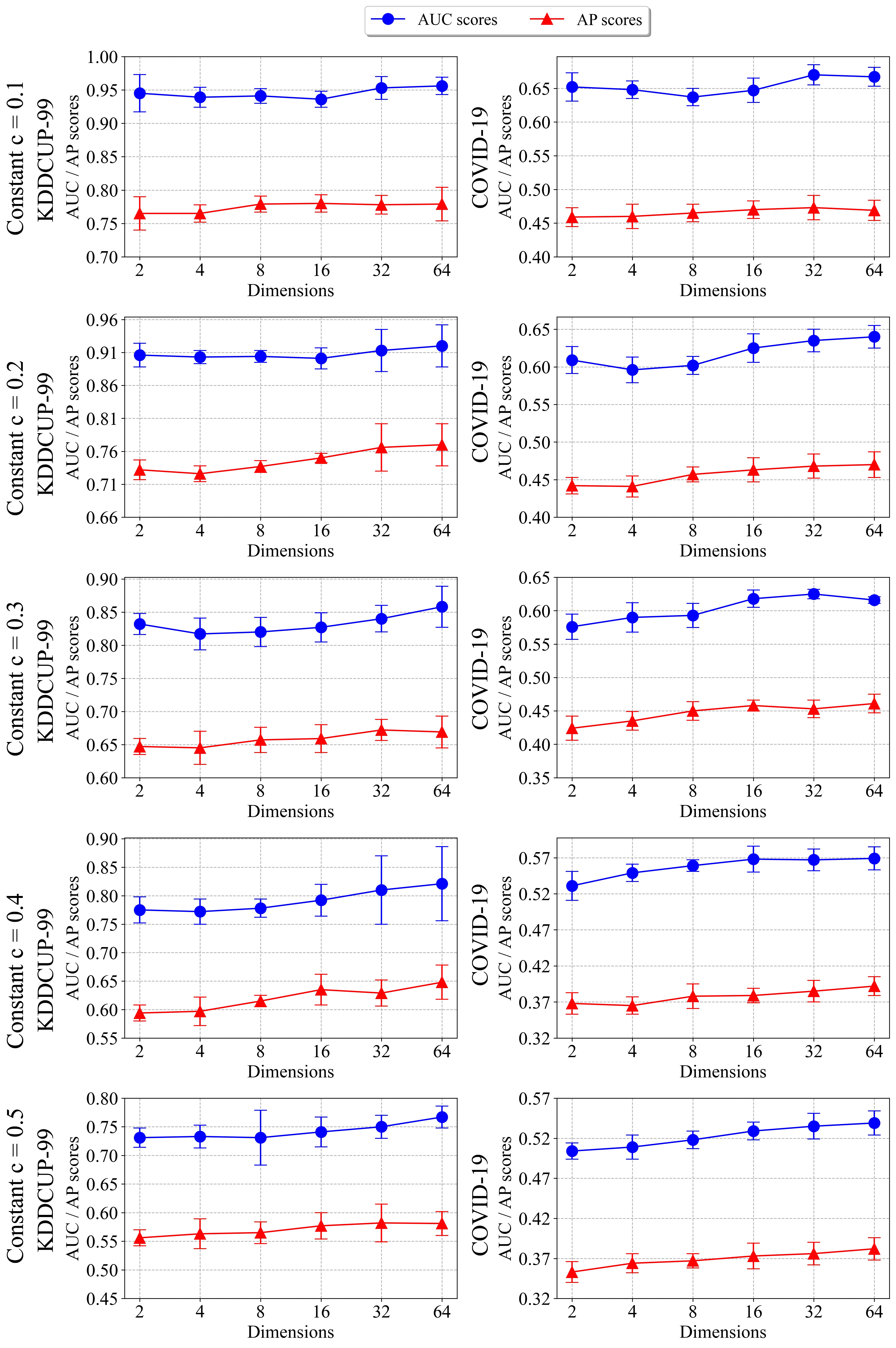
Our default value of the intrinsic dimension is . Here we study the sensitivity of our numerical results to the following choices intrinsic dimensions: , , , , and , while using the KDDCUP-99 and COVID-19 datasets. The training ratio of outliers per inliers are in . We compute the AUC and AP scores averaged over the testing ratios of outliers per inliers, , , , and , and over three runs of the same setting. Fig. 5 reports the averaged results and their standard deviations, which are indicated by error bars.
.
We can see that larger intrinsic dimensions generally result in better performances. However, the improvement is not significant and not consistent for smaller dimensions. Furthermore, higher dimensions require more substantial computational efforts for training.
B.2 Sensitivity to the Mixture Parameter
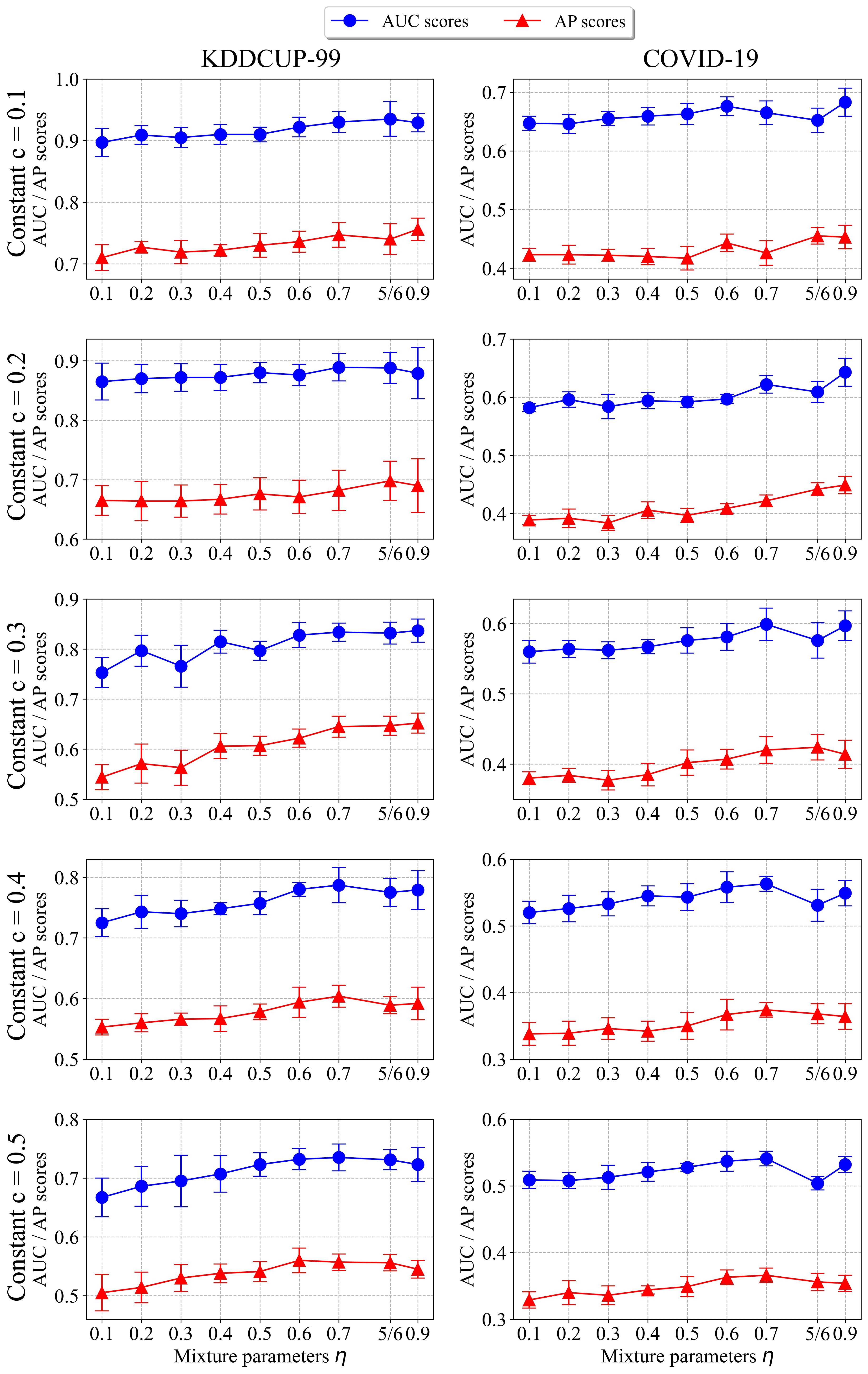
The default value of the mixture parameter is . Here we study the sensitivity of the accuracy of MAW to the mixture parameters: . We use , instead of the nearby value 0.8, since it was already tested for MAW. The training ratios of outliers per inliers are , , , and . Following the same procedure of §B, we average the AUC and AP scores for both KDDCUP-99 and COVID-19. We report them in Fig. 6.
We notice that the AUC and AP scores mildly increase as increases (though they may slightly decrease at 0.9). It seems that MAW learns well the inlier mode with a sufficiently large inlier weight, where the variation in the accuracy as a function of is not large in general.
Appendix C RUNTIME COMPARISON
Table 1 summarizes runtimes of all the above experiments with . The initially computed runtimes are times measured for completing single experiments with a single epoch. The table averages each such runtime over the different classes and different outlier ratios for testing. We note that LOF, OCSVM and IF are faster than the rest of the methods since they do not require training neural networks. Among the neural-networks-based methods, RSRAE is the fastest and OCGAN, DAGMM and MAW are the slowest. Indeed, RSRAE has a single autoencoder and OCGAN, DAGMM and MAW contain several neural networks. Another possible reason for the relative slowness of MAW is due to its dimension reduction component, whose implementation in TensorFlow seems to be computationally expensive. However, it seems to help achieve competitive performance in detecting outliers. We plan to investigate a more efficient implementation of the dimension reduction component in the future.
| Methods | COVID-19 | CIFAR-10 | Caltech101 | Fashion MNIST | KDDCUP-99 | Reuters-21578 |
|---|---|---|---|---|---|---|
| LOF | 0.30 0.17 | 3.98 0.13 | 0.24 0.01 | 16.31 1.01 | 3.23 0.04 | 17.91 1.98 |
| OCSVM | 0.17 0.07 | 2.22 0.09 | 0.12 0.00 | 8.34 2.36 | 9.08 0.05 | 8.74 1.47 |
| IF | 0.43 0.01 | 1.86 0.12 | 0.39 0.01 | 2.86 0.37 | 1.67 0.03 | 10.54 1.89 |
| RSRAE | 4.31 0.45 | 8.49 0.77 | 5.69 0.36 | 23.69 0.39 | 40.18 0.33 | 6.22 0.25 |
| DSEBMs | 48.30 3.45 | 66.57 2.35 | 147.15 0.32 | 151.02 7.67 | 216.02 4.34 | 74.28 2.09 |
| OCGAN | 182.79 2.53 | 313.28 0.13 | 679.44 4.62 | 250.51 0.24 | 2035.83 8.34 | 343.02 7.42 |
| DAGMM | 99.44 5.76 | 134.36 9.12 | 504.11 11.31 | 353.65 14.57 | 396.44 7.65 | 177.30 3.56 |
| MAW | 136.42 0.16 | 1871.22 16.03 | 217.32 0.25 | 1441.97 15.123 | 3166.62 12.12 | 255.85 2.97 |
Appendix D EXPERIMENTS WITH DIFFERENT TYPES OF OUTLIERS
In this section, we test the performance of MAW and the benchmark methods when the training and test sets are corrupted by outliers with different structures. We generate a dataset, which we call “Mix Caltech101”, in the following way. We fix the largest class of Caltech101 (containing airplane images) as the inlier class and randomly split it into the training inlier class (68.75) and testing inlier class (31.25). We form the training set by corrupting the training inlier class with random samples from the ten classes of CIFAR-10 (Krizhevsky 2009) with training ratio of outliers per inliers . For the test set, we corrupt the testing inlier class by “tile images” from MVTech dataset (Bergmann et al. 2019) with testing ratio of outliers per inliers in . The rest of the settings of the experiments are identical to the description in §4.2 of the main text. We present the AUC and AP scores and their standard deviations in Fig. 7.

Clearly, the competitive advantage of MAW is also noticeable in this setting. We note that OCSVM, the traditional distance-based method, and IF, the traditional density-based method, perform poorly in this scenario, whereas they performed well in our original setting.
Appendix E ADDITIONAL THEORETICAL GUARANTEES FOR THE MINIMIZATION
In §E.1 we fully motivate our focus on studying (12) in order to understand the advantage of the use of the Wasserstein distance over the KL divergence in the framework of MAW. In §E.2 we prove Proposition 3.1. In §E.3, we discuss a possible deviation of the clean theory of Proposition 3.2 from practice. In §E.4 we prove Proposition 3.2 and in §E.5 we prove Proposition 3.3.
E.1 Motivation for Studying (12)
The implementation of any VAE or its variants, such as AAE, WAE and MAW, requires the optimization of a regularization penalty , which measures the discrepancy between the latent and prior distributions. This penalty is typically the KL divergence, though one may use appropriate metrics such as or . Thus one needs to minimize
| (13) |
over the variational family indexed by some parameters. Here is the batch size of the input data and is its observed aggregated distribution.
Since the explicit expressions of the regularization measurements between aggregated distributions are unknown, it is not feasible to study the minimizer of (13). We thus consider the following approximation of (13):
| (14) |
We can minimize one term of this sum at a time, that, is minimize over . This minimization strategy is common in the study of the Wasserstein barycenter problem (Agueh & Carlier 2011; Peyré & Cuturi 2019; Chen et al. 2018).
One of the underlying assumptions of MAW is that the prior distribution is Gaussian and is a Gaussian mixture. That is, and . This gives rise to the following minimization problem
| (15) |
Similarly to approximating (13) by (14), we approximate (15) by (12). We remark that in (12) we further assume that there is a sufficiently small threshold for which . This is a reasonable assumption since, in practice, if and are very close, the reconstruction loss will be large.
E.2 Proof of Proposition 3.1
Recall that is the mean of the prior Gaussian, is the fixed separation parameter for the means of the two modes and is the fixed mixture parameter. For , 1, 2, we denote the Gaussian probability distribution by . Since in our setting , we denote the common covariance matrix in by . That is, for .
The case : We follow the next three steps to prove that the minimizer of (12) satisfies .
Step I: We prove that
| (16) |
First, we note that using the definition of and the common notation for the distribution on with marginals and
| (17) |
where the inequality follows from the fact that is convex and from Jensen’s inequality.
On the other hand, for or , let be an arbitrary random vector with distribution , and let . The distribution of is Gaussian with mean and covariance , that is, this distribution is . Let be the joint distribution of the random variables and . We note that is in and that
Therefore,
| (18) |
Step II: We prove that (12) with , , is equivalent to
| (19) |
We first note that (12) with , is equivalent to
| (20) |
Indeed, this is a direct consequence of the expression derived in step I for in this case. It is thus left to show that if , minimize (20), then we can construct , that are colinear with and also minimize (20).
For any and in with and for the given , we define , and and demonstrate them in Fig. 8. The point is the projection of onto and for , . We observe the following properties, which can be proved by direct calculation, though Fig. 8 also clarifies them:
and consequently,
| (21) |
| (22) |
and
| (23) |
Clearly, the combination of (21), (22) and (23) concludes the proof of step II. That is, it implies that if , minimize (20), then and defined above are colinear with and also minimize (20).

Step III: We directly solve (19) and consequently (12) with , . Due to the colinearity constraint in (12), we can write
| (24) |
The objective function in (19) can then be written as
where equality is achieved if and only if . We thus define and note that
and its derivative is
The above expressions for and and the assumption that imply that is increasing when , decreasing when and . Thus has a global minimum at . Hence, it follows from (24) that the minimizer of (12), and equivalently (12) with , satisfies .
The case : We prove that the solution of (12) with satisfies . We practically follow similar steps as the proof above.
Step I: We derive an expression for , where , 2. We use the following general formula, which holds for the case where , and are general covariance matrices in (see e.g., (2) in (Hershey & Olsen 2007)):
| (25) |
Since in our setting , this expression has the simpler form:
Step II: We reformulate the optimization problem. The above step implies that (12) with can be written as
or equivalently,
| (26) |
We express the eigenvalue decomposition of as , where , and is an orthogonal matrix. Applying the change of variables for , 1, 2, we rewrite (26) as
| (27) |
At last, applying the same colinearity argument as above (supported by Fig. 8) we conclude the following equivalent formulation of (27):
| (28) |
E.3 Some Remarks on Proposition 3.2
We clarify why the statement and proof of the proposition are not sufficient for explaining the effect of the optimization on MAW. We note that the inlier and outlier covariances, and , obtained by Proposition 3.2, are diagonal. Furthermore, the proof of Proposition 3.2 clarifies that the underlying minimization problem of this proposition may assume without loss of generality that the inlier and outlier covariances are diagonal (see e.g., (31)). On the other hand, the numerical results in §4.3 of the main text support the use of full covariances, instead of diagonal covariance. Nonetheless, we claim that the full covariances of MAW come naturally from the dimension reduction component of MAW. This component also contains trainable parameters for the covariances and they will affect the weights of the encoder, that is, will affect both the minimization and the reconstruction loss. Thus the analysis of the minimization component is not sufficient for inferring the whole behavior of MAW. For tractability purposes, the minimization in (12) ignores the dimension reduction component. For completeness we remark that there are two other differences between the use of (12) in Proposition 3.2 and the way it arises in MAW that may possibly also result in the advantage of using full covariance in MAW. First of all, the minimization in Proposition 3.2 uses , whereas MAW uses , which we find intractable when using the rest of the setting of Proposition 3.2. Second of all, (12) with is an approximation of the minimization of (see §E.1 for explanation), which is also intractable (even if one uses ).
E.4 Proof of Proposition 3.2
We follow the same steps of the proof of Proposition 3.1.
Step I: We immediately verify the formula
| (30) |
We use the following general formula, which holds for the case where , and are general covariance matrices in (see e.g., (4) in (Panaretos & Zemel 2019)): For ,
Indeed, (30) is obtained as a direct consequence of (E.4) using the identity
Step II: We reformulate the underlying minimization problem in two different stages. We first claim that the minimizer of (12) with and the constraint that is of rank and is of rank can be expressed as the minimizer of
| (31) |
In view of (12) and (30) we only need to prove that the minimizer of (31) is the same if one removes the constraint that and are both diagonal matrices and require instead that they are in . This is easy to show. Indeed, if for or , , then it can be diagonalized as follows: , where is diagonal and is orthogonal. Hence, and
Consequently,
and the above claim is concluded.
Next, we vectorize the minimization problem in (31) as follows. We denote by the set of positive real numbers. Let be a general vector in , be a general vector in and . Given, the constraints on and , we can parametrize the diagonal elements of and by and , that is, we set diag() and diag(). The objective function of (31) can then be written as
Combining this last expression and the same colinearity argument as in the proof of Proposition 3.1 in §E.2 (supported by Fig. 8), (31) is equivalent to
| (32) |
Step III: We solve (32). By the colinearity constraint, we can write , where . We thus obtain that
| (33) |
Furthermore, denoting the coordinates of and by and , we similarly obtain that
| (34) |
The last two of equations imply that
and
Combining (30), (33) and the above two equations, we rewrite the objective function of (32) as follows:
| (35) |
where equality is achieved if and only if . One can make the following two observations: does not yield a minimizer of (32), and for any , (35) obtains its minimum at . In view of these observations and the derivation above, we define
| (36) |
and note that (32) is equivalent to
| (37) |
We rewrite as
We denote
and
Their derivatives are
and
These expressions for and imply that the critical points for are
and the critical points for are
We note that is increasing on and decreasing on . On the other hand, is increasing on and decreasing on . Since , . The derivative of with respect to is
So is increasing on and decreasing on . The values of at and are
Consequently, the minimum of is obtained at . By (33) and (34), the means , and the covariance matrices , satisfy: , and . Moreover, the norms of and can be computed from (34) as and , respectively.
E.5 Proof of Proposition 3.3
Notice that since , det. On the other hand, since with rank, det. Therefore,
This and (25) imply that .
Appendix F ADDITIONAL DETAILS ON THE BENCHMARK METHODS
We overview the benchmark methods compared with MAW, where we present them according to alphabetical order of names. We will include all tested codes in a supplemental webpage.
For completeness, we mention the following links (or papers with links) we used for the different codes. For DSEBMs and DAGMM we used the codes of (Golan & El-Yaniv 2018). For LOF, OCSVM and IF we used the scikit-learn (Buitinck et al. 2013) packages for novelty detection. For OCGAN we used its TensorFlow implementation from https://pypi.org/project/ocgan. For RSRAE, we adapted the code of (Lai et al. 2020) to novelty detection.
All experiments were executed on a Linux machine with 64GB RAM and four GTX1080Ti GPUs.
We remark that for the neural networks based methods (DAGMM, DSEBMs, OCGAN and RSRAE), we followed similar implementation details as the one described in §A.3 for MAW.
Deep Autoencoding GMM (DAGMM) (Zong et al. 2018): This method uses a deep autoencoder model. It optimizes an end-to-end structure that contains both an autoencoder and an estimator for a GMM. Anomalies are detected using this GMM. We remark that this mixture model is proposed for the inliers. An improved version of DAGMM was recently proposed in (Fan et al. 2020).
Deep Structured Energy-Based Models (DSEBMs) (Zhai et al. 2016): Its decision is based on an energy function which is the negative log probability that a sample follows the data distribution. An autoencoder is used for the energy-based model in order to avoid the need of complex sampling.
Isolation Forest (IF) (Liu et al. 2008): It iteratively constructs special binary trees for the training set and identifies anomalies in the test set as the ones with shortest average path lengths.
Local Outlier Factor (LOF) (Breunig et al. 2000): It measures the isolation of a data point from its surrounding neighbors by estimating the local density of this point using its nearest neighbors. In novelty detection, it identifies novelties according to low density regions learned from the training data.
One-class Novelty Detection Using GANs (OCGAN) (Perera et al. 2019): It is composed of four NNs: a denoising autoencoder, two adversarial discriminators, and a classifier. It adversarially encourages the autoencoder to learn only the inlier features.
One-Class SVM (OCSVM) (Heller et al. 2003): It estimates the margin of the training set and uses it as the decision boundary for the test set. It commonly utilizes a radial basis function kernel.
Robust Subspace Recovery Autoencoder (RSRAE) (Lai et al. 2020): It uses an autoencoder with a linear RSR layer and an -based penalty. The RSR layer extracts features of inliers in the latent code while helping to reject outliers. The instances with higher reconstruction errors are viewed as outliers. RSRAE trains a model using the training data. We then apply this model for detecting novelties in the test data.
Appendix G ADDITIONAL DETAILS ON THE DIFFERENT DATASETS
Below we provide additional details on the six datasets used in our experiments. We remark that each dataset contains several clusters (3 for COVID-19, 10 for CIFAR-10, 11 largest ones for Caltech101, 10 for Fashion MNIST, 2 for KDDCUP-99 and 5 for Reuters-21578, ). Table 2 lists for each dataset (for both training and testing) the data types, numbers of clusters, dimensions, numbers of instances and numbers of inliers and outliers.
| Dataset information | Training | Testing | |||||||||
|---|---|---|---|---|---|---|---|---|---|---|---|
| Datasets | Type | Clusters | Dimension | Instances | Inliers | Outliers | Inliers | Outliers | |||
| COVID-19 (Radiography) | Image | 3 | 15,161 | 160 | 160 | 60 | 60 | ||||
| CIFAR-10 | Image | 10 | 60,000 | 450 | 450 | 150 | 150 | ||||
| Caltech101 | Image | 11 | 9,146 | 100 | 100 | 100 | 100 | ||||
| Fashion MNIST | Image | 10 | 70,000 | 300 | 300 | 60 | 60 | ||||
| KDDCUP-99 | Feature | 2 | 494,021 | 6000 | 6000 | 1200 | 1200 | ||||
| Reuters-21578 | Feature | 5 | 21,578 | 350 | 350 | 140 | 140 | ||||
COVID-19 (Radiography) (Chowdhury et al. 2020): It contains chest X-ray images (RGB) labeled according to these categories: COVID-19 positive, normal and bacterial Pneumonia cases. We resize the images to size and rescale the pixel intensities to lie in . It is publicly available in https://www.kaggle.com/tawsifurrahman/covid19-radiography-database.
CIFAR-10 (Krizhevsky 2009): It contains 10 categories of RGB images of transportation vehicles and animals. We rescale the pixel intensities to lie in . The dataset is publicly available in https://www.cs.toronto.edu/~kriz/cifar.html.
Caltech101 (Fei-Fei et al. 2004): It contains RGB images of objects from 101 categories with identifying labels. Following Lai et al. 2020, we use the largest 11 classes and preprocess their images to have size and rescale the pixel intensities to lie in . It is publicly available in http://www.vision.caltech.edu/Image_Datasets/Caltech101.
Fashion MNIST (Xiao et al. 2017): It is an image dataset containing 10 categories of grayscale images of clothing and accessories items. We rescaled the pixel intensities to lie in . We obtained the dataset from the Keras dataset library https://keras.io/api/datasets/fashion_mnist.
KDDCUP-99 (Dua & Graff 2017): It is a classic dataset for intrusion detection. It contains feature vectors of connections between internet protocols and a binary label for each feature vector identifying normal vs. abnormal ones. The abnormal ones are associated with an “attack” or “intrusion”. The dataset is publicly available in http://kdd.ics.uci.edu/databases/kddcup99/kddcup99.html.
Reuters-21578 (Lewis 1997): It contains 21,578 documents with 90 text categories having multi-labels. Following Lai et al. 2020, we consider the five largest classes with single labels. We utilize the scikit-learn packages: TFIDF and HashingVectorizer (Rajaraman & Ullman 2011) to preprocess the documents into 26,147 dimensional vectors. It is publicly available in https://archive.ics.uci.edu/ml/datasets/reuters-21578+text+categorization+collection.
According to the above description, the numbers of clusters of these datasets are 3, 10, 11, 10, 2 and 5, respectively. We remark that COVID-19, CIFAR-10, Caltech101, Fashion MNIST and Reuters-21578 separate between training and testing data points. For KDDCUP-99, we randomly split it into training and testing datasets of equal sizes.
Appendix H NUMERICAL RESULTS OF THE EXPERIMENTS
We present as tables the numerical values depicted in Figs. 2 and 3. Tables 3-14 report the averaged AUC and AP scores with training outliers/inliers ratio that were depicted in Fig. 2. Each table describes one of the averaged scores (AUC or AP) for one of the six datasets (COVID-19, CIFAR-10, Caltech101, Fashion MNIST, KDDCUP-99 and Reuters-21578) and also indicates the standard deviation of each value. The outperforming methods are marked in bold.
Tables 15-18 record the averaged AUC and AP scores with training outliers/inliers ratio that were depicted in Fig. 3. Each table describes one of the averaged scores (AUC or AP) for one of either KDDCUP-99 or COVID-19 and also indicates the standard deviation of each value. The outperforming methods are boldfaced.
| Training ratio of outliers per inliers, | |||||
|---|---|---|---|---|---|
| Methods | 0.1 | 0.2 | 0.3 | 0.4 | 0.5 |
| MAW | 0.652 0.021 | 0.609 0.018 | 0.576 0.019 | 0.531 0.020 | 0.504 0.010 |
| DAGMM | 0.527 0.068 | 0.545 0.051 | 0.518 0.062 | 0.504 0.060 | 0.503 0.057 |
| DSEBMs | 0.451 0.000 | 0.451 0.000 | 0.451 0.000 | 0.451 0.000 | 0.451 0.000 |
| IF | 0.574 | 0.541 | 0.515 | 0.493 | 0.469 |
| LOF | 0.642 | 0.588 | 0.542 | 0.536 | 0.519 |
| OCGAN | 0.472 0.000 | 0.472 0.000 | 0.465 0.000 | 0.445 0.000 | 0.431 0.000 |
| OCSVM | 0.528 | 0.528 | 0.528 | 0.535 | 0.521 |
| RSRAE | 0.535 0.031 | 0.507 0.028 | 0.456 0.023 | 0.434 0.018 | 0.407 0.011 |
| Training ratio of outliers per inliers, | |||||
|---|---|---|---|---|---|
| Methods | 0.1 | 0.2 | 0.3 | 0.4 | 0.5 |
| MAW | 0.459 0.014 | 0.442 0.011 | 0.424 0.018 | 0.368 0.015 | 0.353 0.013 |
| DAGMM | 0.354 0.053 | 0.390 0.057 | 0.316 0.052 | 0.357 0.050 | 0.348 0.047 |
| DSEBMs | 0.372 0.000 | 0.375 0.000 | 0.364 0.000 | 0.360 0.000 | 0.358 0.000 |
| IF | 0.425 | 0.404 | 0.392 | 0.373 | 0.363 |
| LOF | 0.463 | 0.422 | 0.402 | 0.374 | 0.371 |
| OCGAN | 0.381 0.000 | 0.381 0.000 | 0.381 0.000 | 0.373 0.000 | 0.350 0.000 |
| OCSVM | 0.315 | 0.315 | 0.315 | 0.372 | 0.365 |
| RSRAE | 0.388 0.018 | 0.377 0.016 | 0.355 0.011 | 0.352 0.010 | 0.340 0.009 |
| Training ratio of outliers per inliers, | |||||
|---|---|---|---|---|---|
| Methods | 0.1 | 0.2 | 0.3 | 0.4 | 0.5 |
| MAW | 0.621 0.013 | 0.609 0.014 | 0.607 0.012 | 0.600 0.010 | 0.595 0.013 |
| LOF | 0.582 | 0.574 | 0.559 | 0.551 | 0.539 |
| OCSVM | 0.595 | 0.587 | 0.580 | 0.564 | 0.570 |
| IF | 0.603 | 0.586 | 0.596 | 0.581 | 0.569 |
| RSRAE | 0.638 0.010 | 0.607 0.017 | 0.599 0.023 | 0.610 0.025 | 0.589 0.023 |
| DSEBMs | 0.586 0.006 | 0.584 0.006 | 0.580 0.004 | 0.576 0.006 | 0.556 0.006 |
| OCGAN | 0.501 0 | 0.501 0 | 0.499 0 | 0.487 0 | 0.476 0 |
| DAGMM | 0.574 0.030 | 0.557 0.035 | 0.541 0.037 | 0.510 0.0331 | 0.545 0.037 |
| Training ratio of outliers per inliers, | |||||
|---|---|---|---|---|---|
| Methods | 0.1 | 0.2 | 0.3 | 0.4 | 0.5 |
| MAW | 0.427 0.010 | 0.419 0.012 | 0.414 0.011 | 0.4000.009 | 0.411 0.011 |
| LOF | 0.395 | 0.036 | 0.377 | 0.374 | 0.371 |
| OCSVM | 0.408 | 0.400 | 0.393 | 0.378 | 0.385 |
| IF | 0.416 | 0.395 | 0.403 | 0.389 | 0.373 |
| RSRAE | 0.434 0.011 | 0.412 0.020 | 0.417 0.022 | 0.391 0.019 | 0.400 0.014 |
| DSEBMs | 0.391 0.008 | 0.388 0.008 | 0.386 0.004 | 0.382 0.006 | 0.3790.003 |
| OCGAN | 0.342 0 | 0.3400 | 0.339 0 | 0.337 0 | 0.3350 |
| DAGMM | 0.378 0.049 | 0.369 0.041 | 0.355 0.030 | 0.308 0.026 | 0.352 0.047 |
| Training ratio of outliers per inliers, | |||||
|---|---|---|---|---|---|
| Methods | 0.1 | 0.2 | 0.3 | 0.4 | 0.5 |
| MAW | 0.801 0.017 | 0.760 0.028 | 0.700 0.038 | 0.608 0.031 | 0.570 0.021 |
| DAGMM | 0.684 0.100 | 0.588 0.115 | 0.500 0.100 | 0.509 0.101 | 0.514 0.095 |
| DSEBMs | 0.536 0.011 | 0.612 0.025 | 0.577 0.030 | 0.564 0.021 | 0.536 0.021 |
| IF | 0.755 | 0.694 | 0.626 | 0.575 | 0.540 |
| LOF | 0.674 | 0.593 | 0.495 | 0.436 | 0.411 |
| OCGAN | 0.494 0.000 | 0.494 0.000 | 0.494 0.000 | 0.500 0.000 | 0.500 0.000 |
| OCSVM | 0.682 | 0.618 | 0.577 | 0.538 | 0.516 |
| RSRAE | 0.774 0.027 | 0.722 0.041 | 0.664 0.082 | 0.579 0.047 | 0.568 0.036 |
| Training ratio of outliers per inliers, | |||||
|---|---|---|---|---|---|
| Methods | 0.1 | 0.2 | 0.3 | 0.4 | 0.5 |
| MAW | 0.634 0.027 | 0.572 0.039 | 0.531 0.064 | 0.412 0.029 | 0.414 0.021 |
| DAGMM | 0.574 0.088 | 0.422 0.112 | 0.308 0.102 | 0.351 0.074 | 0.363 0.076 |
| DSEBMs | 0.385 0.003 | 0.472 0.051 | 0.3980.019 | 0.383 0.023 | 0.365 0.028 |
| IF | 0.545 | 0.486 | 0.430 | 0.304 | 0.371 |
| LOF | 0.460 | 0.400 | 0.337 | 0.304 | 0.290 |
| OCGAN | 0.362 0.000 | 0.362 0.000 | 0.362 0.000 | 0.362 0.000 | 0.362 0.000 |
| OCSVM | 0.472 | 0.419 | 0.380 | 0.352 | 0.339 |
| RSRAE | 0.595 0.038 | 0.551 0.045 | 0.495 0.073 | 0.425 0.040 | 0.443 0.027 |
| Training ratio of outliers per inliers, | |||||
|---|---|---|---|---|---|
| Methods | 0.1 | 0.2 | 0.3 | 0.4 | 0.5 |
| MAW | 0.897 0.013 | 0.879 0.011 | 0.852 0.022 | 0.830 0.017 | 0.801 0.016 |
| DAGMM | 0.607 0.093 | 0.376 0.070 | 0.427 0.090 | 0.401 0.078 | 0.411 0.081 |
| DSEBMs | 0.730 0.092 | 0.729 0.105 | 0.739 0.086 | 0.723 0.106 | 0.687 0.096 |
| IF | 0.893 | 0.875 | 0.843 | 0.834 | 0.827 |
| LOF | 0.569 | 0.507 | 0.476 | 0.468 | 0.458 |
| OCGAN | 0.542 0.006 | 0.538 0.004 | 0.544 0.014 | 0.531 0.003 | 0.525 0.004 |
| OCSVM | 0.895 | 0.874 | 0.848 | 0.831 | 0.814 |
| RSRAE | 0.860 0.022 | 0.848 0.022 | 0.829 0.042 | 0.831 0.028 | 0.808 0.028 |
| Training ratio of outliers per inliers, | |||||
|---|---|---|---|---|---|
| Methods | 0.1 | 0.2 | 0.3 | 0.4 | 0.5 |
| MAW | 0.788 0.013 | 0.754 0.014 | 0.7230.029 | 0.686 0.025 | 0.672 0.021 |
| DAGMM | 0.482 0.051 | 0.303 0.057 | 0.334 0.113 | 0.318 0.056 | 0.330 0.038 |
| DSEBMs | 0.600 0.045 | 0.609 0.120 | 0.6130.089 | 0.605 0.086 | 0.565 0.072 |
| IF | 0.768 | 0.724 | 0.693 | 0.665 | 0.642 |
| LOF | 0.382 | 0.331 | 0.308 | 0.301 | 0.294 |
| OCGAN | 0.504 0.002 | 0.503 0.003 | 0.500 0.059 | 0.495 0.001 | 0.493 0.001 |
| OCSVM | 0.801 | 0.768 | 0.735 | 0.696 | 0.664 |
| RSRAE | 0.749 0.029 | 0.736 0.032 | 0.716 0.048 | 0.683 0.036 | 0.680 0.042 |
| Training ratio of outliers per inliers, | |||||
|---|---|---|---|---|---|
| Methods | 0.1 | 0.2 | 0.3 | 0.4 | 0.5 |
| MAW | 0.945 0.028 | 0.906 0.018 | 0.832 0.016 | 0.775 0.023 | 0.731 0.017 |
| DAGMM | 0.614 0.083 | 0.660 0.109 | 0.584 0.133 | 0.457 0.099 | 0.521 0.089 |
| DSEBMs | 0.514 0.000 | 0.499 0.000 | 0.497 0.000 | 0.496 0.000 | 0.496 0.000 |
| IF | 0.811 | 0.850 | 0.807 | 0.750 | 0.706 |
| LOF | 0.480 | 0.527 | 0.516 | 0.527 | 0.530 |
| OCGAN | 0.651 0.157 | 0.552 0.157 | 0.617 0.191 | 0.517 0.146 | 0.628 0.155 |
| OCSVM | 0.502 | 0.568 | 0.567 | 0.555 | 0.534 |
| RSRAE | 0.815 0.031 | 0.839 0.059 | 0.774 0.086 | 0.735 0.066 | 0.710 0.056 |
| Training ratio of outliers per inliers, | |||||
|---|---|---|---|---|---|
| Methods | 0.1 | 0.2 | 0.3 | 0.4 | 0.5 |
| MAW | 0.765 0.025 | 0.732 0.015 | 0.647 0.012 | 0.594 0.014 | 0.556 0.014 |
| DAGMM | 0.446 0.047 | 0.506 0.064 | 0.459 0.087 | 0.373 0.109 | 0.464 0.998 |
| DSEBMs | 0.450 0.000 | 0.447 0.000 | 0.446 0.000 | 0.444 0.000 | 0.444 0.000 |
| IF | 0.636 | 0.6331 | 0.562 | 0.493 | 0.457 |
| LOF | 0.391 | 0.407 | 0.392 | 0.394 | 0.391 |
| OCGAN | 0.582 0.132 | 0.472 0.163 | 0.525 0.133 | 0.418 0.136 | 0.535 0.133 |
| OCSVM | 0.543 | 0.598 | 0.595 | 0.438 | 0.426 |
| RSRAE | 0.704 0.048 | 0.698 0.050 | 0.606 0.065 | 0.584 0.034 | 0.574 0.046 |
| Training ratio of outliers per inliers, | |||||
|---|---|---|---|---|---|
| Methods | 0.1 | 0.2 | 0.3 | 0.4 | 0.5 |
| MAW | 0.885 0.028 | 0.830 0.013 | 0.770 0.017 | 0.700 0.002 | 0.648 0.016 |
| DAGMM | 0.500 0.000 | 0.511 0.027 | 0.566 0.110 | 0.559 0.087 | 0.570 0.091 |
| DSEBMs | 0.887 0.012 | 0.825 0.012 | 0.790 0.015 | 0.690 0.002 | 0.648 0.010 |
| IF | 0.544 | 0.535 | 0.520 | 0.453 | 0.452 |
| LOF | 0.757 | 0.612 | 0.579 | 0.631 | 0.616 |
| OCGAN | 0.648 0.127 | 0.477 0.129 | 0.498 0.140 | 0.519 0.132 | 0.502 0.099 |
| OCSVM | 0.882 | 0.817 | 0.785 | 0.673 | 0.640 |
| RSRAE | 0.786 0.042 | 0.755 0.034 | 0.716 0.033 | 0.605 0.001 | 0.494 0.004 |
| Training ratio of outliers per inliers, | |||||
|---|---|---|---|---|---|
| Methods | 0.1 | 0.2 | 0.3 | 0.4 | 0.5 |
| MAW | 0.755 0.041 | 0.677 0.026 | 0.627 0.029 | 0.518 0.004 | 0.474 0.013 |
| DAGMM | 0.316 0.000 | 0.316 0.013 | 0.365 0.020 | 0.362 0.015 | 0.372 0.012 |
| DSEBMs | 0.763 0.012 | 0.697 0.011 | 0.666 0.007 | 0.515 0.003 | 0.473 0.003 |
| IF | 0.368 | 0.372 | 0.365 | 0.301 | 0.298 |
| LOF | 0.580 | 0.438 | 0.421 | 0.498 | 0.486 |
| OCGAN | 0.408 0.045 | 0.334 0.098 | 0.365 0.106 | 0.504 0.083 | 0.497 0.094 |
| OCSVM | 0.746 | 0.681 | 0.637 | 0.467 | 0.438 |
| RSRAE | 0.593 0.051 | 0.563 0.035 | 0.488 0.036 | 0.403 0.001 | 0.415 0.003 |
| Training ratio of outliers per inliers, | |||||
|---|---|---|---|---|---|
| Methods | 0.1 | 0.2 | 0.3 | 0.4 | 0.5 |
| MAW | 0.945 0.028 | 0.906 0.018 | 0.832 0.016 | 0.775 0.023 | 0.731 0.017 |
| MAW-MSE | 0.844 0.039 | 0.812 0.032 | 0.746 0.044 | 0.709 0.020 | 0.675 0.014 |
| MAW-KL divergence | 0.905 0.026 | 0.863 0.028 | 0.801 0.029 | 0.752 0.016 | 0.696 0.018 |
| MAW-same rank | 0.912 0.023 | 0.868 0.011 | 0.797 0.022 | 0.750 0.012 | 0.699 0.040 |
| MAW-single Gaussian | 0.914 0.016 | 0.862 0.021 | 0.796 0.013 | 0.751 0.040 | 0.701 0.045 |
| MAW-diagonal cov. | 0.918 0.023 | 0.858 0.020 | 0.801 0.044 | 0.743 0.017 | 0.703 0.015 |
| VAE | 0.821 0.048 | 0.785 0.027 | 0.732 0.046 | 0.717 0.018 | 0.685 0.027 |
| GMM prior | 0.677 0.009 | 0.6350.013 | 0.604 0.006 | 0.562 0.015 | 0.5170.014 |
| Training ratio of outliers per inliers, | |||||
|---|---|---|---|---|---|
| Methods | 0.1 | 0.2 | 0.3 | 0.4 | 0.5 |
| MAW | 0.765 0.025 | 0.732 0.015 | 0.647 0.012 | 0.594 0.014 | 0.556 0.014 |
| MAW-MSE | 0.715 0.079 | 0.589 0.058 | 0.524 0.053 | 0.4630.042 | 0.410 0.028 |
| MAW-KL divergence | 0.735 0.028 | 0.676 0.028 | 0.618 0.024 | 0.5790.023 | 0.5090.017 |
| MAW-same rank | 0.725 0.028 | 0.681 0.015 | 0.622 0.024 | 0.572 0.017 | 0.532 0.038 |
| MAW-single Gaussian | 0.737 0.018 | 0.675 0.023 | 0.620 0.025 | 0.5690.036 | 0.519 0.044 |
| MAW-diagonal cov. | 0.724 0.021 | 0.678 0.035 | 0.589 0.064 | 0.546 0.019 | 0.512 0.016 |
| VAE | 0.642 0.030 | 0.555 0.043 | 0.524 0.028 | 0.4780.024 | 0.4500.015 |
| GMM prior | 0.604 0.010 | 0.5870.013 | 0.557 0.009 | 0.534 0.011 | 0.5010.015 |
| Training ratio of outliers per inliers, | |||||
|---|---|---|---|---|---|
| Methods | 0.1 | 0.2 | 0.3 | 0.4 | 0.5 |
| MAW | 0.652 0.021 | 0.609 0.018 | 0.576 0.019 | 0.531 0.020 | 0.5040.010 |
| MAW-MSE | 0.602 0.022 | 0.554 0.063 | 0.528 0.041 | 0.507 0.014 | 0.4790.021 |
| MAW-KL divergence | 0.614 0.025 | 0.580 0.026 | 0.508 0.064 | 0.476 0.023 | 0.4630.016 |
| MAW-same rank | 0.604 0.031 | 0.574 0.048 | 0.527 0.044 | 0.430 0.017 | 0.4080.021 |
| MAW-single Gaussian | 0.621 0.027 | 0.5860.029 | 0.507 0.047 | 0.4920.021 | 0.4720.019 |
| MAW-diagonal cov. | 0.600 0.029 | 0.586 0.030 | 0.535 0.035 | 0.446 0.028 | 0.439 0.038 |
| VAE | 0.619 0.073 | 0.5650.065 | 0.522 0.049 | 0.508 0.023 | 0.4730.016 |
| GMM prior | 0.548 0.012 | 0.5140.008 | 0.489 0.010 | 0.476 0.011 | 0.4690.009 |
| Training ratio of outliers per inliers, | |||||
|---|---|---|---|---|---|
| Methods | 0.1 | 0.2 | 0.3 | 0.4 | 0.5 |
| MAW | 0.459 0.014 | 0.442 0.011 | 0.424 0.018 | 0.3680.015 | 0.3530.013 |
| MAW-MSE | 0.421 0.015 | 0.395 0.025 | 0.377 0.012 | 0.3320.013 | 0.328 0.020 |
| MAW-KL divergence | 0.427 0.016 | 0.403 0.012 | 0.370 0.021 | 0.3220.017 | 0.313 0.013 |
| MAW-same rank | 0.422 0.021 | 0.413 0.026 | 0.375 0.019 | 0.344 0.023 | 0.335 0.017 |
| MAW-single Gaussian | 0.425 0.019 | 0.409 0.012 | 0.374 0.016 | 0.339 0.014 | 0.3290.016 |
| MAW-diagonal cov. | 0.412 0.016 | 0.397 0.018 | 0.369 0.012 | 0.3430.009 | 0.330 0.009 |
| VAE | 0.412 0.030 | 0.411 0.043 | 0.379 0.028 | 0.3410.011 | 0.3330.013 |
| GMM prior | 0.389 0.009 | 0.3820.006 | 0.362 0.005 | 0.346 0.009 | 0.309 0.0096 |