EMNLP’21
Foreseeing the Benefits of Incidental Supervision
Abstract
Real-world applications often require improved models by leveraging a range of cheap incidental supervision signals. These could include partial labels, noisy labels, knowledge-based constraints, and cross-domain or cross-task annotations – all having statistical associations with gold annotations but not exactly the same. However, we currently lack a principled way to measure the benefits of these signals to a given target task, and the common practice of evaluating these benefits is through exhaustive experiments with various models and hyperparameters. This paper studies whether we can, in a single framework, quantify the benefits of various types of incidental signals for a given target task without going through combinatorial experiments. We propose a unified PAC-Bayesian motivated informativeness measure, PABI, that characterizes the uncertainty reduction provided by incidental supervision signals. We demonstrate PABI’s effectiveness by quantifying the value added by various types of incidental signals to sequence tagging tasks. Experiments on named entity recognition (NER) and question answering (QA) show that PABI’s predictions correlate well with learning performance, providing a promising way to determine, ahead of learning, which supervision signals would be beneficial.11 1 Our code is publicly available at https://github.com/CogComp/PABI.
1 Introduction
| Incidental Supervision Signals | Unified Measure | Support | |||||||
| Measures | partial | noisy | constraints | auxiliary | cross-domain | cross-type | mixed-type | Theoretical | Empirical |
| CST’11, HH’12, LD’14 | ✓ | ✓ | ✓ | ||||||
| AL’88, NDRT’13, RVBS’17 | ✓ | ✓ | ✓ | ||||||
| VW’17, WNR’20 | ✓ | ✓ | ✓ | ||||||
| NHFR’19 | ✓ | ✓ | ✓ | ||||||
| B’17 | ✓ | ✓ | |||||||
| GMSLBDS’20 | ✓ | ✓ | |||||||
| PABI (ours) | ✓ | ✓ | ✓ | ✓ | ✓ | ✓ | ✓ | ✓ | ✓ |
The supervised learning paradigm, where direct supervision signals are available in high-quality and large amounts, has been struggling to fulfill needs in many real-world AI applications. As a result, researchers and practitioners often resort to datasets that are not collected directly for the target task but capture some phenomena useful for it (Pan and Yang 2009; Vapnik and Vashist 2009; Roth 2017; Kolesnikov et al. 2019). However, it remains unclear how to predict the benefits of these incidental signals on our target task beforehand. For example, given two incidental signals that are relevant to the target task, it is still difficult for us to predict which one is more beneficial. Therefore, the common practice is often trial-and-error: perform experiments with different combinations of datasets and learning protocols, often exhaustively, to measure the impact on a target task (Liu et al. 2019; Khashabi et al. 2020). Not only is this very costly, but this trial-and-error approach can also be hard to interpret: if we don’t see improvements, is it because the incidental signals themselves are not useful for our target task, or is it because the learning protocols we have tried are inappropriate?
The difficulties of foreseeing the benefits of various incidental supervision signals, including partial labels, noisy labels, constraints22 2 Constraints are used to model dependencies among structured components in plenty of previous work such as CRF (Lafferty et al. 2001) and ILP (Roth and Yih 2004)., and cross-domain signals, are two-fold. First, it is hard to provide a unified measure because of the intrinsic differences among different signals (e.g., how do we predict and compare the benefit of learning from partial data and the benefit of knowing some constraints on the target task?). Second, it is hard to provide a practical measure supported by theory. Previous attempts are either not practical (Baxter 1998; Ben-David et al. 2010) or too heuristic (Gururangan et al. 2020), or apply to only one type of signals, e.g., noisy labels (Natarajan et al. 2013; Zhang et al. 2021). In this paper, we propose a unified PAC-Bayesian motivated informativeness measure (PABI) to quantify the value of incidental signals for sequence tagging tasks. We suggest that the informativeness of various incidental signals can be uniformly characterized by the uncertainty reduction they provide. Specifically, in the PAC-Bayesian framework, the informativeness is based on the Kullback–Leibler (KL) divergence between the prior and the posterior, where incidental signals are used to estimate a better prior (one that is closer to the gold posterior) to achieve better generalization performance. Furthermore, we provide a more practical entropy-based approximation of PABI. In practice, PABI first computes the entropy of the prior estimated from incidental signals, and then computes the relative decrease from the entropy of the prior without any information (i.e. the uniform prior) as the informativeness of incidental signals.
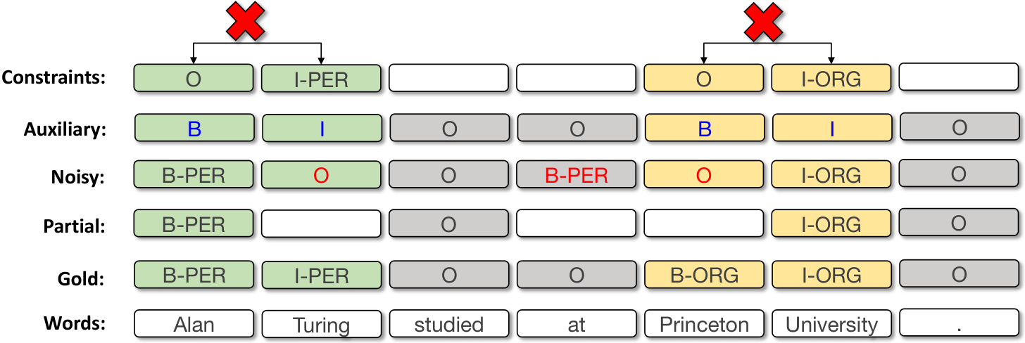
We have been in need of a unified informativeness measure like PABI. For instance, it might be obvious that we can expect better learning performance if the training data is less noisy and more completely annotated, but what if we want to compare the benefits of a noisy dataset to those of a dataset that is only partially labeled? PABI enables this kind of comparisons to be done analytically, without the need for experiments on a wide range of incidental signals such as partial labels, noisy labels, constraints, auxiliary labels (labels of another task), and cross-domain signals, for sequence tagging tasks in NLP. A specific example of NER is shown in Fig. 1, and the advantages of PABI can be found in Table 1.
Finally, our experiments on two NLP tasks, NER and QA, show that there is a strong positive correlation between PABI and the relative improvement for various incidental signals. This strong positive correlation indicates that the proposed unified, theory-motivated measure PABI can serve as a good indicator of the final learning performance, providing a promising way to know which signals are helpful for a target task beforehand.
2 Related Work
There are lots of practical measures proposed to quantify the benefits of specific types of signals. For example, a widely used measure for partial signals in structured learning is the partial rate (Cid-Sueiro 2012; Cour et al. 2011; Hovy and Hovy 2012; Liu and Dietterich 2014; Van Rooyen and Williamson 2017; Ning et al. 2019); a widely used measure for noisy signals is the noise ratio (Angluin and Laird 1988; Natarajan et al. 2013; Rolnick et al. 2017; Van Rooyen and Williamson 2017); Ning et al. 2019 propose to use the concaveness of the mutual information with different percentage of annotations to quantify the strength of constraints in the structured learning; others, in NLP, have quantified the contribution of constraints experimentally (Chang et al. 2008; Chang et al. 2012). Bjerva 2017 proposes to use conditional entropy or mutual information to quantify the value for auxiliary signals. As for domain adaptation, domain similarity can be measured by the performance gap between domains (Wang et al. 2019) or measures based on the language model in NLP, such as the vocabulary overlap (Gururangan et al. 2020). Among them, the most relevant work is Bjerva 2017. However, their conditional entropy or mutual information is based on token-level label distribution, which cannot be used for incidental signals involving multiple tokens or inputs, such as constraints and cross-domain signals. At the same time, for the cases where both PABI and mutual information can handle, PABI works similar to the mutual information as shown in Fig. 2, and PABI can further be shown to be a strictly increasing function of the mutual information. The key advantage of our proposed measure PABI is that PABI is a unified measure motivated by the PAC-Bayesian theory for a broader range of incidental signals compared to these practical measures for specific types of incidental signals.
There also has been a line of theoretical work that attempts to exploit incidental supervision signals. Among them, the most relevant part is task relatedness. Ben-David and Borbely 2008 define task relatedness based on the richness of transformations between inputs for different tasks, but their analysis is limited to cases where data is from the same classification problem but the inputs are in different subspace. Juba 2006 proposes to use the joint Kolmogorov complexity (Wallace and Dowe 1999) to characterize relatedness, but it is still unclear how to compute the joint Kolmogorov complexity in real-world applications. Mahmud and Ray 2008 further propose to use conditional Kolmogorov complexity to measure the task relatedness and provide empirical analysis for decision trees, but it is unclear how to use their relatedness for other models, such as deep neural networks. Thrun and O’Sullivan 1998 propose to cluster tasks based on the similarity between the task-optimal distance metric of k-nearest neighbors (KNN), but their analysis is based on KNN and it is unclear how to use their relatedness for other models. A lot of other works provide quite good qualitative analysis to show various incidental signals are helpful but they did not provide quantitative analysis to quantify to what extent these types of incidental signals can help (Abu-Mostafa 1993; Baxter 1998; Ben-David et al. 2010; Balcan and Blum 2010; Natarajan et al. 2013; London et al. 2016; Van Rooyen and Williamson 2017; Ciliberto et al. 2019; Wang et al. 2020). Compared to these theoretical analyses, PABI can be easily used in practice to quantify the benefits of a broader range of incidental signals.
3 PABI: A Unified PAC-Bayesian Informativeness Measure
We start with notations and preliminaries. Let be the input space, be the label space, and be the prediction space. Let denote the underlying distribution on . Let be the loss function that we use to evaluate learning algorithms. A set of training samples is generated i.i.d. from . In the common supervised learning setting, we usually assume the concept that generates data comes from the concept class . In this paper, we assume is finite, and its size is , which is common in sequence tagging tasks because of finite vocabulary and label set. We want to choose a predictor from such that it generalizes well to unseen data with respect to , measured by the generalization error . The training error over is .
More generally, instead of predicting a concept, we can specify a distribution over the concept class. Let denote the space of probability distributions over . General Bayesian learning algorithms (Zhang 2006) in the PAC-Bayesian framework (McAllester 1999a; McAllester 1999b; Seeger 2002; McAllester 2003b; McAllester 2003a; Maurer 2004; Guedj and Shawe-Taylor 2019) aim to choose a posterior over the concept class based on a prior and training data , where is a hyper parameter that controls the tradeoff between the prior and the data likelihood. In this setting, the training error and the generalization error need to be generalized, to take the distribution into account, as and respectively. When the posterior is one-hot (exactly one entry of the distribution is ), we have the original definitions of training error and generalization error, as in the PAC framework (Valiant 1984).
We are now ready to derive the proposed informativeness measure PABI motivated by PAC-Bayes. The generalization error bound in the PAC-Bayesian framework (Catoni 2007; Guedj and Shawe-Taylor 2019) says that with probability over , the following bound holds
where is the posterior distribution with the optimal , is the gold posterior that generates the data, denotes the KL divergence from to , and are two constants. This is based on the Theorem 2 in Guedj and Shawe-Taylor 2019.
As shown in the generalization bound, the generalization error is bounded by the KL divergence from the prior distribution to the gold posterior distribution. Therefore, we propose to utilize incidental signals to improve the prior distribution from to so that it is closer to the gold posterior distribution . Correspondingly, we can define PABI, the informativeness measure for incidental supervision signals, by measuring the improvement with regard to the gold posterior, in the KL divergence sense.
Definition 3.1 (PABI).
Suppose we use incidental signals to improve the prior distribution from to . The informativeness measure for incidental signals, PABI, is defined as
| (1) |
Remark. Note that if , while if , then . This result is consistent with our intuition that the closer is to , the more benefits we can gain from incidental signals. The square root function is used in PABI for two reasons: first, the generalization bounds in both PAC-Bayesian and PAC (see Appx. A.1) frameworks have the square root function; second, in our later experiments, we find that square root function can significantly improve the Pearson correlation between the relative performance improvement and PABI. It is worthwhile to note that the square root is not crucial for our framework, because our goal is to compare the benefits among different incidental supervision signals, where the relative values are expressive enough. In this sense, any strictly increasing function in over the current formulation would be acceptable.
We focus on the setting that the gold posterior is one-hot, which means concentrates on the true concept , though the definition of PABI can handle general gold posterior. However, is unknown in practice, which makes Eq. (1) hard to be computed in reality. In the following, we provide an approximation of PABI.
Definition 3.2 (Approximation of PABI).
Assume that the original prior is uniform, and the gold posterior is one-hot concentrated on the true concept in , as we have assumed that is finite. Let be the entropy function. The approximation of PABI is defined as
| (2) |
The uniform prior is usually used when we do not have information about the prior on which concept in the class that generates data. The intuition behind is that, it measures how much entropy incidental signals reduce, compared with non-informative prior . can be computed through data and thus is practical. To see how this approximation works, first note because is one-hot and is uniform over the finite concept class . Let be the one-hot distribution concentrated on concept for each . The approximation is that we estimate by , where follows : , and . Therefore,
As shown in Appx. A.1, the approximation of PABI and PABI are equivalent in the non-probabilistic cases with the finite concept class, indicating the quality of this approximation. Some analysis on the extensions and general limitations of PABI can be found in Appx. A.2 and A.3.
| Notations | Descriptions |
| target domain with gold signals | |
| source domain with incidental signals | |
| gold system on gold signals | |
| perfect system on incidental signals | |
| silver system trained on incidental signals | |
| difference between the perfect system and the gold system in the target domain | |
| difference between the silver system and the perfect system in the source domain | |
| difference between the silver system and the perfect system in the target domain | |
| difference between the silver system and the gold system in the target domain |
4 Examples for PABI
In this section, we show some examples of sequence tagging tasks33 3 Given an input generated from a distribution , the task aims to get the corresponding label , where is the vocabulary of input words, is the label set for the task, and is the length of the input sentence. in NLP for PABI. We consider two types of incidental signals, signals with a different conditional probability distribution () from gold signals (e.g., noisy signals), and signals with the same task as gold signals but a different marginal distribution of () from gold signals (e.g., cross-domain signals). Similar to the categorization of transfer learning (Pan and Yang 2009), they are denoted as inductive signals and transductive signals respectively. In our following analysis, we study the tasks with finite concept class which is common in sequence tagging tasks. For simplicity, we focus on simple cases where the number of incidental signals is large enough. How different factors (including base model performance, size of incidental signals, data distributions, algorithms, and cost-sensitive losses) affect PABI are discussed in Appx. A.4. We derive the PABI for partial labels in detail and the derivations for others are similar. More examples and details can be found in Appx. A.5.
4.1 Examples with Inductive signals
Partial labels. The labels for each example in sequence tagging tasks is a sequence and some of them are unknown in this case. Assuming that the ratio of the unknown labels in data is , the size of the reduced concept class will be . Therefore, . It is consistent with the widely used partial rate because it is a monotonically decreasing function of the partial rate (Cid-Sueiro 2012).
Noisy labels. For each token, is determined by the noisy rate , i.e. and the probability of other labels are all . We can get the corresponding probability distribution of labels over the tokens in all inputs ( over the concept class). In this way, . It is consistent with the widely used noise rate (Natarajan et al. 2013) because it is a monotonically decreasing function of the noisy rate. In practice, the noisy rate can be easily estimated with some aligned data44 4 If there is no jointly annotated data, we can use similar methods as Bjerva 2017 to create some approximate jointly annotated data., and the noise with more complex patterns (e.g. input dependent) is postponed as our future work.
4.2 Examples with Transductive Signals
For transductive signals, such as cross-domain signals, we can first extend the concept class to the extended concept class with the corresponding extended input space . After that, we can use incidental signals to estimate a better prior distribution over the extended concept class , and then get the corresponding over the original concept class by restricting the concept from to . In this way, the informativeness of transductive signals can still be measured by or . The restriction step is similar to Roth and Zelenko 2000.
However, how to compute is still unclear. We now provide a way to estimate it. To better illustrate the estimation process for transductive signals, we provide the summary of core notations in Table 2. For simplicity, we use to denote the gold system on the gold signals, to denote the perfect system on the incidental signals, and to denote the silver system trained on the incidental signals. Source domain (target domain) is the domain of incidental signals (gold signals). We use to denote the target domain and to denote the source domain. is the marginal distribution of under , and similar definition for . In our analysis, we assume is a noisy version of with the noisy rate , and is a noisy version of with the noisy rate () in the source (target) domain : ().
In practice, is unknown but it can be estimated by in the source domain and (the noisy rate of the silver system compared to the gold system on the target domain) as follows:
| (3) | ||||

Here we add an assumption: in the target domain is equal to in the source domain.55 5 We add this assumption mainly because we want to estimate the only based on and , which can be easily computed in practice. In Appx. A.6, we can see that Eq. (3) serves as an unbiased estimator for under some assumptions, but the concentration rate will depend on the size of the source data, which requires finer-grained analysis on the estimator in Eq. (3) and we postpone it as our future work. Similar to noisy labels, the corresponding informativeness of transductive signals can be then computed as . Note that we treat cross-domain signals as a special type of noisy data, when is estimated.
To justify the use of in the informativeness measure for transductive signals, we show in Theorem A.2 (see Appx. A.2) that (informally speaking) the generalization error of a learner that is jointly trained on data from both source and target domains can be upper bounded by (plus a function of the size of the concept class and the number of samples).
Finally, we note that although the computation cost of PABI for transductive signals is higher than that for inductive signals where PABI does not need any training, it is still much cheaper than building combined models with joint training. For example, given source domains and target domains, the goal is to select the best source domain for each target domain. If we use the joint training, we need to train models. However, with PABI, we only need to train models. Furthermore, for each model, joint training on the combination of two domains requires more time than the training on a single domain used in PABI. In this situation, we can see that PABI is much cheaper than building combined models with joint training.
4.3 Examples with Mixed Incidental Signals
The mix of partial and noisy labels. The corresponding informativeness for the mix of partial and noisy labels is , where denotes the ratio of unlabeled tokens, and denotes the noise ratio.
The mix of partial labels and constraints. For BIO constraints with partial labels, we can use dynamic programming with sampling as Ning et al. 2019 to estimate and .
5 Experiments
In this section, we verify the effectiveness of PABI for various inductive signals and transductive signals on NER and QA. More details about experimental settings are in Appx. A.8.
Learning with various inductive signals. In this part, we analyze the informativeness of inductive signals for NER. We use Ontonotes NER ( types of named entities) (Hovy et al. 2006) as the main task. We randomly sample sentences ( words) of the development set as the small gold signals, sentences ( words) of the development set as the large incidental signals. We use two-layer NNs with 5-gram features as our basic model. The lower bound for our experiments is the result of the model with small gold Ontonotes NER annotations and bootstrapped on the unlabeled texts of the large gold Ontonotes NER, which is F1, and the upper bound is the result of the model with both small gold Ontonotes NER annotations and the large gold Ontonotes NER annotations, which is F1. To utilize inductive signals, we propose a new bootstrapping-based algorithm CWBPP, as shown in Algorithm 1, where inductive signals are used to improve the inference stage by approximating a better prior. It is an extension of CoDL (Chang et al. 2007) by covering various inductive signals.
We experiment on NER with various inductive signals, including three types of individual signals, partial labels, noisy labels, auxiliary labels, and two types of mixed signals: signals with both partial and noisy labels, and signals with both partial labels and constraints. As shown in Fig. 2, we find that there is a strong correlation between the relative improvement and PABI for various inductive signals. For individual signals in Fig. 2(a)-2(c), we find that PABI has a similar foreseeing ability comparing to the measures for specific signals, i.e., for partial labels, for noisy labels, and entropy normalized mutual information66 6 In Bjerva 2017, they propose to use mutual information or conditional entropy to measure the informativeness, so we normalize the mutual information with the entropy to make the value between and . () for auxiliary labels. For mixed signals in Fig. 2(d)-2(e), the strong correlation is quite promising because the benefits of mixed signals cannot be quantified by existing frameworks. Finally, the strong positive correlation for different types of signals in Fig. 2(f) indicates that it is feasible to compare the benefits of different incidental signals with PABI, which cannot be addressed by existing frameworks.
| Tasks | Joint-training NER | Joint-training QA | Pre-training QA | |||
| Correlations | Pearson | Spearman | Pearson | Spearman | Pearson | Spearman |
| Vocabulary overlap | -0.85 | -1.00 | -0.40 | -0.30 | -0.30 | -0.30 |
| Naive baseline | 0.19 | -0.50 | 0.88 | 0.82 | 0.85 | 0.82 |
| PABI | 0.96 | 1.00 | 1.00 | 1.00 | 0.99 | 1.00 |
Learning with cross-domain signals. In this part, we consider the benefits of cross-domain signals for NER and QA. For NER, we consider four NER datasets, Ontonotes, CoNLL, Twitter (Strauss et al. 2016), and GMB (Bos et al. 2017). We aim to detect the person names here because the only shared type of the four datasets is the person77 7 Note that our focus here is cross-domain signals, the divergent set of classes for different domains is a mix of cross-domain and auxiliary signals, which is our future work.. In our experiments, the Twitter NER serves as the main dataset and the other three datasets are cross-domain datasets. There are sentences in the small gold training set, sentences ( times of the gold signals) in the large incidental training set, and sentences in the test set. For QA, we consider SQuAD (Rajpurkar et al. 2016), QAMR (Michael et al. 2017), QA-SRL Bank 2.0 (FitzGerald et al. 2018), QA-RE (Levy et al. 2017), NewsQA (Trischler et al. 2017), TriviaQA (Joshi et al. 2017). In our experiments, the SQuAD dataset serves as the main dataset and other datasets are cross-domain datasets. We randomly sample QA pairs as the small gold signals, about QA pairs as the large incidental signals ( times of the small gold signals), and QA pairs as the test data. We tried larger datasets for both gold and incidental signals (keeping the ratio between two sizes as ), and the results are similar as long as the size of gold signals is not too large.
We use BERT as our basic model and consider two strategies to make use of incidental signals: joint training and pre-training. For NER, the lower bound is the result with only small gold twitter annotations, which is F1, and the upper bound is the result with both small gold twitter annotations and large gold twitter annotations, which is F1. For QA, the lower bound is the result with only small gold SQuAD annotations, which is a exact match. The upper bound for the joint training is the result with both small gold SQuAD annotations and large SQuAD annotations, which is a exact match. Similarly, the upper bound for the pre-training is a exact match.
The relation between the relative improvement (pre-training or joint training) and informativeness measures (baselines or the PABI) is shown in Fig. 3 and Table 3. We can see that there is a strong positive correlation between the relative improvement and PABI for cross-domain signals. Comparing to the naive baseline , we can see that the adjustment from is crucial (Eq. (3)), indicating that directly using is not a good choice. We also show the vocabulary overlap baseline as in Gururangan et al. 2020, where we compute the overlap over the top most frequent unigrams (excluding stop words and punctuations) between different domains. The results for this baseline are quite bad, and the fact that our data is not so large makes this baseline more valueless.
6 Conclusion and Future Work
Motivated by PAC-Bayesian theory, this paper proposes a unified framework, PABI, to characterize the benefits of incidental supervision signals by how much uncertainty they can reduce in the hypothesis space. We demonstrate the effectiveness of PABI in foreseeing the benefits of various signals, i.e., partial labels, noisy labels, auxiliary labels, constraints, cross-domain signals and combinations of them, for solving NER and QA. To our best knowledge, PABI is the first informativeness measure that can handle various incidental signals and combinations of them; PABI is motivated by the PAC-Bayesian framework and can be easily computed in real-world tasks. Because the recent success of natural language modeling has given rise to many explorations in knowledge transfer across tasks and corpora (Bjerva 2017; Phang et al. 2018; Zhu et al. 2019; Liu et al. 2019; He et al. 2020; Khashabi et al. 2020) , PABI is a concrete step towards explaining some of these observations.
We conclude our work by pointing out several interesting directions for our future work.
First, PABI can also provide guidance in designing learning protocols. For instance, in a B/I/O sequence chunking task,88 8 B/I/O indicates whether a token is the beginning/inside/outside of a text span. missing labels make it a partial annotation problem while treating missing labels as O introduces noise. Since the informativeness of partial signals is larger than that of noisy signals with the same partial/noisy rate (see details in Sec. 4.1), PABI suggests not treating missing labels as O, and this is exactly what Mayhew et al. 2019 prove to us via their experiments. We plan to explore more in this direction to apply PABI in designing better learning protocols.
Second, we need to acknowledge that our current exploration for auxiliary labels is still limited. The results for auxiliary labels with a different label set (Fig. 2(c)) is blocked by the imbalanced label distribution (Appx. A.4). For more complex cases, such as part-of-speech tagging (PoS) for NER, we can only treat them as cross-sentence constraints now and the results are also limited (Appx. A.5). In the future, we will work more in this direction to better quantify the value of auxiliary signals.
Another interesting direction is to link PABI with the generalization bound. It might be too hard to directly link PABI with the generalization bound for all types of incidental signals, but it is possible to link it to the generalization bound for some specific types. For example, for partial and noisy labels, PABI can directly be expressed in the generalization bound as in Cour et al. 2011; Natarajan et al. 2013; Van Rooyen and Williamson 2017; Wang et al. 2020. The main difficulties are in constraints and auxiliary signals, and we postpone it as our future work.
Finally, we plan to evaluate PABI in more applications, such as textual entailment and image classification, and more types of signals, such as cross-lingual and cross-modal signals.
Acknowledgements
This material is based upon work supported by the US Defense Advanced Research Projects Agency (DARPA) under contracts FA8750-19-2-0201, W911NF-20-1-0080, and W911NF-15-1-0461, and a grant from the Army Research Office (ARO). The views expressed are those of the authors and do not reflect the official policy or position of the Department of Defense or the U.S. Government.
References
- Abu-Mostafa (1993) Yaser S Abu-Mostafa. 1993. Hints and the VC dimension. Neural Computation, 5(2):278–288.
- Angluin and Laird (1988) Dana Angluin and Philip Laird. 1988. Learning from noisy examples. Machine Learning, 2(4):343–370.
- Augenstein et al. (2017) Isabelle Augenstein, Leon Derczynski, and Kalina Bontcheva. 2017. Generalisation in named entity recognition: A quantitative analysis. Computer Speech & Language, 44:61–83.
- Balcan and Blum (2010) Maria-Florina Balcan and Avrim Blum. 2010. A discriminative model for semi-supervised learning. Journal of the ACM (JACM), 57(3):1–46.
- Bartlett et al. (2006) Peter L Bartlett, Michael I Jordan, and Jon D McAuliffe. 2006. Convexity, classification, and risk bounds. Journal of the American Statistical Association, 101(473):138–156.
- Baxter (1998) Jonathan Baxter. 1998. Theoretical models of learning to learn. In Learning to learn, pages 71–94. Springer.
- Ben-David et al. (2010) Shai Ben-David, John Blitzer, Koby Crammer, Alex Kulesza, Fernando Pereira, and Jennifer Wortman Vaughan. 2010. A theory of learning from different domains. Machine learning, 79(1-2):151–175.
- Ben-David and Borbely (2008) Shai Ben-David and Reba Schuller Borbely. 2008. A notion of task relatedness yielding provable multiple-task learning guarantees. Machine learning, 73(3):273–287.
- Bjerva (2017) Johannes Bjerva. 2017. Will my auxiliary tagging task help? estimating auxiliary tasks effectivity in multi-task learning. In Proceedings of the 21st Nordic Conference on Computational Linguistics, pages 216–220.
- Bos et al. (2017) Johan Bos, Valerio Basile, Kilian Evang, Noortje J Venhuizen, and Johannes Bjerva. 2017. The groningen meaning bank. In Handbook of linguistic annotation, pages 463–496. Springer.
- Catoni (2007) Olivier Catoni. 2007. PAC-Bayesian supervised classification: the thermodynamics of statistical learning. arXiv preprint arXiv:0712.0248.
- Chang et al. (2008) Ming-Wei Chang, Lev Ratinov, Nicholas Rizzolo, and Dan Roth. 2008. Learning and Inference with Constraints. In AAAI.
- Chang et al. (2007) Ming-Wei Chang, Lev Ratinov, and Dan Roth. 2007. Guiding Semi-Supervision with Constraint-Driven Learning. In Proc. of the Annual Meeting of the Association for Computational Linguistics (ACL), pages 280–287, Prague, Czech Republic. Association for Computational Linguistics.
- Chang et al. (2012) Ming-Wei Chang, Lev Ratinov, and Dan Roth. 2012. Structured Learning with Constrained Conditional Models. Machine Learning, pages 399–431.
- Chung et al. (2018) Yu-An Chung, Wei-Hung Weng, Schrasing Tong, and James Glass. 2018. Unsupervised cross-modal alignment of speech and text embedding spaces. In Advances in Neural Information Processing Systems, pages 7354–7364.
- Cid-Sueiro (2012) Jesús Cid-Sueiro. 2012. Proper losses for learning from partial labels. In Advances in neural information processing systems, pages 1565–1573. Citeseer.
- Ciliberto et al. (2019) Carlo Ciliberto, Francis Bach, and Alessandro Rudi. 2019. Localized structured prediction. In Advances in Neural Information Processing Systems, pages 7299–7309.
- Ciliberto et al. (2016) Carlo Ciliberto, Lorenzo Rosasco, and Alessandro Rudi. 2016. A consistent regularization approach for structured prediction. In Advances in neural information processing systems, pages 4412–4420.
- Cour et al. (2011) Timothee Cour, Ben Sapp, and Ben Taskar. 2011. Learning from partial labels. The Journal of Machine Learning Research, 12:1501–1536.
- FitzGerald et al. (2018) Nicholas FitzGerald, Julian Michael, Luheng He, and Luke Zettlemoyer. 2018. Large-scale QA-SRL parsing. In ACL, pages 2051–2060.
- Guedj and Shawe-Taylor (2019) Benjamin Guedj and John Shawe-Taylor. 2019. A primer on PAC-Bayesianlearning. In ICML 2019-Thirty-sixth International Conference on Machine Learning.
- Gururangan et al. (2020) Suchin Gururangan, Ana Marasović, Swabha Swayamdipta, Kyle Lo, Iz Beltagy, Doug Downey, and Noah A. Smith. 2020. Don’t stop pretraining: Adapt language models to domains and tasks. In Proceedings of the 58th Annual Meeting of the Association for Computational Linguistics, pages 8342–8360.
- He et al. (2020) Hangfeng He, Qiang Ning, and Dan Roth. 2020. QuASE: Question-Answer Driven Sentence Encoding. In Proc. of the Annual Meeting of the Association for Computational Linguistics (ACL).
- Hovy and Hovy (2012) Dirk Hovy and Eduard Hovy. 2012. Exploiting partial annotations with em training. In Proceedings of the NAACL-HLT Workshop on the Induction of Linguistic Structure, pages 31–38.
- Hovy et al. (2006) Eduard Hovy, Mitch Marcus, Martha Palmer, Lance Ramshaw, and Ralph Weischedel. 2006. Ontonotes: the 90% solution. In Proceedings of the human language technology conference of the NAACL, Companion Volume: Short Papers, pages 57–60.
- Joshi et al. (2017) Mandar Joshi, Eunsol Choi, Daniel Weld, and Luke Zettlemoyer. 2017. TriviaQA: A large scale distantly supervised challenge dataset for reading comprehension. In Proceedings of the 55th Annual Meeting of the Association for Computational Linguistics (Volume 1: Long Papers), pages 1601–1611. Association for Computational Linguistics.
- Juba (2006) Brendan Juba. 2006. Estimating relatedness via data compression. In Proceedings of the 23rd international conference on Machine learning, pages 441–448.
- Khashabi et al. (2020) Daniel Khashabi, Sewon Min, Tushar Khot, Ashish Sabharwal, Oyvind Tafjord, Peter Clark, and Hannaneh Hajishirzi. 2020. UNIFIEDQA: Crossing format boundaries with a single QA system. In Findings of the Association for Computational Linguistics: EMNLP 2020, pages 1896–1907, Online. Association for Computational Linguistics.
- Kingma and Ba (2015) Diederik P Kingma and Jimmy Ba. 2015. Adam: A method for stochastic optimization. In ICLR.
- Kolesnikov et al. (2019) Alexander Kolesnikov, Xiaohua Zhai, and Lucas Beyer. 2019. Revisiting self-supervised visual representation learning. In Proceedings of the IEEE conference on Computer Vision and Pattern Recognition, pages 1920–1929.
- Lafferty et al. (2001) John Lafferty, Andrew McCallum, and Fernando CN Pereira. 2001. Conditional random fields: Probabilistic models for segmenting and labeling sequence data. In ICML.
- Levy et al. (2017) Omer Levy, Minjoon Seo, Eunsol Choi, and Luke Zettlemoyer. 2017. Zero-shot relation extraction via reading comprehension. In CoNLL, pages 333–342.
- Liu and Dietterich (2014) Liping Liu and Thomas Dietterich. 2014. Learnability of the superset label learning problem. In International Conference on Machine Learning, pages 1629–1637.
- Liu et al. (2019) Nelson F Liu, Matt Gardner, Yonatan Belinkov, Matthew E Peters, and Noah A Smith. 2019. Linguistic knowledge and transferability of contextual representations. In Proceedings of NAACL-HLT, pages 1073–1094.
- London et al. (2016) Ben London, Bert Huang, and Lise Getoor. 2016. Stability and generalization in structured prediction. The Journal of Machine Learning Research, 17(1):7808–7859.
- Mahmud and Ray (2008) MM Mahmud and Sylvian Ray. 2008. Transfer learning using kolmogorov complexity: Basic theory and empirical evaluations. In Advances in neural information processing systems, pages 985–992.
- Maurer (2004) Andreas Maurer. 2004. A note on the PAC-Bayesian theorem. arXiv preprint cs/0411099.
- Mayhew et al. (2019) Stephen Mayhew, Snigdha Chaturvedi, Chen-Tse Tsai, and Dan Roth. 2019. Named Entity Recognition with Partially Annotated Training Data. In Proc. of the Conference on Computational Natural Language Learning (CoNLL).
- McAllester (2003a) David McAllester. 2003a. Simplified PAC-Bayesian margin bounds. In Learning theory and Kernel machines, pages 203–215.
- McAllester (1999a) David A McAllester. 1999a. PAC-Bayesian model averaging. In Proceedings of the twelfth annual conference on Computational learning theory, pages 164–170.
- McAllester (1999b) David A McAllester. 1999b. Some PAC-Bayesian theorems. Machine Learning, 37(3):355–363.
- McAllester (2003b) David A McAllester. 2003b. PAC-Bayesian stochastic model selection. Machine Learning, 51(1):5–21.
- Michael et al. (2017) Julian Michael, Gabriel Stanovsky, Luheng He, Ido Dagan, and Luke Zettlemoyer. 2017. Crowdsourcing question-answer meaning representations. In NAACL.
- Mohri et al. (2018) Mehryar Mohri, Afshin Rostamizadeh, and Ameet Talwalkar. 2018. Foundations of machine learning. MIT press.
- Natarajan et al. (2013) Nagarajan Natarajan, Inderjit S Dhillon, Pradeep K Ravikumar, and Ambuj Tewari. 2013. Learning with noisy labels. In Advances in neural information processing systems, pages 1196–1204.
- Ning et al. (2019) Qiang Ning, Hangfeng He, Chuchu Fan, and Dan Roth. 2019. Partial or Complete, That’s The Question. In Proc. of the Annual Conference of the North American Chapter of the Association for Computational Linguistics (NAACL).
- Pan and Yang (2009) Sinno Jialin Pan and Qiang Yang. 2009. A survey on transfer learning. IEEE Transactions on knowledge and data engineering, 22(10):1345–1359.
- Pennington et al. (2014) Jeffrey Pennington, Richard Socher, and Christopher D Manning. 2014. GloVe: Global vectors for word representation. In Proceedings of the 2014 conference on empirical methods in natural language processing (EMNLP), pages 1532–1543.
- Phang et al. (2018) Jason Phang, Thibault Févry, and Samuel R Bowman. 2018. Sentence encoders on STILTs: Supplementary training on intermediate labeled-data tasks. arXiv preprint arXiv:1811.01088.
- Rajpurkar et al. (2016) Pranav Rajpurkar, Jian Zhang, Konstantin Lopyrev, and Percy Liang. 2016. SQuAD: 100,000+ questions for machine comprehension of text. In Proceedings of the 2016 Conference on Empirical Methods in Natural Language Processing, pages 2383–2392.
- Ramshaw and Marcus (1999) Lance A Ramshaw and Mitchell P Marcus. 1999. Text chunking using transformation-based learning. In Natural language processing using very large corpora, pages 157–176. Springer.
- Rolnick et al. (2017) David Rolnick, Andreas Veit, Serge Belongie, and Nir Shavit. 2017. Deep learning is robust to massive label noise. arXiv preprint arXiv:1705.10694.
- Roth (2017) Dan Roth. 2017. Incidental Supervision: Moving beyond Supervised Learning. In Proc. of the Conference on Artificial Intelligence (AAAI).
- Roth and Yih (2004) Dan Roth and Wen-tau Yih. 2004. A linear programming formulation for global inference in natural language tasks. Technical report, ILLINOIS UNIV AT URBANA-CHAMPAIGN DEPT OF COMPUTER SCIENCE.
- Roth and Zelenko (2000) Dan Roth and Dmitry Zelenko. 2000. Towards a theory of Coherent Concepts. In Proc. of the Conference on Artificial Intelligence (AAAI), pages 639–644.
- Sang and De Meulder (2003) Erik Tjong Kim Sang and Fien De Meulder. 2003. Introduction to the CoNLL-2003 shared task: Language-independent named entity recognition. In Proceedings of the Seventh Conference on Natural Language Learning at HLT-NAACL 2003, pages 142–147.
- Seeger (2002) Matthias Seeger. 2002. PAC-Bayesian generalisation error bounds for gaussian process classification. Journal of machine learning research, 3(Oct):233–269.
- Strauss et al. (2016) Benjamin Strauss, Bethany Toma, Alan Ritter, Marie-Catherine De Marneffe, and Wei Xu. 2016. Results of the WNUT16 named entity recognition shared task. In Proceedings of the 2nd Workshop on Noisy User-generated Text (WNUT), pages 138–144.
- Thrun and O’Sullivan (1998) Sebastian Thrun and Joseph O’Sullivan. 1998. Clustering learning tasks and the selective cross-task transfer of knowledge. In Learning to learn, pages 235–257. Springer.
- Trischler et al. (2017) Adam Trischler, Tong Wang, Xingdi Yuan, Justin Harris, Alessandro Sordoni, Philip Bachman, and Kaheer Suleman. 2017. NewsQA: A machine comprehension dataset. In Proceedings of the 2nd Workshop on Representation Learning for NLP, pages 191–200. Association for Computational Linguistics.
- Valiant (1984) Leslie G Valiant. 1984. A theory of the learnable. Communications of the ACM, 27(11):1134–1142.
- Van Rooyen and Williamson (2017) Brendan Van Rooyen and Robert C Williamson. 2017. A theory of learning with corrupted labels. The Journal of Machine Learning Research, 18(1):8501–8550.
- Vapnik and Vashist (2009) Vladimir Vapnik and Akshay Vashist. 2009. A new learning paradigm: Learning using privileged information. Neural networks, 22(5-6):544–557.
- Vapnik and Chervonenkis (2015) Vladimir N Vapnik and A Ya Chervonenkis. 2015. On the uniform convergence of relative frequencies of events to their probabilities. In Measures of complexity, pages 11–30. Springer.
- Wallace and Dowe (1999) Chris S. Wallace and David L. Dowe. 1999. Minimum message length and kolmogorov complexity. The Computer Journal, 42(4):270–283.
- Wang et al. (2019) Boyu Wang, Jorge Mendez, Mingbo Cai, and Eric Eaton. 2019. Transfer learning via minimizing the performance gap between domains. In Advances in Neural Information Processing Systems, pages 10645–10655.
- Wang et al. (2020) Kaifu Wang, Qiang Ning, and Dan Roth. 2020. Learnability with indirect supervision signals. In NeurIPS.
- Wolf et al. (2020) Thomas Wolf, Julien Chaumond, Lysandre Debut, Victor Sanh, Clement Delangue, Anthony Moi, Pierric Cistac, Morgan Funtowicz, Joe Davison, Sam Shleifer, et al. 2020. Transformers: State-of-the-art natural language processing. In Proceedings of the 2020 Conference on Empirical Methods in Natural Language Processing: System Demonstrations, pages 38–45.
- Zhang et al. (2021) Mingyuan Zhang, Jane Lee, and Shivani Agarwal. 2021. Learning from noisy labels with no change to the training process. In Proceedings of the 38th International Conference on Machine Learning, ICML 2021, 18-24 July 2021, Virtual Event, volume 139 of Proceedings of Machine Learning Research, pages 12468–12478. PMLR.
- Zhang (2006) Tong Zhang. 2006. From -entropy to kl-entropy: Analysis of minimum information complexity density estimation. The Annals of Statistics, 34(5):2180–2210.
- Zhu et al. (2019) Xiaofeng Zhu, Feng Liu, Goce Trajcevski, and Dingding Wang. 2019. Frosting weights for better continual training. In 2019 18th IEEE International Conference On Machine Learning And Applications (ICMLA), pages 506–510. IEEE.
Appendix A Appendix
A.1 PABI in the PAC Framework
We have derived PABI in the PAC-Bayesian framework. Here, we discuss briefly on what PABI reduces to in the PAC framework and what limitations are when PABI is restricted to the PAC framework. The generalization bound in the PAC framework (Mohri et al. 2018) says with probability over , We propose to reduce the concept class from to by using incidental signals. Then PABI in the PAC framework can be written as
| (4) |
It turns out that Eq. (4) is a special case of Eq. (1) when is one-hot over , is uniform over and is uniform over .
Specifically, suppose is one-hot over , is uniform over and is uniform over . We have and . It follows that
At the same time, we have
As shown in the above derivation, we can see that the three informativeness measures, PABI in Eq. (1), the approximation of PABI in Eq. (2), and PABI in the PAC framework in Eq. (4), are equivalent, i.e. , in the non-probabilistic cases with the finite concept class. The equivalence among three measures further indicates that both PABI and the approximation of PABI are reasonable.
It is worthwhile to notice that the size of concept class also plays an important role in the lower bound on the generalization error as shown in the following theorem, indicating that PABI based on the reduction of the concept class is a reasonable measure.
Theorem A.1.
Let be a concept class with VC dimension . Then, for any and any learning algorithm , there exists a distribution over and a target concept such that
where is a consistent concept with S returned by . This is the Theorem 3.20 in Chapter 3.4 of Mohri et al. 2018.
However, PABI restricted to the PAC framework cannot handle the probabilistic cases. For example, incidental signals can reduce the probability of some concepts, though the concept class is not reduced. In this example, is zero, but we actually benefit from incidental signals.
A.2 PABI in the Parametric Concept Class
In practice, algorithms are often based on parametric concept class. The two informativeness measures in the PAC-Bayesian framework, and , can be easily adapted to handle the cases in parametric concept class. Given parametric space , we can easily change the probability distribution over the parametric concept class to the probability distribution over the finite concept class by clustering concepts in the parametric space according to their outputs on all inputs. The concepts in each cluster have the same outputs on all inputs as outputs of one concept in the finite concept class . We then merge the probabilities of concepts in the same cluster to get the probability distribution over the finite concept class . This merging approach can be applied to any concept class which is not equal to the finite concept class , including non-parametric and semi-parametric concept class. In practice, we can use sampling algorithms, such as Markov chain Monte Carlo (MCMC) methods, to simulate this clustering strategy.
A.3 Limitations of PABI
Different informativeness measures are based on different assumptions, so we analyze their limitations in detail to understand their limitations in applications.
For the informativeness measure , it cannot handle probabilistic signals or infinite concept classes. There are various probabilistic incidental signals, such as soft constraints and probabilistic co-occurrences between an auxiliary task and the main task. An example of probabilistic co-occurrences between part-of-speech (PoS) tagging and NER is that the adjectives have a probability to have the label in NER. As for the infinite concept class, most classifiers are based on infinite parametric spaces. Thus, cannot be applied to these classifiers.
The informativeness measure is hard to be computed for some complex cases. In practice, we can use the estimated posterior distribution over the gold data, which is asymptotically unbiased, to estimate it. Another approximation is to use the informativeness measure . However, it is not directly linked to the generalization bound, so more work is needed to guarantee its reliability for some complex probabilistic cases. We postpone to provide the theoretical guarantees for on more complex cases as our future work.
A.4 Discussion of Factors in PABI
In this subsection, we consider the impact of the following factors in PABI: base model performance, the size of incidental signals, data distribution, algorithm and cost-sensitive loss.
Base model performance. In the generalization bound in both PAC and PAC-Bayesian, we can see that the relative improvement in the generalization bound from reducing is small if is large. In practice, the relative improvement is the real improvement with some noise. Therefore, we can see that the real improvement is dominant if is small and the noise is dominant if is large. Therefore, PABI may not work well when is large and when the performance on the target task is already good enough.
The size of incidental signals. Our previous analysis is based on a strong assumption that incidental signals are large enough (ideally ). A more realistic PABI is based on with examples as , where denotes the restricted concept class of on the examples, and so does . Note that the ratio of the intrinsic information in incidental signals is independent of the size , so holds for our signals. For example, for partial data with unknown ratio , doesn’t depend on the size . (1) When is large enough, . (2) When the sizes of different incidental signals are all , the relative improvement is independent of because is the same constant for different incidental signals. Our experiments are based on this case and does not really rely on the assumption that incidental signals are large enough. (3) The incidental signals we are comparing are not large enough and have different sizes, we need to use to incorporate that difference. We can replace with some reasonable , e.g. the largest size of incidental signals, to make PABI in a larger range of values in [0, 1]. In future, we need to explore more in this direction.
Data distribution. As for the distribution of examples, both PAC and PAC-Bayesian are distribution-free (see more in Chapter 2.1 of Mohri et al. 2018). However, if we consider the joint distribution between examples and labels, such as imbalanced label distribution, the situation will be different. Specific types of joint data distribution refer to a restricted concept class . Therefore, PABI is expected to work well if the reduction from is similar to the reduction from with incidental signals, i.e. .
Algorithm. Different algorithms make different assumptions on the concept class. For example, SVM aims to find the maximum-margin hyperplane (see more in Chapter 5.4 of Mohri et al. 2018). Therefore, a specific algorithm actually is based on a restricted concept class (e.g. concepts with margin in SVM case). Similarly, PABI is expected to work well if the reduction from is similar to the reduction from with incidental signals. We also cannot compare the benefits from various incidental signals with different algorithms. If the algorithm is not expressive enough to take advantage of incidental signals, we may also not be able to use PABI there.
Cost-sensitive Loss. For different loss functions other than 0-1 loss, there are still some similar generalization bounds in PAC and PAC-Bayesian (using complexity of concept class and sample size) (Bartlett et al. 2006; Ciliberto et al. 2016). Therefore, PABI can also be used (possibly with some minor modifications) for cost-sensitive loss functions.
A.5 More Examples with Incidental Signals
| k-gram | 1 | 2 | 3 | 4 | 5 | 6 | 7 | 8 | 9 | 10 |
| word-pos | 8.68 | 49.45 | 84.08 | 96.22 | 98.96 | 99.54 | 99.69 | 99.73 | 99.75 | 99.76 |
| word-ner | 27.65 | 76.23 | 92.98 | 98.04 | 99.37 | 99.74 | 99.84 | 99.88 | 99.89 | 99.90 |
| pos-ner | 0.20 | 6.65 | 13.78 | 25.36 | 41.50 | 60.14 | 77.04 | 88.61 | 95.01 | 97.92 |
| ner-pos | 0.00 | 0.01 | 0.03 | 0.07 | 0.17 | 0.39 | 0.80 | 1.47 | 2.45 | 3.71 |
In this subsection, we show more examples with incidental signals, including within-sentence constraints, cross-sentence constraints, auxiliary labels, cross-lingual signals, cross-modal signals, and the mix of cross-domian signals and constraints.
Within-Sentence Constraints. As for within-sentence constraints, we show three types of common constraints in NLP, which are BIO constraints, assignment constraints, and ranking constraints.
- •
BIO constraints are widely used in sequence tagging tasks, such as NER. For BIO constraints, I-X must follow B-X or I-X, where “X” is finer types such as PER (person) and LOC (location). We consider a simple case here: there are only B, I, O three labels. We have for the BIO constraint. Therefore, . This value can be approximated by the dynamic programming as Ning et al. 2019.
- •
Assignment constraints can be used in various types of semantic parsing tasks, such as semantic role labeling (SRL). Assume we need to assign agents with tasks such that the agent nodes and the task nodes form a bipartite graph (without loss of generality, assume ). Each agent is represented by a feature vector in . We have . This informativeness doesn’t rely on the choice of where that denotes discrete feature space for arguments.
- •
Ranking constraints can be used in ranking problems, such as temporal relation extraction. For a ranking problem with items, there are pairwise comparisons in total. Its structure is a chain following the transitivity constraints, i.e., if and , then . In this way, we have . This informativeness doesn’t rely on the choice of where denotes discrete feature space for events.
Cross-sentence Constraints. For cross-sentence constraints, we consider a common example, global statistics based on -tuple of tokens, i.e. pairs of tokens in different sentences must have the same labels. We can group words into groups with probability . In this way, we have , where . The approximation holds as long as , , and n are not all too small. For example, as shown in Table 4, the percentage of 5-gram words with unique NER labels is , so ideally the corresponding PABI will be . It is worthwhile to note that the k-gram words with unique labels can also be caused by the low frequency of the appearance of the k-grams. In our experiments, we only consider the k-grams with unique labels that appear at least twice in the data. We experiment on NER with three types of cross-sentence constraints: uni-gram words with unique NER labels, bi-gram words with unique NER labels, and 5-gram part-of-speech (PoS) tags with unique NER labels99 9 Here we use PoS tags as a special type of cross-sentence constraints by specifying the labels of tokens whose PoS tags have unique NER labels, although PoS tags can also be viewed as auxilary signals for NER.. The results are shown in Fig. 4.
Auxiliary labels. For auxiliary labels, we show two examples as follows:
- •
For a multi-class sequence tagging task, we use the corresponding detection task as auxiliary signals. Given a multi-class sequence tagging task with labels in the BIO format (Ramshaw and Marcus 1999), we will have labels for the detection and labels for the classification. Thus, , where is the percentage of the label O among all labels.
- •
Coarse-grained NER for Fine-grained NER. We have four types, PER, ORG, LOC and MISC for CoNLL NER and types for Ontonotes NER. The mapping between CoNLL NER and Ontonotes NER is as follows: PER (PERSON), ORG (ORG), LOC(LOC, FAC, GPE), MISC(NORP, PRODUCT, EVENT, LANGUAGE), O(WORF_OF_ART, LAW, DATE, TIME, PERCENT, MONEY, QUANTITY, ORDINAL, CARDINAL, O) (Augenstein et al. 2017). In the BIO setting, we have , where , , are the percentage of LOC(including B-LOC and I-LOC), MISC (including B-MISC and I-MISC), and O among all possible labels.
Note that PABI is consistent with the entropy normalized mutual information (see more in footnote 6) because for auxiliary labels.
Cross-lingual signals. For cross-lingual signals, we can use multilingual BERT to get in the extended input space . After that, and can be computed accordingly.
Cross-modal signals. For cross-modal signals, we only consider the case where labels of gold and incidental signals are same and inputs of gold and incidental are aligned. A common situation is that a video has visual, acoustic, and textual information. In this case, the images and speech related to the texts can be used as cross-modal information. We can use cross-modal mapping between speech/images and texts (e.g. Chung et al. 2018) to estimate the and for cross-modal signals.
The mix of cross-domain signals and constraints. Let denote the perfect system on cross-domain signals and satisfying constrains on inputs of gold signals, and denote the model trained on cross-domain signals and satisfying constraints on inputs of gold signals. In this way, we can estimate and by forcing constraints in their inference stage.
A.6 Derivation of Equation (3)
For simplicity, we use to denote , to denote , and to denote . We then re-write the definitions of , and as , and . Note that is the label set for the task. Considering all three systems in the target domain, we have
Therefore, we have .
A.7 PABI for Transductive Signals
Assumption I: is a noisy version of with a noise ratio in both target and source domain: .
Theorem A.2.
Let be a concept class of VC dimension for binary classification. Let be a labeled sample of size generated by drawing points () from according to and points () from (the distribution of incidental signals) according to . If is the empirical joint error minimizer, and is the target error minimizer, is the joint error minimizer, under assumption I, and assume that is expressive enough so that both the target error minimizer and the joint error minimizer can achieve zero errors, then for any , with probability at least ,
A concept is a function : . The probability according to the distribution that a concept disagrees with a labeling function (which can also be a concept) is defined as
| (5) |
Note that here is the loss function and where is the gold label for . We denote () the corresponding weighted combination of true source and target errors, measured with respect to and as follows:
Lemma A.3.
Let be a concept in concept class . Then
where , , and .
Proof.
Lemma A.4.
For a fixed concept from with VC dimension , if a random labeled sample () of size is generated by drawing points () from and points () from , and labeling them according to and respectively, then for any with probability at least (over the choice of the samples),
where and is the natural number.
Proof. Given Lemma 5 in Ben-David et al. 2010, which says for any , with probability (over the choice of the samples),
According to the Vapnik-Chervonenkis theory (Vapnik and Chervonenkis 2015), we have with probability ,
This is the standard generalization bound with an adjust term (see more in Chapter 3.3 of Mohri et al. 2018). ∎
Proof of Theorem A.2. Let , then
Note that
Therefore,
Also note that loss is equivalent to 0-1 loss in the binary classification, so that under assumption I. In addition, assuming that is expressive enough so that both the target error minimizer and the joint error minimizer can achieve zero errors ( and ), the generalization bound can be simplified as follows:
Note that the proof of Theorem A.2 is similar to Theorem 3 in Ben-David et al. 2010. Our theorem is based on binary classification mainly because the error item in Eq. (5) based on the L1 loss will be equivalent to zero-one loss for binary classification. Although for multi-class classification, the L1 loss is different from commonly used zero-one loss, Theorem A.2 also indicates the relation between the generalization bound of joint training and the cross-domain performance (equal to under assumption I). Furthermore, a multi-class classification task can be represented by a series of binary classification tasks. Therefore, we postpone more accurate analysis for multi-class classification as our future work.
A.8 Details of Experimental Settings
In this subsection, we briefly highlight some important settings in our experiments and more details can be found in our released code.
NER with individual inductive signals. For partial labels, we experiment on NER with four different partial rates: , , , and . For noisy labels, we experiment on NER with seven different noisy rates: . For auxiliary labels, we experiment on two auxiliary tasks: named entity detection and coarse NER (CoNLL annotations with types of named entities (Sang and De Meulder 2003)).
NER with mixed inductive signals. A more complex case is the comparison between the mixed inductive signals. For the first type of mixed signals, we experiment on the combination between three unknown partial rates (, , and ) and four noisy rates (, , , and ). As for the second type of mixed signals, we experiment on the combination between the BIO constraint and five unknown partial rates (, , , , and ).
NER with various inductive signals. After we put the three types of individual inductive signals and the two types of mixed inductive signals together, we still see a correlation between PABI and the relative performance improvement in experiments in Fig. 2(f).
NER with cross-domain signals Because we only focus on the person names, a lot of sentences in the original dataset will not include any entities. We random sample sentences to keep that sentences without entities and sentences with at least one entity. and is computed by using sentence-level accuracy.
QA with cross-domain signals. For consistency, we only keep one answer for each question in all datasets. Another thing worthwhile to notice is that the most informative QA dataset is not always the same for different main QA datasets. For example, for NewsQA, the most informative QA dataset is SQuAD, while the most informative QA dataset for SQuAD is QAMR.
Experimental settings for learning with various inductive signals. The -layer NNs we use in CWBPP (algorithm 1) has a hidden size of , ReLU non-linear activation and cross-entropy loss. As for the embeddings, we use dimensional GloVe embeddings (Pennington et al. 2014). The size of the training batch is and the optimizer is Adam (Kingma and Ba 2015) with learning rate . When we initialize the classifier with gold signals (line ), the number of training epochs is . After that, we conduct the bootstrapping iterations (line -). The confidence for predicted labels is exactly the predicted probability of the classifier (line ). In each iteration of bootstrapping, we further train the classifier on the joint data epoch (line ). It usually costs several minutes to run the experiment for each setting on one GeForce RTX 2080 GPU.
Experimental settings for learning with cross-domain signals. As for BERT, we use the pre-trained BERT-base pytorch implementation (Wolf et al. 2020). We manually use the common parameter settings for our experiments. Specifically, for NER, the pre-trained BERT-base is case-sensitive, the max length is , batch size is , the epoch number is , and the learning rate is . As for QA, the pre-trained BERT-base is case-insensitive, the max length is , batch size is , the epoch number is , and the learning rate is . It usually costs less than half an hour to run the experiment for each setting on one GeForce RTX 2080 GPU.