Fast Modeling and Understanding Fluid Dynamics Systems with Encoder-Decoder Networks
Abstract
Is a deep learning model capable of understanding systems governed by certain first principle laws by only observing the system’s output? Can deep learning learn the underlying physics and honor the physics when making predictions? The answers are both positive. In an effort to simulate two-dimensional subsurface fluid dynamics in porous media, we found that an accurate deep-learning-based proxy model can be taught efficiently by a computationally expensive finite-volume-based simulator. We pose the problem as an image-to-image regression, running the simulator with different input parameters to furnish a synthetic training dataset upon which we fit the deep learning models. Since the data is spatiotemporal, we compare the performance of two alternative treatments of time; a convolutional LSTM versus an autoencoder network that treats time as a direct input. Adversarial methods are adopted to address the sharp spatial gradient in the fluid dynamic problems. Compared to traditional simulation, the proposed deep learning approach enables much faster forward computation, which allows us to explore more scenarios with a much larger parameter space given the same time. It is shown that the improved forward computation efficiency is particularly valuable in solving inversion problems, where the physics model has unknown parameters to be determined by history matching. By computing the pixel-level attention of the trained model, we quantify the sensitivity of the deep learning model to key physical parameters and hence demonstrate that the inversion problems can be solved with great acceleration. We assess the efficacy of the machine learning surrogate in terms of its training speed and accuracy. The network can be trained within minutes using limited training data and achieve accuracy that scales desirably with the amount of training data supplied.
Introduction
In the recent decade, deep learning has demonstrated its power in many different cognitive tasks that were historically believed challenging to conceptualize and quantify with mathematical models, such as image recognition, object detection, semantic segmentation, machine translation, and art generation. With the help of massive datasets [2009], specially designed network architectures [2015] have been very efficient in learning how to perform complex nonlinear feature engineering, capture and master the intrinsic stochastic nature of those tasks, and approximate the human cognitive learning process.
Despite the abundance of success stories in the world of cognitive tasks, the other world of tasks filled with problems and systems that are driven by mathematical logics (i.e., first principle laws, well-defined governing differential equations/models, deterministic or stochastic), still relies on conventional analytical and numerical simulation including finite-difference, finite-volume and finite-element methods. These methods discretize space and time domains into small cells and intervals, transform the partial differential equations into linear and non-linear algebraic problems, and solve those problems numerically. Consider for instance the discrete static 2D Poisson equation which uses simple 3x3 2D kernels and to convert the second-order partial differential equation into coupled linear systems that can be solved at O() time complexity (where is the size of the discretized 2D grid). In a dynamic system, the time dimension also needs to be discretized and solved sequentially. In computational fluid dynamics (CFD), the time step must be very small to satisfy the CFL condition [1928], making CFD time consuming and numerical errors accumulate with time.
In this paper, we show a novel approach of using a physics-based finite-volume simulator to teach domain-lacking deep learning models to accurately simulate 2D subsurface two-phase fluid dynamics in heterogeneous porous media. The governing equations are Navier-Stokes equations plus Darcy’s Law
| (1) |
where the subscript identifies phase as being oil or water, is the phase density, is the relative phase mobility, and are the permeability and porosity distribution of the porous medium, and are the sink/source rates at the locations of producing/injecting wells. The phase saturation (i.e., volumetric percentage of the phase) and pressure are the physics quantities we are trying to solve. Since the two phases are directly connected, we will by default choose the water phase pressure and saturation for discussion.
When all parameters are given, the dynamics are determined and can be forward simulated using a finite-volume method. In real-world problems, however, the exact form of the equation is not yet determined due to the uncertainty of subsurface rock properties like permeability . Meanwhile, the system can be measured/observed at some locations (such as wells). A more important and challenging problem is to, in reverse fashion, estimate the physics parameters based on the observed data. In CFD approaches, a forward simulation is conducted with an initial guess of the permeability map and simulated behavior at observable locations is compared with real measurements. The initial guess of permeability is then revised in order to yield new behavior that better aligns with real data. This iterative revision process is called history-matching and is an example of an inverse problem wherein one wishes to infer the exact form of the governing laws based on limited observed data. Forward evaluation is itself expensive, inverse problems, which require many forward evaluations, are much more demanding. We will show that the deep-learning-based surrogate model and its interpretation offer unprecedented advantages to solve the inverse problem.
There have been several recent efforts to capture the physics of a system using fast deep learning surrogates. Examples appear in rainfall prediction, animation, aerodynamics design and of particular interest to us, reservoir simulation [shi_convolutional_nodate, 2015, 2016, 2018]. These efforts may be summarized according to two broad strategies.
- 1.
Data-Driven Approaches; the network observes the system and derives the physics from data. Our approach is data-driven in nature.
- 2.
Physics-Embedded Approaches; a scientist supplies the governing physics equations directly to the network and the network is trained to adhere to them.
Inspired by the success of CNN architectures on image translation problems like pix2pix [2016], ? (?) introduce a fully convolutional encoder-decoder network (DenseED) to model the behavior of fluid in heterogeneous media. Encoder-decoder networks are often motivated by an intuition that input and output images share an underlying structure. However, though no such structure is readily apparent, ? (?) find that DenseED successfully translates permeability to steady-state velocity fields. ? (?) extend DenseED to incorporate GAN loss to tackle highly non-linear outputs (for other examples of GANs applied to proxy particle shower simulations and heat conduction see ? (?) and ? (?) respectively).
Time dependence is captured using a variety of strategies. Without altering the architecture of DenseED, ? (?) model time-dependence by broadcasting time across an additional input channel. By treating time in this manner, ? are able to furnish predictions at arbitrary time instances. However, fluid flow is highly autoregressive in nature; the state of the system at time is a function of the system’s state at and ? do not explicitly exploit this structure available in the data. In contrast ? (?) combine an encoder-decoder with a long short-term memory network (LSTM) and task the LSTM with learning transitions in the encoder-derived latent space. ? (2015) and ? (2017) further customize LSTMs for spatiotemporal data by innovating layers that respectively include convolution operations in transition functions and construct a shared memory pool across LSTM layers.
Alternatively, physics-embedded approaches take an unsupervised approach and utilize the governing equations of a system directly. ? (?) prescribe a framework for embedding physics into a neural network by expressing the loss as the sum of two terms, one that describes the dynamics of the system and another that describes boundary conditions. As ? minimize this loss, they find a function approximation that satisfies known dynamics and boundary conditions and so solve the PDE directly. ? (?) demonstrate how spatial gradients can be computed using Sobel filters and therefore extend the framework pioneered in ? to convolutional architectures.
The paper is organized as follows. First, we formulate the problem and describe deep neural network architectures that have successfully learned from a CFD simulator. We compare two different approaches to dealing with time dependence and discuss how accuracy and computation time of the deep learning surrogate scale with more training data. Then we show how training with adversarial loss is helpful for solutions with large spatial gradient. Finally, we demonstrate how the model explanation can convert the inverse problem into a gradient-enabled optimization problem that can be solved 4-5 orders of magnitude faster than traditional numerical methods.

Method
Problem Formulation
We wish to develop a fast, accurate surrogate to a CFD simulator that solves a collection of PDEs (Eqn 1) given a permeability distribution on a uniform 2D Cartesian grid. Since is the input of the system, we represent by 2D tensor where and denote the height and width of the grid. In general, we can extend to 3D and include multiple inputs by expanding the tensor where counts the number of input types and denotes depth.
The output of the simulator, , is spatiotemporal and describes the path of two maps; a saturation map that describes the relative composition of water in each cell, and a pressure map. Again, we represent as a tensor, where counts the total number of output maps () and is the total number of time steps. The simulator can be represented as a function that maps . We cast the problem as an image-to-image regression treating and as channels and as the shape of the input and output images.
We nondimensionalize Eqn 1 and choose . Initially, the entire 50 by 50 region is filled with oil, and hence water saturation starts as zero everywhere. An injector placed at the center of the region injects water at a constant rate (source term in Eqn 1), replacing and pushing the liquid towards four constant-rate producers at the four corners. This problem setting describes a waterflood, a practice of secondary recovery of crude oil extraction, in which water, less viscous and immiscible with crude oil, is injected into a reservoir to achieve higher long-term ultimate oil recovery as well as maintain subsurface pressure.
We create a prior permeability map using a sequential Gaussian method and divide the region into six sub-regions based on its value and pixel proximity. We run 400 CFD simulations to time step wherein each simulation is characterized by a different permeability map generated by multiplying six randomly sampled independent multipliers in the range to the six sub-regions of the prior permeability map. We effectively obtain a 400-case dataset filled with synthetic data that correspond to different physics input. cases are used as the training set, and the remaining cases are used for testing. The goal is to train networks with the training simulation data that yield reliable predictions of pressure and saturation on the hitherto unseen permeabilities in the test set.
As we later discuss, we recognize that pressure is a more global property than saturation, demanding a larger receptive field. Furthermore, relative to saturation pressure exhibits less variation over time. Owing to these diverging properties, we decouple the problem and separately predict saturation and pressure.
Architecture
We employ the network architecture developed by ? (?) (DenseED) and incorporate an LSTM as an alternative treatment of time and GAN loss to better simulate shocks. The design presented in ? (?) is a combination of two structures; convolutional encoder-decoders and Densenet. Encoder-decoder networks have successfully been applied to image-image translation problems such as image segmentation and pattern infilling [2014, 2015]. Encoder-decoders subject an image to a coarse-refine process. With each successive encoding layer, the network coarsens, extracting higher-level features from the image at lower spatial resolution. Ultimately, the encoder finds an underlying representation of the image in a latent space. With each successive decoding layer, this underlying representation is refined to construct the output.
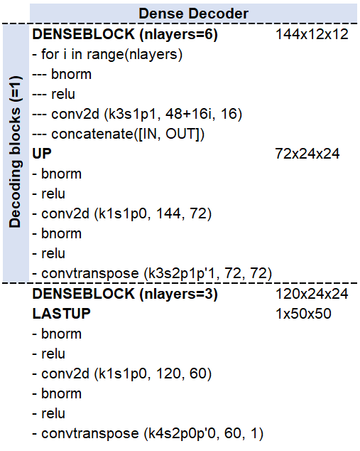
DenseNets [2016] choose convolutions that preserve identical dimensions between inputs and outputs, thereby permitting their concatenation. The input to any one layer is the last layer’s output concatenated with all previous inputs. This structure is particularly valuable when analyzing objects across multiple spatial scales. Each successive convolution reflects an expanding receptive field. A 1x1 convolution combines feature maps of varying receptive fields resulting in a network that readily adapts to local versus global phenomena. We present the structure of DenseED in Panel A of Figure 1 and detail the specific design of the encoder and decoder in Figures 2 and 3.
? (?) propose a strategy for modeling time-dependent outputs without altering the design of DenseED by broadcasting time across an input channel. We experiment with incorporating an LSTM [1997] to model transitions in the encoder-derived latent space henceforth referred to as DenseED-LSTM (Panel A of Figure 1). We hypothesize that an LSTM, with its memory and transition properties, is particularly apt to model a simulator’s dynamic behavior. The persistent cell state will house information about the permeability grid, which is relevant to prediction at every time step. Meanwhile, the hidden state-to-state transitions will receive a strong signal due to the autoregressive nature of the governing physics. Compared to DenseED, the encoder in DenseED-LSTM outputs twice as many feature maps (96 vs. 48). Half of those feature maps are used to initialize the first hidden state and half the first cell state. The LSTM outputs hidden state vectors for time steps which we decode to predict the saturation path.

Saturation Solutions and Alternative Treatment of Time-Dependence
| Train | Test | |
|---|---|---|
| DenseED | 0.991 | 0.840 |
| DenseED-LSTM | 0.941 | 0.847 |
We evaluate the performance of the surrogate in predicting the path of saturation with , where is a tensor describing the true saturation path for simulation and is the corresponding model prediction. The null model, from which we derive , predicts the mean image for all time steps. In Table 1, we record the test performance of DenseED and DenseED-LSTM which achieve similar degrees of success.
We further characterize the model’s performance by exploring how error varies in time and space. We expect time will influence error because the difficulty of the prediction task is non-uniform. Initially easy, prediction becomes difficult and then reverts to being easy again over short-, mid- and long-time horizons. The first images are easy to predict because water is initially only concentrated around the injector. As water floods the field, saturation enters a period of rapid flux. In this period, saturation at bears the least resemblance with its state at , and prediction is commensurately more difficult. Once saturation steadies, the model can issue a prediction at time at least as accurately as it did at . Therefore we expect performance to plateau at long time horizons. We observe that for both DenseED and DenseED-LSTM, follows this trend (Figure 4). Performance is highest when is near zero and deteriorates to a floor.

We also inspect individual test predictions to examine the spatial distribution of error. In Figure 5, we present one such prediction. We observe that for both DenseED and DenseED-LSTM error tends to be concentrated around the saturation front.

Once trained, the neural network can make very fast forward predictions. The CFD simulator took 10 seconds to finish each simulation when creating the synthetic dataset on an Intel Xeon 2.4GHz 128GB RAM Nvidia K80 workstation. For comparison, the neural network makes batch predictions on 1000 different permeability maps in less than a second on the same machine. The main time overhead of the neural network is in training. Still, it only takes 2 minutes to train DenseED for 200 epochs to predict a specific time instance with a Nvidia K80. In Figure 6, we show how test performance and training time vary with the number of simulations provided in training. Unsurprisingly the more simulations are provided in training, the better the model’s performance on the test set.

Global properties and Adversarial Effect
Unlike saturation which evolves at the speed of mass motion, pressure is a ”global” physics property established at the speed of sound, several orders of magnitude faster than the fluid’s convection speed. Therefore, the pressure solution is affected by the permeability of the entire region. In other words, the receptive field of pressure is global. Indeed, we find that we obtain the best validation results by adding one additional encoding and one additional upsampling block to the DenseED structure, which shrinks the bottleneck of the autoencoder from to . The smaller bottleneck further contains six -kernel convolutional layers, effectively resulting in a global receptive field of each pixel at the end of the bottleneck.
Fluid dynamic systems are known to have sharp spatial gradient and discontinuity like shocks. For example, the pressure solution scales as near the sources and sinks in 2D or cylindrical 3D space. This can lead to enormous spatial gradients close to the wells. Vanilla generative neural networks have difficulty in capturing such behavior because the regular distance-based losses lead to smoother, blurry results in an attempt to resemble many possible solutions. In the case of a fluid dynamic system, although the solution is unique for a given permeability map, we still found large-gradient results are more difficult to generate (see the 2nd row of Figure 7).

Generative Adversarial Networks (GAN) [2014] are well-known for creating sharp and visually realistic results by introducing a smart loss term learned by comparing the real and generated results. An additional discriminator is trained simultaneously to penalize the generator if it produces results that the discriminator easily discerns as fake. Similarly to ? (?), we adopt the final objective as
| (2) |
where is the DenseED autoencoder (generator), is the discriminator which has the same architecture as the encoder of DenseED plus a fully-connected layer to output binary prediction, and is the distance-based loss (L1-loss by default) between pixels of generated results and CFD results (true label). The adversarial loss term is given by
| (3) |
where is the permeability map input to DenseED, is the CFD result, and is the generated result. In ? (?), a conditional discriminator is utilized to judge if an image is real and also relevant to the input . In our case, although we do not find the conditional adversarial mechanism enhances the results notably, it does help stabilize the GAN training process. A fundamental difference between Eqn 3 and regular GAN is the absence of a randomly sampled latent vector. Once the permeability map is given, the fluid system’s dynamics are determined. Therefore, unlike a traditional GAN, we do not feed a random latent vector as input to the generator. The term in Eqn 2 is a weight quantifying the relative importance of GAN loss and is chosen to be so that the GAN loss is about 50% of L1 loss at the conclusion of the training cycle.
Figure 7 compares the pressure solutions from CFD, DenseED trained with L1 loss only and the same DenseED architecture trained with both L1 and GAN loss (Equation3). GAN loss helps significantly in capturing the large pressure gradient near the central injector. In comparison, L1-only DenseED produces consistently smoother results. Although the overall pixel-wise error of L1-only DenseED is smaller in many cases, the L1+GAN results are scientifically more accurate near the sink/source locations. This is critical because, in the real world, the sink/source locations are where the observable data are sampled.
Model Explanation and the Inverse Problem
Interpreting complex machine learning models such as deep neural networks is important because it helps humans understand the behavior of the model, vet whether the prediction is made based on the correct reasoning, and build even better models. Pixel-wise sensitivity and/or spatial attention maps have been used to help understand convolutional neural networks [2015, 2017, 2017, 2016]. Given that the deep learning models have been proven capable of accurately mimicking CFD numerical simulations, one important application is to explain the neural network model and uncover its underlying logic.
Considering saturation as a function of permeability and time , the ”pixel-wise” sensitivity of saturation to the permeability distribution can be quantified by
| (4) |
The partial in Equation4 represents how much saturation at location and time would change if the permeability at were a bit higher. In real cases, are the locations/time where the system is observed/measured. Given a fixed location of interest and a time , the local saturation sensitivity to permeability is a 2D slice of Eqn 4:
| (5) |
The sensitivity map helps us understand what consequences a slight alteration of the input physics laws may have on the system. However, the sensitivity map is extremely difficult to estimate using traditional CFD approaches because there is no explicit formula of . Instead, sensitivity must be calculated by forward computation at very high cost. In the given case, in order to numerically estimate on a 50x50 grid at time , simulations have to be run till this time step for each slightly perturbed input permeability map, which would take 7 hours on the same workstation. When the permeability distribution has to be updated iteratively, say, 100 times, in the inversion problem, the CFD-based approach would take more than one month.
Thanks to the deep-learning surrogate model, can be computed directly via backward propagation. Since DenseED and the convLSTM takes as input, the derivative of the output of the networks w.r.t. the ”pixels” of the input permeability map is the same as Eqn 5. We can also compute easily via numerical differentiation by running a batch of forward prediction at low cost. For the same example, evaluating six 2D at six different on the same workstation took only 619 ms, a 40,000-fold acceleration.
Figure 8 shows the saturation sensitivity map at six locations at time for a given permeability map from the test set. The particular chosen case is more permeable on the left half of the region, resulting in earlier water breakthrough in locations 1 and 3 than locations 2 and 4. As a result, the upper right and lower right corners have higher sensitivity to the permeability distribution between them and the central injector. The central point has zero sensitivity to the permeability map because it is always flooded immediately regardless. Location 6, which is located in a low permeability channel, is most sensitive to its upstream, the small region between itself and the central injector. In some sensitivity maps, certain regions have negative impact, indicating that an increase of permeability in those regions will actually result in a lower saturation; this is because those regions with a higher permeability will redirect some water to other directions and consequently give lower saturation at the locations of interest. The sensitivity maps, effectively obtained by locally linearizing the deep-learning-based surrogate model, honor the underlying physics very well, confirming the deep-learning model’s ability to capture the physics by learning from data.

The interpretation of the deep learning model lends itself to a powerful application. In the inverse problem, a dynamic system is governed by certain but not-yet-fully-determined laws. The goal is to find out the exact form of the governing laws so that the resulting dynamics satisfy all the observed data. In our case, the saturation at is observed and certain; however, the permeability distribution, which gives the exact form of the fluid dynamic equations, is not yet determined. The solution should be an optimal so that the resulting has minimized total discrepancy with all the observed data, i.e.,
| (6) |
where are the set of real measurements at locations/times . With L2 norm, the loss of the inverse problem is differentiable w.r.t. :
| (7) |
Given that can be readily evaluated with the deep-learning surrogate model, the above problem can be solved using gradient-based optimization methods iteratively via
where is the learning rate in the above gradient-descent iteration. In other words, in every iteration of the inversion optimization, the input permeability map is added/subtracted by a linear combination of the sensitivity maps shown in Figure 8, and then the sensitivity maps are recomputed to adjust for the change of the input permeability distribution. For instance, we perturbed the input permeability by adding times the sensitivity map 2 and subtracting times the sensitivity map 3, to obtain a desired saturation map (upper right corner of Figure 8) in which location 2 has higher saturation and location 4 has lower saturation.
We show in this section that model explanation offers an unprecedented advantage in solving the inverse problem, the true challenge that is not yet achievable with the traditional CFD method due to the limitation of computation power.
Summary and Discussion
We have presented a novel method of modeling a special fluid dynamic system with deep learning. We show that, by sampling a good distribution of exact form of the physics laws, it is possible to teach one unique deep learning model to capture the underlying physics and accurately simulate the dynamic system under each of the sampled physics law, and make prediction at high accuracy to new physics that were not explicitly provided in the training data; moreover, the deep learning approach provides a significantly faster way to forward evaluate the system, potentially helping solve the motivating inverse problem. The nonlinear partial dependence of the system behavior to the imposed physics can be quantified using the techniques of neural network explanation. This provides a much easier way to solve the inverse problem that would otherwise be infeasible using traditional numerical methods due to their high cost.
References
- [2015] Bach, S.; Binder, A.; Montavon, G.; Klauschen, F.; Müller, K.-R.; and Samek, W. 2015. On pixel-wise explanations for non-linear classifier decisions by layer-wise relevance propagation. PLoS ONE 10(7):1–46.
- [2015] Badrinarayanan, V.; Kendall, A.; and Cipolla, R. 2015. SegNet: A Deep Convolutional Encoder-Decoder Architecture for Image Segmentation. arXiv:1511.00561 [cs]. arXiv: 1511.00561.
- [1928] Courant, R.; Friedrichs, K.; and Lewy, H. 1928. Über die partiellen differenzengleichungen der mathematischen physik. Mathematische Annalen 100(1):32–74.
- [2009] Deng, J.; Dong, W.; Socher, R.; Li, L.-J.; Li, K.; and Fei-Fei, L. 2009. ImageNet: A Large-Scale Hierarchical Image Database. In CVPR09.
- [2017] Farimani, A. B.; Gomes, J.; and Pande, V. S. 2017. Deep Learning the Physics of Transport Phenomena. arXiv:1709.02432 [physics]. arXiv: 1709.02432.
- [2014] Goodfellow, I.; Pouget-Abadie, J.; Mirza, M.; Xu, B.; Warde-Farley, D.; Ozair, S.; Courville, A.; and Bengio, Y. 2014. Generative adversarial nets. In Ghahramani, Z.; Welling, M.; Cortes, C.; Lawrence, N. D.; and Weinberger, K. Q., eds., Advances in Neural Information Processing Systems 27. Curran Associates, Inc. 2672–2680.
- [2016] Guo, X.; Li, W.; and Iorio, F. 2016. Convolutional Neural Networks for Steady Flow Approximation. In Proceedings of the 22Nd ACM SIGKDD International Conference on Knowledge Discovery and Data Mining, KDD ’16, 481–490. New York, NY, USA: ACM. event-place: San Francisco, California, USA.
- [2015] He, K.; Zhang, X.; Ren, S.; and Sun, J. 2015. Deep residual learning for image recognition. CoRR abs/1512.03385.
- [1997] Hochreiter, S., and Schmidhuber, J. 1997. Long Short-Term Memory. Neural Comput. 9(8):1735–1780.
- [2016] Huang, G.; Liu, Z.; van der Maaten, L.; and Weinberger, K. Q. 2016. Densely Connected Convolutional Networks. arXiv:1608.06993 [cs]. arXiv: 1608.06993.
- [2016] Isola, P.; Zhu, J.-Y.; Zhou, T.; and Efros, A. A. 2016. Image-to-Image Translation with Conditional Adversarial Networks. arXiv:1611.07004 [cs]. arXiv: 1611.07004.
- [2015] Ladický, L.; Jeong, S.; Solenthaler, B.; Pollefeys, M.; and Gross, M. 2015. Data-driven Fluid Simulations Using Regression Forests. ACM Trans. Graph. 34(6):199:1–199:9.
- [2014] Long, J.; Shelhamer, E.; and Darrell, T. 2014. Fully Convolutional Networks for Semantic Segmentation. 10.
- [2017] Lundberg, S. M., and Lee, S.-I. 2017. A unified approach to interpreting model predictions. In Guyon, I.; Luxburg, U. V.; Bengio, S.; Wallach, H.; Fergus, R.; Vishwanathan, S.; and Garnett, R., eds., Advances in Neural Information Processing Systems 30. Curran Associates, Inc. 4765–4774.
- [2019a] Mo, S.; Zabaras, N.; Shi, X.; and Wu, J. 2019a. Integration of adversarial autoencoders with residual dense convolutional networks for inversion of solute transport in non-Gaussian conductivity fields. arXiv:1906.11828 [physics, stat]. arXiv: 1906.11828.
- [2019b] Mo, S.; Zhu, Y.; Zabaras, N.; Shi, X.; and Wu, J. 2019b. Deep convolutional encoder-decoder networks for uncertainty quantification of dynamic multiphase flow in heterogeneous media. Water Resources Research 55(1):703–728. arXiv: 1807.00882.
- [2018] Paganini, M.; de Oliveira, L.; and Nachman, B. 2018. Accelerating Science with Generative Adversarial Networks: An Application to 3d Particle Showers in Multi-Layer Calorimeters. Physical Review Letters 120(4):042003. arXiv: 1705.02355.
- [2017a] Raissi, M.; Perdikaris, P.; and Karniadakis, G. E. 2017a. Physics Informed Deep Learning (Part I): Data-driven Solutions of Nonlinear Partial Differential Equations. arXiv:1711.10561 [cs, math, stat]. arXiv: 1711.10561.
- [2017b] Raissi, M.; Perdikaris, P.; and Karniadakis, G. E. 2017b. Physics Informed Deep Learning (Part II): Data-driven Discovery of Nonlinear Partial Differential Equations. arXiv:1711.10566 [cs, math, stat]. arXiv: 1711.10566.
- [] Shi, X.; Chen, Z.; Wang, H.; Yeung, D.-Y.; Wong, W.-k.; and Woo, W.-c. Convolutional LSTM Network: A Machine Learning Approach for Precipitation Nowcasting. 9.
- [2017] Smilkov, D.; Thorat, N.; Kim, B.; Viégas, F. B.; and Wattenberg, M. 2017. Smoothgrad: removing noise by adding noise. CoRR abs/1706.03825.
- [2016] Tompson, J.; Schlachter, K.; Sprechmann, P.; and Perlin, K. 2016. Accelerating Eulerian Fluid Simulation With Convolutional Networks. arXiv:1607.03597 [cs]. arXiv: 1607.03597.
- [] Wang, Y.; Long, M.; Wang, J.; Gao, Z.; and Yu, P. S. PredRNN: Recurrent Neural Networks for Predictive Learning using Spatiotemporal LSTMs. 10.
- [2018] Wiewel, S.; Becher, M.; and Thuerey, N. 2018. Latent-space Physics: Towards Learning the Temporal Evolution of Fluid Flow. arXiv:1802.10123 [cs]. arXiv: 1802.10123.
- [2016] Zagoruyko, S., and Komodakis, N. 2016. Paying more attention to attention: Improving the performance of convolutional neural networks via attention transfer. CoRR abs/1612.03928.
- [2018] Zhu, Y., and Zabaras, N. 2018. Bayesian Deep Convolutional Encoder-Decoder Networks for Surrogate Modeling and Uncertainty Quantification. Journal of Computational Physics 366:415–447. arXiv: 1801.06879.
- [2017] Zhu, J.; Park, T.; Isola, P.; and Efros, A. A. 2017. Unpaired image-to-image translation using cycle-consistent adversarial networks. CoRR abs/1703.10593.
- [2019] Zhu, Y.; Zabaras, N.; Koutsourelakis, P.-S.; and Perdikaris, P. 2019. Physics-Constrained Deep Learning for High-dimensional Surrogate Modeling and Uncertainty Quantification without Labeled Data. Journal of Computational Physics 394:56–81. arXiv: 1901.06314.
*