跳到论文正文
W Papers独立论文阅读器 arXiv:2006.05147 论文正文 计算阅读时间 · 0%
引用这篇论文根据当前论文元数据生成,正式投稿前建议核对。


License: CC BY 4.0
arXiv:2006.05147v4 [eess.SP] 12 Sep 2021

Multiuser Full-Duplex Two-Way Communications via Intelligent Reflecting Surface

Zhangjie Peng    Zhenkun Zhang    Cunhua Pan    Li Li    and A. Lee Swindlehurst    Thanks: Z. Peng is with the College of Information, Mechanical and Electrical Engineering, Shanghai Normal University, Shanghai 200234, China, and also with the National Mobile Communications Research Laboratory, Southeast University, Nanjing 210096, China (e-mail: pengzhangjie@shnu.edu.cn). L. Li and Z. Zhang are with the College of Information, Mechanical and Electrical Engineering, Shanghai Normal University, Shanghai 200234, China (e-mails: lilyxuan@shnu.edu.cn, 1000479070@smail.shnu.edu.cn). C. Pan is with the School of Electronic Engineering and Computer Science at Queen Mary University of London, London E1 4NS, U.K. (e-mail: c.pan@qmul.ac.uk). A. L. Swindlehurst is with the Department of Electrical Engineering and Computer Science, University of California at Irvine, Irvine, CA 92697 USA (e-mail: swindle@uci.edu). The work of Z. Peng was supported in part by the NSFC under 61701307, and the open research fund of National Mobile Communications Research Laboratory, Southeast University (No. 2018D14); the work of A. L. Swindlehurst was supported in part by the U.S. National Science Foundation under grant ECCS-2030029. (Corresponding author: Cunhua Pan and Zhenkun Zhang)
Abstract

Low-cost passive intelligent reflecting surfaces (IRSs) have recently been envisioned as a revolutionary technology capable of reconfiguring the wireless propagation environment through carefully tuning reflection elements. This paper proposes deploying an IRS to cover the dead zone of cellular multiuser full-duplex (FD) two-way communication links while suppressing user-side self-interference (SI) and co-channel interference (CI). This approach, allowing the base station (BS) and all users to exchange information simultaneously, can potentially double the spectral efficiency. To ensure network fairness, we jointly optimize the precoding matrix of the BS and the reflection coefficients of the IRS to maximize the weighted minimum rate (WMR) of all users, subject to maximum transmit power and unit-modulus constraints. We reformulate this non-convex problem and decouple it into two subproblems. Then the optimization variables in the equivalent problem are alternately optimized by adopting the block coordinate descent (BCD) algorithm. In order to further reduce the computational complexity, we propose the minorization-maximization (MM) algorithm for optimizing the precoding matrix and the reflection coefficient vector by defining minorizing functions in the surrogate problems. Finally, simulation results confirm the convergence and efficiency of our proposed algorithm, and validate the advantages of introducing IRS to improve coverage in blind areas.

Index Terms: 
Intelligent Reflecting Surface (IRS), Reconfigurable Intelligent Surface (RIS), max-min fairness (MMF), Full-Duplex, Two-way Communications.

I Introduction

In the future 5G-and-beyond era, wireless networks will be required to achieve a 1000-fold increase in capacity compared with current networks, motivated by the growing popularity of applications that rely on high data rate transmission, such as three-dimensional (3D) video and augmented reality (AR) [1]. To achieve this progress, promising techniques such as millimeter wave (mmWave) communication, ultra-dense cloud radio access networks (UD-CRAN) [2] and massive multiple-input multiple-output (M-MIMO) arrays [3] have been advocated [4]. In addition, full-duplex (FD) two-way communication in which two or more devices simultaneously exchange data at the same carrier frequency has received extensive research attention as it can double the spectral-efficiency of the wireless communication system [5, 6]. Due to its appealing advantages, two-way FD relaying has been extensively studied in various scenarios, such as D2D communications [5], cognitive radio [7], mmWave communication [8] and M-MIMO [9]. However, an FD two-way network suffers from low energy-efficiency and high hardware cost. For example, the large number of antennas in M-MIMO leads to a large number of RF chains and incurs high power consumption, while energy-intensive transceivers and complex signal processing techniques are required to support the mmWave communication. Moreover, another non-negligible bottleneck in the implementation of FD two-way communications lies in the propagation environment. In particular, besides the loop-interference (LI) at the relay, this network must also overcome back-propagation interference at the base station (BS) and the users.

Thanks to breakthroughs in micro-electrical-mechanical systems and programmable metamaterials, the intelligent reflecting surfaces (IRSs) have recently attracted extensive attention from researchers as a means to improve both the spectral- and energy-efficiency of wireless communications networks [10], and to enable the future vision of smart radio environments [11]. An IRS comprises a number of low-cost passive reflection elements requiring no dedicated energy sources [12], and each reflection element can independently impose a continuously or discretely tunable phase shift onto the incident signal [13, 14]. When the phase shifts are properly adjusted, the directly transmitted signal and the reflected signal can be superimposed constructively at the intended receivers or destructively at other unintended users. Note that an IRS can also implement fine-grained 3D passive beamforming [15], and thus its function resembles that of an FD MIMO amplify-and-forward (AF) relay. The difference is that the IRS transmits signals through passive reflection, requiring no signal processing to deal with LI and leading to negligible energy consumption. In addition, unlike active relay transmission, an IRS does not generate new signals or thermal noise. Thanks to its miniaturized circuits, an IRS also has the attractive advantages of light weight, small size and high integration, which enables it to be used to improve indoor propagation environments [16]. For outdoor communication scenarios, it can be integrated into the existing infrastructure, such as building facades, station signs and lampposts.

Due to these promising features, joint precoding at the BS/AP and reflecting at the IRS has been extensively studied in one-way communication networks, for the MISO case [17, 18, 19, 20], physical layer security [18, 21, 22], simultaneous wireless information and power transfer (SWIPT) [23], mobile edge computing [24], and multigroup multicast [25]. In addition, the deep reinforcement learning technique has been leveraged for this joint design [26]. More system factors, such as channel estimation and the overhead required for configuring the phase shifts, are taken into account in recent works [27]. However, there is a paucity of investigations on the study of the integration of IRS in two-way communications [28, 29, 30]. The work of [28] and [29] considered communication between two SISO end users and two MIMO sources, respectively, both of which are aimed at maximizing the system sum rate. A cognitive radio system consisting of an FD BS and multiple half-duplex users was considered in [30], where the system sum rate of the secondary network was maximized with a constraint on the interference to the primary users. However, the fairness between uplink and downlink transmissions needs to be guaranteed in FD communication, and this has not been taken into account in these studies.

In this paper, we propose to employ an IRS in an FD two-way network to provide signal coverage for users in blind areas, as shown in Fig. 1. Specifically, unlike the relay schemes in [31], in our proposed system, both the uplink and downlink transmissions can occur simultaneously and operate at the same frequency via the reflection of the IRS, and thus potentially doubles the spectral-efficiency. In order to guarantee fairness, the max-min fairness (MMF) criterion is chosen as the optimization metric, which is a complex non-differentiable objective function (OF) that cannot be solved by applying the existing methods proposed in the related works such as [17].

Refer to caption
Fig. 1: Illustration of the IRS-aided FD two-way communication between a MIMO BS and KK SISO users.

We summarize the main contributions and challenges of this work as follows

  1. 1.

    To the best of our knowledge, this is the first work to consider fairness in a multiuser FD two-way communication network with the assistance of an IRS. Specifically, we jointly optimize the precoding matrix of the BS and the reflection coefficients of the IRS to maximize the weighted minimum rate (WMR) of all users, subject to maximum transmit power and unit modulus constraints. This problem is challenging to tackle for the non-differentiable OF and the highly coupled optimization variables.

  2. 2.

    By applying the weighted minimum mean-square error (WMMSE) criterion and introducing certain auxiliary variables, the original problem is transformed and solved effectively through the proposed block coordinate descent (BCD) algorithm, in which each set of variables is alternately optimized. In particular, the precoding subproblem is formulated as a second-order cone programming problem (SOCP), and the reflection coefficient subproblem is derived as a quasi-SOCP with a non-convex quadratic constraint.

  3. 3.

    In order to further reduce the computational complexity of the BCD algorithm, we proposed a modified Minorization-Maximization (MM) algorithm. Specifically, unlike the quadratic form in [20], the OFs of both subproblems are non-differentiable. We thus utilize the smooth approximation theory [32] to obtain differentiable approximations for them. Then, the corresponding minorizing functions are derived sequentially, which leads to surrogate problems with closed-form solutions. Hence, both approximated subproblems are solved efficiently by the MM algorithm in an iterative manner.

  4. 4.

    Our simulation results illustrate the feasibility of the proposed approach and the advantages of using an IRS in assisting the FD two-way communication. Additionally, the results also provide guidance for practical engineering designs, and highlight the trade-off between improved self-interference (SI) elimination when the IRS is deployed near the users, and reduced propagation blockages when the IRS is deployed near the BS. The convergence and the efficiency of the proposed algorithm are also verified.

The rest of the paper is organized as follows. Section II describes the system model involving multiuser FD two-way communication via an IRS, and formulates the WMR maximization problem. In Section III, we derive the subproblems corresponding to each set of variables by reformulating the original problem and performing alternating optimization. In Section IV, we propose a low-complexity version of the algorithm. Extensive simulation results are presented in Section V. Finally, we conclude the paper in Section VI.

Notation: Vectors and matrices are denoted by boldface lower and boldface capital case letters, respectively. The quantities 𝐚m{\bf a}_{m} and 𝐀m,n{\bf A}_{m,n} respectively denote the mmth element of vector 𝐚\bf a and the (m,n)\left(m,n\right)-entry of matrix 𝐀\bf A. ℂM×N{{\mathbb{C}}^{{M}\times N}} denotes the space of M×N{{M}\times N} complex-valued matrices, and j≜−1j\triangleq\sqrt{{\rm{-1}}} is the imaginary unit. 𝐀H{\bf A}^{\rm H}, 𝐀T{\bf A}^{\rm T} and 𝐀∗{\bf A}^{*} denote the Hermitian, transpose and conjugate of matrix 𝐀{\bf A}, respectively. The trace and Frobenius norm of a matrix are denoted by Tr⁡[⋅]{\rm Tr}\left[\cdot\right] and ‖⋅‖F\left\|\cdot\right\|_{F}, respectively. ‖⋅‖1\left\|\cdot\right\|_{1} and ‖⋅‖2\left\|\cdot\right\|_{2} denote the l1l_{1}- and l2l_{2}-norm of a vector, respectively. For a complex scalar aa, Re​{a}{\rm Re}\left\{a\right\}, 𝔼⁡[a]{\mathbb{E}}\left[a\right], |a|\left|a\right| and ∠⁡(a)\angle\left(a\right) denote the real part, expectation, absolute value and angle of aa, respectively. The functions diag⁡(⋅){\rm diag}\left(\cdot\right) and vec⁡(⋅){\rm vec}\left(\cdot\right) represent diagonalization and vectorization operators. 𝐀⪰𝐁{\bf A}\succeq{\bf B} means that 𝐀−𝐁{\bf A}-{\bf B} is a positive semidefinite matrix. The Hadamard product and Kronecker product of 𝐀{\bf A} and 𝐁{\bf B} are respectively denoted by 𝐀⊙𝐁{\bf A}\odot{\bf B} and 𝐀⊗𝐁{\bf A}\otimes{\bf B}. 𝒞​𝒩​(0,σ2){\mathcal{C}}{\mathcal{N}}(0,\sigma^{2}) denotes the Gaussian distribution with mean 00 and variance σ2\sigma^{2}.

II System Model and Problem Formulation

II-A Signal Transmission Model

Consider an FD two-way communication system with one BS and multiple users, where both the downlink and uplink transmissions occur at the same time and the same frequency as shown in Fig. 1. Due to path loss and blockages, no direct link between the BS and the users is assumed to exist. An IRS is deployed to assist the data transmission by establishing additional non-line-of-sight (NLoS) links.

The BS is equipped with Nt>1{N_{\rm{t}}}>1 transmit antennas and Nr>1{N_{\rm{r}}}>1 receive antennas. In the service area of the IRS, there are KK users, each equipped with a pair of transmit and receive antennas. Additionally, we assume that each user transmits signals with a fixed power.

The signal transmitted from the BS is given by

𝐱D=∑k=1K𝐟k​sD,k,{\bf{x}}_{\rm{D}}=\sum\limits_{k=1}^{K}{{{\bf{f}}_{k}}{s_{{\rm{D}},k}}}, (1)

where sD,k{{s_{{\rm{D}},k}}} denotes the desired data symbol for user kk and 𝐟k∈ℂNt×1{{\mathbf{f}}_{k}}\in{{\mathbb{C}}^{{N_{\rm t}}\times 1}} is the corresponding beamforming vector. Similarly, the transmit signal at user kk is

xU,k=Pk​sU,k,{x_{{\rm{U}},k}}=\sqrt{{P_{k}}}{s_{{\rm{U}},k}}, (2)

where sU,ks_{{\rm{U}},k} denotes the data symbol sent by user kk, and PkP_{k} is the corresponding transmit power. Defining ℒ={D,U}{\mathcal{L}}=\left\{{{\rm{D}},{\rm{U}}}\right\} and 𝒦={1,⋯,K}{\mathcal{K}}=\left\{{1,\cdots,K}\right\}, we assume each sl,ks_{l,k} for ∀l∈ℒ,k∈𝒦\forall l\in{\mathcal{L}},k\in{\mathcal{K}} is an independent Gaussian data symbol and has unit power, i.e., 𝔼⁡[sl,k​sl,k∗]=1{\mathbb{E}}\left[{{s_{l,k}}s_{l,k}^{\ast}}\right]=1 and 𝔼⁡[sl,k​si,j∗]=0{\mathbb{E}}\left[{{s_{l,k}}s_{i,j}^{\ast}}\right]=0, {l,k}≠{i,j}\left\{{l,k}\right\}\neq\left\{{i,j}\right\}. Let us denote 𝐅=[𝐟1,⋯,𝐟K]∈ℂNt×K{\mathbf{F}}=\left[{{{\mathbf{f}}_{1}},\cdots,{{\mathbf{f}}_{K}}}\right]\in{{\mathbb{C}}^{{N_{t}}\times K}} as the collection of all beamforming vectors, so that the power constraint of the BS can be written as

𝒮F={𝐅|Tr[𝐅H​𝐅]≤Pmax},{{\mathcal{S}}_{F}}=\left\{{{\mathbf{F}}|{\mathop{\rm Tr}}\left[{{{\mathbf{F}}^{\rm H}}{\mathbf{F}}}\right]\leq{P_{\rm max}}}\right\}, (3)

where Pmax{P_{\rm{max}}} is the maximum transmit power of the BS.

The IRS contains MM passive reflection elements that adjust the phases of incident signals. The set of reflection coefficients is represented as the vector ϕ=[ϕ1,⋯,ϕM]T\bm{\phi}={\left[{{\phi_{1}},\cdots,{\phi_{M}}}\right]^{\rm T}}, or equivalently as a matrix of 𝚽=d​i​a​g​(ϕ){\bm{\Phi}}=diag\left(\bm{\phi}\right), where |ϕm|2=1{\left|\phi_{m}\right|^{2}}=1, ∀m=1,⋯,M\forall m=1,\cdots,M. In order to provide efficient transmission, the antenna spacing at the BS should be large enough so that the small-scale fading associated with two different antennas can be assumed independent. A similar assumption holds for the reflection elements of the IRS. The baseband channels from the BS to the IRS, from the IRS to the BS, from user kk to the IRS, and from the IRS to user kk are denoted by 𝐆t∈ℂM×Nt{\mathbf{G}_{\rm t}}\in{{\mathbb{C}}^{M\times{N_{\rm t}}}}, 𝐆r∈ℂM×Nr{\mathbf{G}_{\rm r}}\in{{\mathbb{C}}^{M\times{N_{\rm r}}}}, 𝐡t,k∈ℂM×1{\mathbf{h}_{{\rm t},k}}\in{{\mathbb{C}}^{M\times 1}}, and 𝐡r,k∈ℂM×1{\mathbf{h}_{{\rm r},k}}\in{{\mathbb{C}}^{M\times 1}}, respectively. Furthermore, we denote the loop channels between the transmit and receive antenna(s) of user kk and the BS by hk​kh_{kk} and 𝐇B{{{\bf{H}}_{\rm B}}}, respectively. The CSI for all channels is assumed to be quasi-static and perfectly known by the BS. 11 1 Though this assumption is idealistic, it allows us to explore the upper bounds for the performance of IRS-based FD networks. The robust transmission design based on imperfect CSI was studied in [33] for a multiuser half-duplex system, and its extension to FD systems will be left for future work.

The signal received by user kk can be modeled as

yD,k\displaystyle{y_{{\rm{D}},k}} =𝐡r,kH​𝚽​𝐆t​𝐟k​sD,k+∑m=1m≠kK𝐡r,kH​𝚽​𝐆t​𝐟m​sD,m⏟Multiuser interference\displaystyle={\bf{h}}_{{\rm r},k}^{\rm{H}}{\bf{\Phi}}{{\bf{G}}_{\rm t}}{{\bf{f}}_{k}}{s_{{\rm{D}},k}}+\underbrace{\sum\limits_{\begin{subarray}{c}m=1\\ m\neq k\end{subarray}}^{K}{{\bf{h}}_{{\rm r},k}^{\rm{H}}{\bf{\Phi}}{{\bf{G}}_{\rm t}}{{\bf{f}}_{m}}{s_{{\rm{D}},m}}}}_{{\text{Multiuser interference}}}
+ρL​Pk​hk​k​sU,k⏟Loop-interference+ρS​Pk​𝐡r,kH​𝚽​𝐡t,k​sU,k⏟Self-interference\displaystyle\quad+\underbrace{\sqrt{{\rho_{\rm{L}}}}\sqrt{{P_{k}}}{h_{kk}}{s_{{\rm{U}},k}}}_{{\text{Loop-interference}}}+\underbrace{\sqrt{{\rho_{\rm{S}}}}\sqrt{{P_{k}}}{\bf{h}}_{{\rm r},k}^{\rm{H}}{\bf{\Phi}}{{\bf{h}}_{{\rm t},k}}{s_{{\rm{U}},k}}}_{{\text{Self-interference}}}
+∑m=1m≠kKPm​𝐡r,kH​𝚽​𝐡t,m​sU,m⏟Co-channel interference+nk,\displaystyle\quad+\underbrace{\sum\limits_{\begin{subarray}{c}m=1\\ m\neq k\end{subarray}}^{K}{\sqrt{{P_{m}}}{\bf{h}}_{{\rm r},k}^{\rm{H}}{\bf{\Phi}}{{\bf{h}}_{{\rm t},m}}{s_{{\rm{U}},m}}}}_{{\text{Co-channel interference}}}+{n_{k}}, (4)

where ρL{\rho}_{\rm L} and ρS{\rho_{\rm S}} with 0≤ρL,ρS≤10\leq{\rho_{\rm L}},{\rho_{\rm S}}\leq 1 are LI and SI coefficients, respectively, and nkn_{k} is additive white Gaussian noise (AWGN) following the distribution 𝒞​𝒩​(0,σk2){\mathcal{C}}{\mathcal{N}}(0,\sigma_{k}^{2}). The coefficient ρL\rho_{\rm L} is introduced to model the fact that LI suppression methods such as antenna isolation may not completely eliminate the LI. Similarly, SI elimination methods can to some extent reduce the influence of SI reflected from the IRS, 22 2 According to (II-A), to partially eliminate the SI, the scalar 𝐡r,kH​𝚽​𝐡t,k{\bf{h}}_{{\rm r},k}^{\rm{H}}{\bf{\Phi}}{{\bf{h}}_{{\rm t},k}} should be estimated by each user, for example as follows. After the reflection coefficients of the IRS calculated at the BS are sent to the IRS controller, the BS remains silent and the IRS works with the calculated reflection coefficients. Then, each user sends one or more pilot symbols to estimate the scalar channel 𝐡r,kH​𝚽​𝐡t,k{\bf{h}}_{{\rm r},k}^{\rm{H}}{\bf{\Phi}}{{\bf{h}}_{{\rm t},k}} while the other users remain silent. This step is repeated until all users have estimated their channels. and thus we also introduce the coefficient ρS\rho_{\rm S} to model the residual SI component. Due to blockages as shown in Fig. 1, the user-to-user interference contribution will likely be small, and thus we treat it as AWGN and include it in nkn_{k}. In particular, we denote the sum of the LI term and nkn_{k} in (II-A) as iD,ki_{{\rm{D}},k}, whose average power is given by σD,k2=|iD,k|2=ρL​Pk​|hk​k|2+σk2\sigma_{{\rm{D}},k}^{2}={\left|{{i_{{\rm{D}},k}}}\right|^{2}}={{\rho}_{\rm{L}}}{P_{k}}{\left|{{h_{kk}}}\right|^{2}}+\sigma_{k}^{2}. Then, the signal-to-interference-plus-noise ratio (SINR) at user kk is given by

γD,k=|𝐡r,kH​𝚽​𝐆t​𝐟k|2∑m=1m≠kK|𝐡r,kH​𝚽​𝐆t​𝐟m|2+∑m=1Kρ​Pm​|𝐡r,kH​𝚽​𝐡t,m|2+σD,k2,{\gamma_{{\rm{D}},k}}=\frac{{{{\left|{{\bf{h}}_{{\rm r},k}^{\rm H}{\bf{\Phi}}{{\bf{G}}_{\rm t}}{{\bf{f}}_{k}}}\right|}^{2}}}}{{\sum\limits_{\begin{subarray}{c}m=1\\ m\neq k\end{subarray}}^{K}{{{\left|{{\bf{h}}_{{\rm r},k}^{\rm H}{\bf{\Phi}}{{\bf{G}}_{\rm t}}{{\bf{f}}_{m}}}\right|}^{2}}}+\sum\limits_{m=1}^{K}{{\rho}}{{P_{m}}{{\left|{{\bf{h}}_{{\rm r},k}^{\rm H}{\bf{\Phi}}{{\bf{h}}_{{\rm t},m}}}\right|}^{2}}}+\sigma_{{\rm{D}},k}^{2}}}, (5)

where the coefficient ρ{\rho} is defined as

ρ={ρS,if​m=k;1,otherwise.{\rho}=\begin{cases}{\rho_{\rm{S}}},&\text{if}\ m=k;\\ 1,&\text{otherwise}.\end{cases}


eU,k\displaystyle{e_{{\rm{U}},k}} =𝔼⁡[(s^U,k−sU,k)H​(s^U,k−s^U,k)]\displaystyle=\mathbb{E}\left[{{{\left({{{\hat{s}}_{{\rm{U}},k}}-{s_{{\rm{U}},k}}}\right)}^{\rm{H}}}\left({{{\hat{s}}_{{\rm{U}},k}}-{{\hat{s}}_{{\rm{U}},k}}}\right)}\right]
=(Pk​𝐮U,kH​𝐆rH​𝚽​𝐡t,k−1)H​(Pk​𝐮U,kH​𝐆rH​𝚽​𝐡t,k−1)+∑m=1,m≠kKPm​𝐮U,kH​𝐆rH​𝚽​𝐡t,m​𝐡t.mH​𝚽H​𝐆r​𝐮U,k+σU2​Nr​𝐮U,kH​𝐮U,k\displaystyle=\left({\sqrt{{P_{k}}}{\bf{u}}_{{\rm{U}},k}^{\rm H}{\bf{G}}_{\rm r}^{\rm H}{\bf{\Phi}}{{\bf{h}}_{{\rm t},k}}-1}\right)^{\rm H}{\left({\sqrt{{P_{k}}}{\bf{u}}_{{\rm{U}},k}^{\rm H}{\bf{G}}_{\rm r}^{\rm H}{\bf{\Phi}}{{\bf{h}}_{{\rm t},k}}-1}\right)}+\sum\limits_{m=1,m\neq k}^{K}{{P_{m}}{\bf{u}}_{{\rm{U}},k}^{\rm H}{\bf{G}}_{\rm r}^{\rm H}{\bf{\Phi}}{{\bf{h}}_{{\rm t},m}}{\bf{h}}_{{\rm t}.m}^{\rm H}{{\bf{\Phi}}^{\rm H}}{{\bf{G}}_{\rm r}}{{\bf{u}}_{{\rm{U}},k}}}+\sigma_{\rm{U}}^{2}{N_{\rm r}}{\bf{u}}_{{\rm{U}},k}^{\rm H}{{\bf{u}}_{{\rm{U}},k}}
=∑m=1KPm​𝐮U,kH​𝐆rH​𝚽​𝐡t,m​𝐡t.mH​𝚽H​𝐆r​𝐮U,k−2​Re{Pk​𝐮U,kH​𝐆rH​𝚽​𝐡t,k}+σU2​𝐮U,kH​𝐮U,k+1.\displaystyle=\sum\limits_{m=1}^{K}{{P_{m}}{\bf{u}}_{{\rm{U}},k}^{\rm H}{\bf{G}}_{\rm r}^{\rm H}{\bf{\Phi}}{{\bf{h}}_{{\rm t},m}}{\bf{h}}_{{\rm t}.m}^{\rm H}{{\bf{\Phi}}^{\rm H}}{{\bf{G}}_{\rm r}}{{\bf{u}}_{{\rm{U}},k}}}-2{\mathop{\rm Re}\nolimits}\left\{{\sqrt{{P_{k}}}{\bf{u}}_{{\rm{U}},k}^{\rm H}{\bf{G}}_{\rm r}^{\rm H}{\bf{\Phi}}{{\bf{h}}_{{\rm t},k}}}\right\}+\sigma_{\rm{U}}^{2}{\bf{u}}_{{\rm{U}},k}^{\rm H}{{\bf{u}}_{{\rm{U}},k}}+1. (13)

Similarly, the signal received at the BS 𝐲U∈ℂNr×1{{\mathbf{y}}_{\rm U}}\in{{\mathbb{C}}^{{N_{r}}\times 1}} is given by

𝐲U\displaystyle{{\bf{y}}_{\rm{U}}} =𝐆rH​𝚽​𝐡t,k​Pk​sU,k+∑m=1m≠kK𝐆rH​𝚽​𝐡t,m​Pm​sU,m⏟Multiuser interference\displaystyle={\bf{G}}_{\rm r}^{\rm H}{\bf{\Phi}}{{\bf{h}}_{{\rm t},k}}\sqrt{{P_{k}}}{s_{{\rm{U}},k}}+\underbrace{\sum\limits_{\begin{subarray}{c}m=1\\ m\neq k\end{subarray}}^{K}{{\bf{G}}_{\rm r}^{\rm H}{\bf{\Phi}}{{\bf{h}}_{{\rm t},m}}\sqrt{{P_{m}}}{s_{{\rm{U}},m}}}}_{{\text{Multiuser interference}}}
+𝐇B​∑m=1K𝐟m​sD,m⏟Loop-interference+𝐆rH​𝚽​𝐆t​∑m=1K𝐟m​sD,m⏟Self-interference+𝐧B,\displaystyle\quad+\underbrace{{{\bf{H}}_{\rm{B}}}\sum\limits_{m=1}^{K}{{{\bf{f}}_{m}}}{s_{{\rm{D}},m}}}_{{\text{Loop-interference}}}+\underbrace{{\bf{G}}_{\rm r}^{\rm H}{\bf{\Phi}}{{\bf{G}}_{\rm t}}\sum\limits_{m=1}^{K}{{{\bf{f}}_{m}}}{s_{{\rm{D}},m}}}_{{\text{Self-interference}}}+{{\bf{n}}_{\rm{B}}}, (6)

where 𝐧B{\bf{n}}_{\rm{B}} is the AWGN noise vector, whose elements are independently distributed as 𝒞𝒩⁡(0,σB2){\cal C}{\cal N}(0,\sigma_{\rm{B}}^{2}). Based on techniques for LI cancellation for FD AF MIMO relays [34, 35], we assume the BS LI can be effectively eliminated. With the calculated reflection coefficients of the IRS, the SI received at the BS is known and can be effectively mitigated. We assume that any residual noise resulting from the interference cancellation is i.i.d. AWGN, denote σU2\sigma_{\rm{U}}^{2} as the average power of the total noise at the BS, and define in∼𝒞𝒩⁡(0,σU2){i_{n}}\sim{\cal C}{\cal N}(0,\sigma_{\rm{U}}^{2}), n=1,…,Nrn=1,\dots,N_{\rm r}. Then (II-A) can be simplified to

𝐲U=𝐆rH​𝚽​𝐡t,k​Pk​sU,k+∑m=1m≠kK𝐆rH​𝚽​𝐡t,m​Pm​sU,m+𝐢B,\displaystyle{{\bf{y}}_{\rm{U}}}={\bf{G}}_{\rm r}^{\rm{H}}{\bf{\Phi}}{{\bf{h}}_{{\rm t},k}}\sqrt{{P_{k}}}{s_{{\rm{U}},k}}+\sum\limits_{\begin{subarray}{c}m=1\\ m\neq k\end{subarray}}^{K}{{\bf{G}}_{\rm r}^{\rm{H}}{\bf{\Phi}}{{\bf{h}}_{{\rm t},m}}\sqrt{{P_{m}}}{s_{{\rm{U}},m}}}+{{\bf{i}}_{\rm{B}}}, (7)

where 𝐢B≜[i1,…,iNr]T{{\bf{i}}_{\rm{B}}}\triangleq\left[{i_{1},\dots,i_{N_{\rm r}}}\right]^{\rm T}.

Denoting the set of receive beamformers at the BS by 𝒰U={𝐮U,k,∀k∈𝒦}{{\mathcal{U}}_{\rm{U}}}={\left\{{{{\bf{u}}_{{\rm{U}},k}},\forall k\in{\mathcal{K}}}\right\}}, the recovered signal for user kk is given by

s^U,k=𝐮U,kH​(∑m=1K𝐆rH​𝚽​𝐡t,m​Pm​sU,m+𝐢B).{\hat{s}_{{\rm{U}},k}}={\bf{u}}_{{\rm{U}},k}^{\rm H}\left({\sum\limits_{m=1}^{K}{{\bf{G}}_{\rm r}^{\rm{H}}{\bf{\Phi}}{{\bf{h}}_{{\rm t},m}}\sqrt{{P_{m}}}{s_{{\rm{U}},m}}}+{{\bf{i}}_{\rm{B}}}}\right). (8)

Then, the SINR of user kk’s recovered signal is formulated as

γU,k=Pk​|𝐮U,kH​𝐆rH​𝚽​𝐡t,k|2∑m=1m≠kKPm​|𝐮U,kH​𝐆rH​𝚽​𝐡t,m|2+σU2​|𝐮U,k|2.{\gamma_{{\rm{U}},k}}=\frac{{{P_{k}}{{\left|{{\bf{u}}_{{\rm{U}},k}^{\rm H}{\bf{G}}_{\rm r}^{\rm H}{\bf{\Phi}}{{\bf{h}}_{{\rm t},k}}}\right|}^{2}}}}{{\sum\limits_{\begin{subarray}{c}m=1\\ m\neq k\end{subarray}}^{K}{{P_{m}}{{\left|{{\bf{u}}_{{\rm{U}},k}^{\rm H}{\bf{G}}_{\rm r}^{\rm H}{\bf{\Phi}}{{\bf{h}}_{{\rm t},m}}}\right|}^{2}}+\sigma_{\rm{U}}^{2}{{\left|{{{\bf{u}}_{{\rm{U}},k}}}\right|}^{2}}}}}. (9)

Accordingly, the maximum achievable rates (nat/s/Hz) of user kk for downlink and uplink transmission are respectively given by

RD,k​(𝐅,ϕ)=log⁡(1+γD,k),{R_{{\rm{D}},k}}\left({{\bf{F}},{\bm{\phi}}}\right)=\log\left({1+{\gamma_{{\rm{D}},k}}}\right), (10)

and

RU,k​(ϕ)=log⁡(1+γU,k).{R_{{\rm{U}},k}}\left({\bm{\phi}}\right)=\log\left({1+{\gamma_{{\rm{U}},k}}}\right). (11)

II-B Problem Formulation

In this paper, we propose to guarantee the fairness among the users by maximizing the WMR by jointly optimizing the precoding matrix 𝐅\mathbf{F} and the reflection coefficient vector ϕ\bm{\phi}. Specifically, denoting ωl,k≥1\omega_{l,k}\geq 1 as a weighting factor, the WMR maximization problem is formulated as

max𝐅,ϕ\displaystyle\max_{{{\bf{F}},\bm{\phi}}}\quad minl∈ℒ,k∈𝒦⁡{ωl,k​Rl,k}\displaystyle\min_{{l\in{\cal L},{k\in{\cal K}}}}{\left\{{{\omega_{l,k}}{R_{l,k}}}\right\}} (12a)
s.t. 𝐅∈𝒮F,\displaystyle{\bf{F}}\in{{\cal S}_{F}}, (12b)
ϕ∈𝒮ϕ,\displaystyle{\bm{\phi}}\in{{\cal S}_{\phi}}, (12c)

where the set 𝒮F{{\cal S}_{F}} is defined in (3), and the set 𝒮ϕ={ϕ||ϕm|=1,1≤m≤M}{{\cal S}_{\bm{\phi}}}=\left\{{\bm{\phi}|\left|{{\phi_{m}}}\right|=1,1\leq m\leq M}\right\} imposes the unit-modulus constraint on ϕ\bm{\phi}.

Remark 1

Each weighting factor ωl,k\omega_{l,k} in the OF of Problem (12) represents the inverse of the priority of the corresponding user. The optimal solution of Problem (12) has a tendency to equalize the weighted rate of each user for both the uplink and downlink, which is consistent with our goal of ensuring fairness. However, the desired uplink and downlink rates in a cellular system are often asymmetric, so one may wish to choose weights that account for this difference. In particular, choosing a larger ωl,k\omega_{l,k} leads to a lower data rate for user kk in direction ll.

Note that Problem (12) is difficult to solve as a result of the coupling between the precoding matrix 𝐅\bf F and the reflection coefficient vector ϕ\bm{\phi}, as well as the non-convex constraint on ϕ\bm{\phi}. In the following, efficient algorithms are provided to solve this problem.

III SOCP-Based BCD Method

In this section, we derive an efficient strategy for solving the formulated problem (12). We first rewrite (10) and (11) by using the equivalence between the WMR and the WMMSE to reformulate the original problem (12) into a more tractable form [36], then optimize the subproblems relying on the block coordinate descent (BCD) algorithm framework.

III-A Reformulation of the Original Problem

From (8), the mean squared error (MSE) of the estimated signal at the BS corresponding to user kk can be derived as (II-A) at the bottom of this page. Similarly, upon introducing the set of decoding variables 𝒰D={uD,k,∀k∈𝒦}{{\mathcal{U}}_{\rm{D}}}={\left\{{u_{{\rm{D}},k}},\forall k\in{\mathcal{K}}\right\}}, the estimated signal symbol of user kk is given by s^D,k=uD,k∗​yD,k{\hat{s}_{{\rm{D}},k}}=u_{{\rm{D}},k}^{\ast}{y_{{\rm{D}},k}}. Then, the MSE of the estimated signal at user kk is written as (III-A) at the bottom of the next page.


eD,k\displaystyle{e_{{\rm{D}},k}} =𝔼⁡[(s^D,k−sD,k)H​(s^D,k−sD,k)]\displaystyle=\mathbb{E}\left[{{{\left({{{\hat{s}}_{{\rm{D}},k}}-{s_{{\rm{D}},k}}}\right)}^{\rm H}}\left({{{\hat{s}}_{{\rm{D}},k}}-{s_{{\rm{D}},k}}}\right)}\right]
=(uD,k∗​𝐡r,kH​𝚽​𝐆t​𝐟k−1)H​(uD,k∗​𝐡r,kH​𝚽​𝐆t​𝐟k−1)+∑m=1,m≠kKuD,k∗​uD,k​𝐡r,kH​𝚽​𝐆t​𝐟m​𝐟mH​𝐆tH​𝚽H​𝐡r,k\displaystyle={\left({u_{{\rm{D}},k}^{*}{\bf{h}}_{{\rm r},k}^{\rm H}{\bf{\Phi}}{{\bf{G}}_{\rm t}}{{\bf{f}}_{k}}-1}\right)^{\rm H}}\left({u_{{\rm{D}},k}^{*}{\bf{h}}_{{\rm r},k}^{\rm H}{\bf{\Phi}}{{\bf{G}}_{\rm t}}{{\bf{f}}_{k}}-1}\right)+\sum\limits_{m=1,m\neq k}^{K}{u_{{\rm{D}},k}^{*}{u_{{\rm{D}},k}}{\bf{h}}_{{\rm r},k}^{\rm H}{\bf{\Phi}}{{\bf{G}}_{t}}{{\bf{f}}_{m}}{\bf{f}}_{m}^{\rm H}{\bf{G}}_{\rm t}^{\rm H}{{\bf{\Phi}}^{\rm H}}{{\bf{h}}_{{\rm r},k}}}
+∑m=1KρPmuD,k∗uD,k𝐡r,kH𝚽𝐡r,m𝐡t,mH𝚽H𝐡t,k+σD,k2uD,k∗uD​k\displaystyle\quad+\sum\limits_{m=1}^{K}{{\rho}}{{P_{m}}u_{{\rm{D}},k}^{*}{u_{{\rm{D}},k}}{\bf{h}}_{{\rm r},k}^{\rm H}{\bf{\Phi}}{{\bf{h}}_{{\rm r},m}}{\bf{h}}_{{\rm t},m}^{\rm H}{{\bf{\Phi}}^{\rm H}}{{\bf{h}}_{{\rm t},k}}}+\sigma_{{\rm{D}},k}^{2}u_{{\rm{D}},k}^{*}{u_{{\rm{D}}k}}
=∑m=1KuD,k∗​uD,k​𝐡r,kH​𝚽​𝐆t​𝐟m​𝐟mH​𝐆tH​𝚽H​𝐡r,k−2​Re{uD,k∗​𝐡r,kH​𝚽​𝐆t​𝐟k}\displaystyle=\sum\limits_{m=1}^{K}{u_{{\rm{D}},k}^{*}{u_{{\rm{D}},k}}{\bf{h}}_{{\rm r},k}^{\rm H}{\bf{\Phi}}{{\bf{G}}_{\rm t}}{{\bf{f}}_{m}}{\bf{f}}_{m}^{\rm H}{\bf{G}}_{\rm t}^{\rm H}{{\bf{\Phi}}^{\rm H}}{{\bf{h}}_{{\rm r},k}}}-2{\mathop{\rm Re}\nolimits}\left\{{u_{{\rm{D}},k}^{*}{\bf{h}}_{{\rm r},k}^{\rm H}{\bf{\Phi}}{{\bf{G}}_{\rm t}}{{\bf{f}}_{k}}}\right\}
+∑m=1KρPmuD,k∗uD,k𝐡r,kH𝚽𝐡t,m𝐡t,mH𝚽H𝐡r,k+σD,k2uD,k∗uD,k+1.\displaystyle\quad+\sum\limits_{m=1}^{K}{{\rho}}{{P_{m}}u_{{\rm{D}},k}^{*}{u_{{\rm{D}},k}}{\bf{h}}_{{\rm r},k}^{\rm H}{\bf{\Phi}}{{\bf{h}}_{{\rm t},m}}{\bf{h}}_{{\rm t},m}^{\rm H}{{\bf{\Phi}}^{\rm H}}{{\bf{h}}_{{\rm r},k}}}+\sigma_{{\rm{D}},k}^{2}u_{{\rm{D}},k}^{*}{u_{{\rm{D}},k}}+1. (14)

Introducing two sets of auxiliary variables: 𝒲D={wD,k≥0,∀k∈𝒦}{{\mathcal{W}}_{\rm{D}}}=\left\{{{w_{{\rm{D}},k}}\geq 0,\forall k\in\mathcal{K}}\right\} and 𝒲U={wU,k≥0,∀k∈𝒦}{{\mathcal{W}}_{\rm{U}}}=\left\{{{w_{{\rm{U}},k}}\geq 0,\forall k\in\mathcal{K}}\right\}, the expressions for RD,k{R_{{\rm{D}},k}} and RU,k{R_{{\rm{U}},k}} can be transformed as follows

rD,k​(𝐅,ϕ,𝒰D,𝒲D)=log⁡|wD,k|−wD,k​eD,k+1,\displaystyle{r_{{\rm{D}},k}}\left({{\bf{F}},{\bm{\phi}},{{\mathcal{U}}_{\rm{D}}},{{\mathcal{W}}_{\rm{D}}}}\right)=\log\left|{{w_{{\rm{D}},k}}}\right|-{w_{{\rm{D}},k}}{e_{{\rm{D}},k}}+1, (15)
rU,k​(ϕ,𝒰U,𝒲U)=log⁡|wU,k|−wU,k​eU,k+1.\displaystyle{r_{{\rm{U}},k}}\left({{\bm{\phi}},{{\mathcal{U}}_{\rm{U}}},{{\mathcal{W}}_{\rm{U}}}}\right)=\log\left|{{w_{{\rm{U}},k}}}\right|-{w_{{\rm{U}},k}}{e_{{\rm{U}},k}}+1. (16)

Note that for a given reflection coefficient vector ϕ\bm{\phi}, rD,k​(𝐅,ϕ,𝒰D,𝒲D){r_{{\rm{D}},k}}\left({{\bf{F}},{\bm{\phi}},{{\mathcal{U}}_{\rm{D}}},{{\mathcal{W}}_{\rm{D}}}}\right) and rU,k​(ϕ,𝒰U,𝒲U){r_{{\rm{U}},k}}\left({{{\bm{\phi}},{{\mathcal{U}}_{\rm{U}}},{{\mathcal{W}}_{\rm{U}}}}}\right) are concave functions for each set of variables when the others are fixed. Hence, we can reformulate Problem (12) as

max𝒰l,𝒲l,l∈ℒ𝐅,ϕ\displaystyle\max_{\begin{subarray}{c}{{\mathcal{U}}_{l}},{{\mathcal{W}}_{l}},{{l\in{\cal L}}}\\ {\bf{F}},\bm{\phi}\end{subarray}}\quad minl∈ℒ,k∈𝒦⁡{ωl,k​rl,k}\displaystyle\min_{{{l\in{\cal L}}},{{k\in{\cal K}}}}{\left\{{{\omega_{l,k}}{r_{l,k}}}\right\}} (17a)
s.t. 𝐅∈𝒮F,\displaystyle{\bf{F}}\in{{\cal S}_{F}}, (17b)
ϕ∈𝒮ϕ.\displaystyle{\bm{\phi}}\in{{\cal S}_{\phi}}. (17c)

Comparing the expressions of RD,k{R_{{\rm{D}},k}} with rD,k{r_{{\rm{D}},k}} and RU,k{R_{{\rm{U}},k}} with rU,k{r_{{\rm{U}},k}}, the optimal 𝒲D{\mathcal{W}}_{\rm{D}} and 𝒲U{\mathcal{W}}_{\rm{U}} can be readily obtained as follows

wD,k=eD,k−1,wU,k=eU,k−1,∀k.{w_{{\rm{D}},k}}=e_{{\rm{D}},k}^{-1},\quad{w_{{\rm{U}},k}}=e_{{\rm{U}},k}^{-1},\quad\forall k. (18)

For given 𝐅{\bf{F}}, ϕ{\bm{\phi}} and 𝒲D{\mathcal{W}}_{\rm{D}}, by setting the first-order derivative of rD,k​(𝐅,ϕ,𝒰D,𝒲D){r_{{\rm{D}},k}}\left({{\bf{F}},{\bm{\phi}},{{\mathcal{U}}_{\rm{D}}},{{\mathcal{W}}_{\rm{D}}}}\right) with respect to (w.r.t.) uD,k{u_{{\rm{D}},k}} to zero, we can obtain the optimal 𝒰D{{\mathcal{U}}_{\rm{D}}} as shown in (19) at the bottom of the next page.


uD,k=𝐡r,kH​𝚽​𝐆t​𝐟k​(∑m=1K𝐡r,kH​𝚽​𝐆t​𝐟m​𝐟mH​𝐆tH​𝚽H​𝐡r,k+∑m=1Kρ​Pm​𝐡r,kH​𝚽​𝐡t,m​𝐡t,mH​𝚽H​𝐡r,k+σD,k2)−1.{u_{{\rm{D}},k}}={\bf{h}}_{{\rm r},k}^{\rm H}{\bf{\Phi}}{{\bf{G}}_{\rm t}}{{\bf{f}}_{k}}{\left({\sum\limits_{m=1}^{K}{{\bf{h}}_{{\rm r},k}^{\rm H}{\bf{\Phi}}{{\bf{G}}_{\rm t}}{{\bf{f}}_{m}}{\bf{f}}_{m}^{\rm H}{\bf{G}}_{\rm t}^{\rm H}{{\bf{\Phi}}^{\rm H}}{{\bf{h}}_{{\rm r},k}}}+\sum\limits_{m=1}^{K}{{\rho}}{{P_{m}}{\bf{h}}_{{\rm r},k}^{\rm H}{\bf{\Phi}}{{\bf{h}}_{{\rm t},m}}{\bf{h}}_{{\rm t},m}^{\rm H}{{\bf{\Phi}}^{\rm H}}{{\bf{h}}_{{\rm r},k}}}+\sigma_{{\rm{D}},k}^{2}}\right)^{-1}}. (19)

Similarly, the optimal linear receivers in 𝒰U{\mathcal{U}}_{\rm{U}} can be derived by setting the first-order derivative of rU,k​(ϕ,𝒰U,𝒲U){r_{{\rm{U}},k}}\left({{\bm{\phi}},{{\mathcal{U}}_{\rm{U}}},{{\mathcal{W}}_{\rm{U}}}}\right) w.r.t uU,k{u_{{\rm{U}},k}} to zero, as follows

𝐮U,k\displaystyle{{\bf{u}}_{{\rm{U}},k}} =Pk​(∑m=1KPm​𝐆rH​𝚽​𝐡t,m​𝐡t,mH​𝚽H​𝐆r+σU2​𝐈Nr)−1\displaystyle=\sqrt{{P_{k}}}\left({{\sum\limits_{m=1}^{K}{{P_{m}}{\bf{G}}_{\rm{r}}^{\rm{H}}{\bf{\Phi}}{{\bf{h}}_{{\rm{t}},m}}{\bf{h}}_{{\rm{t}},m}^{\rm{H}}{{\bf{\Phi}}^{\rm{H}}}{{\bf{G}}_{\rm{r}}}}+\sigma_{\rm{U}}^{2}{{\bf{I}}_{{N_{\rm{r}}}}}}}\right)^{-1}
⋅𝐆rH​𝚽​𝐡t,k.\displaystyle\quad\cdot{{\bf{G}}_{\rm{r}}^{\rm{H}}{\bf{\Phi}}{{\bf{h}}_{{\rm{t}},k}}}. (20)

In the following, we adopt the BCD method to solve Problem (17) by alternately optimizing the OF over each of the variables. Since the optimal 𝒰D{\mathcal{U}}_{\rm{D}}, 𝒲D{\mathcal{W}}_{\rm{D}}, 𝒰U{\mathcal{U}}_{\rm{U}} and 𝒲U{\mathcal{W}}_{\rm{U}} in each iteration are given by (18)-(III-A), the main task is the optimization of the precoding matrix 𝐅\bf F and the reflection coefficient vector ϕ\bm{\phi}.

III-B Optimizing the Precoding Matrix 𝐅\bf F

Note that the precoding matrix 𝐅\bf F is not related to the rate of the uplink transmission rU,kr_{{\rm{U}},k}, so to optimize 𝐅\bf F for a given ϕ\bm{\phi}, we can simplify the OF of Problem (17) to

min⁡{ωD,k​rD,k​(𝐅)}.\min{\left\{{{\omega_{{\rm{D}},k}}{r_{{\rm{D}},k}\left({{\bf{F}}}\right)}}\right\}}. (21)

We introduce a selection vector 𝐭k∈ℝK×1{\bf t}_{k}\in{\mathbb{R}}^{K\times 1}, in which all elements are zero except the kkth one. Then, from (III-A), we have

eD,k\displaystyle{e_{{\rm{D}},k}} =∑m=1KuD,k∗​uD,k​(𝐅𝐭m)H​𝐆tH​𝚽H​𝐡r,k​𝐡r,kH​𝚽​𝐆t​𝐅𝐭m\displaystyle=\sum\limits_{m=1}^{K}{u_{{\rm{D}},k}^{*}{u_{{\rm{D}},k}}{{\left({{\bf{F}}{{\bf{t}}_{m}}}\right)}^{\rm H}}{\bf{G}}_{\rm t}^{\rm H}{{\bf{\Phi}}^{\rm H}}{{\bf{h}}_{{\rm r},k}}{\bf{h}}_{{\rm r},k}^{\rm H}{\bf{\Phi}}{{\bf{G}}_{\rm t}}{\bf{F}}{{\bf{t}}_{m}}}
−2Re{uD,k∗𝐡r,kH𝚽𝐆t𝐅𝐭k}\displaystyle\quad-2{\mathop{\rm Re}\nolimits}\left\{{u_{{\rm{D}},k}^{*}{\bf{h}}_{{\rm r},k}^{\rm H}{\bf{\Phi}}{{\bf{G}}_{\rm t}}{\bf{F}}{{\bf{t}}_{k}}}\right\}
+∑m=1KρPmuD,k∗uD,k𝐡r,kH𝚽𝐡t,m𝐡t,mH𝚽H𝐡r,k\displaystyle\quad+\sum\limits_{m=1}^{K}{{\rho}}{{P_{m}}u_{{\rm{D}},k}^{*}{u_{{\rm{D}},k}}{\bf{h}}_{{\rm r},k}^{\rm H}{\bf{\Phi}}{{\bf{h}}_{{\rm t},m}}{\bf{h}}_{{\rm t},m}^{\rm H}{{\bf{\Phi}}^{\rm H}}{{\bf{h}}_{{\rm r},k}}}
+σD,k2​uD,k∗​uD,k+1\displaystyle\quad+\sigma_{{\rm{D}},k}^{2}u_{{\rm{D}},k}^{*}{u_{{\rm{D}},k}}+1
=Tr[uD,k∗​uD,k​𝐅H​𝐆tH​𝚽H​𝐡r,k​𝐡r,kH​𝚽​𝐆t​𝐅]\displaystyle={\mathop{\rm Tr}\nolimits}\left[{u_{{\rm{D}},k}^{*}{u_{{\rm{D}},k}}{{\bf{F}}^{\rm H}}{\bf{G}}_{\rm t}^{\rm H}{{\bf{\Phi}}^{\rm H}}{{\bf{h}}_{{\rm r},k}}{\bf{h}}_{{\rm r},k}^{\rm H}{\bf{\Phi}}{{\bf{G}}_{\rm t}}{\bf{F}}}\right]
−2Re{Tr[uD,k∗𝐡r,kH𝚽𝐆t𝐅𝐭k]}\displaystyle\quad-2{\mathop{\rm Re}\nolimits}\left\{{{\mathop{\rm Tr}\nolimits}\left[{u_{{\rm{D}},k}^{*}{\bf{h}}_{{\rm r},k}^{\rm H}{\bf{\Phi}}{{\bf{G}}_{\rm t}}{\bf{F}}{{\bf{t}}_{k}}}\right]}\right\}
+∑m=1KρPmuD,k∗uD,k𝐡r,kH𝚽𝐡t,m𝐡t,mH𝚽H𝐡r,k\displaystyle\quad+\sum\limits_{m=1}^{K}{{\rho}}{{P_{m}}u_{{\rm{D}},k}^{*}{u_{{\rm{D}},k}}{\bf{h}}_{{\rm r},k}^{\rm H}{\bf{\Phi}}{{\bf{h}}_{{\rm t},m}}{\bf{h}}_{{\rm t},m}^{\rm H}{{\bf{\Phi}}^{\rm H}}{{\bf{h}}_{{\rm r},k}}}
+σD,k2​uD,k∗​uD,k+1.\displaystyle\quad+\sigma_{{\rm{D}},k}^{2}u_{{\rm{D}},k}^{*}{u_{{\rm{D}},k}}+1. (22)

Substituting (III-B) into (15) and defining hD,k​(𝐅)=ωD,k​rD,k​(𝐅){h_{{\rm{D}},k}}\left({\bf{F}}\right)={\omega_{{\rm{D}},k}}{r_{{\rm{D}},k}}\left({\bf{F}}\right), ∀k∈𝒦\forall k\in\mathcal{K}, we formulate the subproblem for the optimization of 𝐅\bf{F} from Problem (17) as

max𝐅\displaystyle\max_{\bf{F}}\quad mink∈𝒦⁡{hD,k​(𝐅)}\displaystyle\min_{{{k\in{\cal K}}}}{\left\{{h_{{\rm{D}},k}}\left({\bf{F}}\right)\right\}} (23a)
s.t. 𝐅∈𝒮F.\displaystyle{\bf{F}}\in{{\cal S}_{F}}. (23b)

It can be derived that

hD,k​(𝐅)=2​Re{Tr[𝐂kH​𝐅]}−Tr[𝐅H​𝐁k​𝐅]+constk,{h_{{\rm{D}},k}}\left({\bf{F}}\right)=2{\mathop{\rm Re}\nolimits}\left\{{{\mathop{\rm Tr}\nolimits}\left[{{\bf{C}}_{k}^{\rm H}{\bf{F}}}\right]}\right\}-{\mathop{\rm Tr}\nolimits}\left[{{{\bf{F}}^{\rm H}}{{\bf{B}}_{k}}{\bf{F}}}\right]+{{\rm{const}}_{k}}, (24)

where 𝐁k{{\bf{B}}_{k}}, 𝐂k{{\bf{C}}_{k}} and constk{{\rm{const}}_{k}} are respectively given by

𝐁k≜ωD,k​wD,k​uD,k∗​uD,k​𝐆tH​𝚽H​𝐡r,k​𝐡r,kH​𝚽​𝐆t,\displaystyle{\bf{{\displaystyle B}}_{k}}\triangleq{\omega_{{\rm{D}},k}}{w_{{\rm{D}},k}}u_{{\rm{D}},k}^{*}{u_{{\rm{D}},k}}{\bf{G}}_{\rm t}^{\rm H}{{\bf{\Phi}}^{\rm H}}{{\bf{h}}_{{\rm r},k}}{\bf{h}}_{{\rm r},k}^{\rm H}{\bf{\Phi}}{{\bf{G}}_{\rm t}},
𝐂k≜ωD,k∗​wD,k∗​uD,k​𝐆tH​𝚽H​𝐡r,k​𝐭kH,\displaystyle{\bf{{\displaystyle C}}_{k}}\triangleq\omega_{{\rm{D}},k}^{*}w_{{\rm{D}},k}^{*}{u_{{\rm{D}},k}}{\bf{G}}_{\rm t}^{\rm H}{{\bf{\Phi}}^{\rm H}}{{\bf{h}}_{{\rm r},k}}{\bf{t}}_{k}^{\rm H},
constk\displaystyle{\rm{\displaystyle cons}}{{\rm{t}}_{k}}
≜ωD,k​log⁡|wD,k|+ωD,k+ωD,k​wD,k​(σD,k2​uD,k∗​uD,k+1)\displaystyle\triangleq{\omega_{{\rm{D}},k}}\log\left|{{w_{{\rm{D}},k}}}\right|+{\omega_{{\rm{D}},k}}+{\omega_{{\rm{D}},k}}{w_{{\rm{D}},k}}\left({\sigma_{{\rm{D}},k}^{2}u_{{\rm{D}},k}^{*}{u_{{\rm{D}},k}}+1}\right)
−ωD,kwD,k∑m=1KρPmuD,k∗uD,k𝐡r,kH𝚽𝐡t,m𝐡t,mH𝚽H𝐡r,k.\displaystyle-{\omega_{{\rm{D}},k}}{w_{{\rm{D}},k}}\sum\limits_{m=1}^{K}\rho{P_{m}}u_{{\rm{D}},k}^{*}{u_{{\rm{D}},k}}{\bf{h}}_{{\rm{r}},k}^{\rm{H}}{\bf{\Phi}}{{\bf{h}}_{{\rm{t}},m}}{\bf{h}}_{{\rm{t}},m}^{\rm{H}}{{\bf{\Phi}}^{\rm{H}}}{{\bf{h}}_{{\rm{r}},k}}.

Then, by introducing auxiliary variable δ\delta for the pointwise minimum expressions, Problem (23) can be reformulated as follows

max𝐅,δ\displaystyle\max_{{\bf{F}},\delta}\quad δ\displaystyle\delta (25a)
s.t. hD,k​(𝐅)≥δ,∀k∈𝒦,\displaystyle{h_{{\rm{D}},k}}\left({\bf{F}}\right)\geq\delta,\forall k\in\mathcal{K}, (25b)
𝐅∈𝒮F.\displaystyle{\bf{F}}\in{{\cal S}_{F}}. (25c)

Problem (25) is an SOCP, which can be optimally solved by the existing optimization tools, such as CVX.

III-C Optimizing the Reflection Coefficient Vector ϕ\bm{\phi}

In this subsection, we optimize ϕ\bm{\phi} given 𝐅\bf{F}. Defining

𝐇~r,k≜uD,k∗​uD,k​𝐡r,k​𝐡r,kH,{{\bf{\tilde{H}}}_{{\rm r},k}}\triangleq u_{{\rm{D}},k}^{*}{u_{{\rm{D}},k}}{{\bf{h}}_{{\rm r},k}}{\bf{h}}_{{\rm r},k}^{\rm H},
𝐆~t≜∑m=1K𝐆t​𝐟m​𝐟mH​𝐆tH,{{\bf{\tilde{G}}}_{\rm t}}\triangleq\sum\limits_{m=1}^{K}{{{\bf{G}}_{\rm t}}{{\bf{f}}_{m}}{\bf{f}}_{m}^{\rm H}{\bf{G}}_{\rm t}^{\rm H}},
𝐇~t,k≜∑m=1Kρ​Pm​𝐡t,m​𝐡t,mH,{{\bf{\tilde{H}}}_{{\rm t},k}}\triangleq\sum\limits_{m=1}^{K}{{\rho}{P_{m}}{{\bf{h}}_{{\rm t},m}}{\bf{h}}_{{\rm t},m}^{\rm H}},

we can reformulate (III-A) as

eD,k\displaystyle{e_{{\rm{D}},k}} =Tr[𝚽H​𝐇~r,k​𝚽​𝐆~t+𝚽H​𝐇~r,k​𝚽​𝐇~t,k]\displaystyle={\mathop{\rm Tr}\nolimits}\left[{{{\bf{\Phi}}^{\rm H}}{{{\bf{\tilde{H}}}}_{{\rm r},k}}{\bf{\Phi}}{{{\bf{\tilde{G}}}}_{\rm t}}+{{\bf{\Phi}}^{\rm H}}{{{\bf{\tilde{H}}}}_{{\rm r},k}}{\bf{\Phi}}{{{\bf{\tilde{H}}}}_{{\rm t},k}}}\right]
−2Re{Tr[uD,k∗𝐆t𝐟k𝐡r,kH𝚽]}+σD,k2uD,k∗uD,k+1\displaystyle\quad-2{\mathop{\rm Re}\nolimits}\left\{{{\mathop{\rm Tr}\nolimits}\left[{u_{{\rm{D}},k}^{*}{{\bf{G}}_{\rm t}}{{\bf{f}}_{k}}{\bf{h}}_{{\rm r},k}^{\rm H}{\bf{\Phi}}}\right]}\right\}+\sigma_{{\rm{D}},k}^{2}u_{{\rm{D}},k}^{*}{u_{{\rm{D}},k}}+1
=ϕH​(𝐇~r,k⊙(𝐆~t+𝐇~t,k)T)​ϕ\displaystyle={{\bm{\phi}}^{\rm H}}\left({{{{\bf{\tilde{H}}}}_{{\rm r},k}}\odot{{\left({{{{\bf{\tilde{G}}}}_{\rm t}}+{{{\bf{\tilde{H}}}}_{{\rm t},k}}}\right)}^{\rm T}}}\right){\bm{\phi}}
−2Re{𝐠D,kTϕ}+σD,k2uD,k∗uD,k+1,\displaystyle\quad-2{\mathop{\rm Re}\nolimits}\left\{{{\bf{g}}_{{\rm{D}},k}^{\rm T}{\bm{\phi}}}\right\}+\sigma_{{\rm{D}},k}^{2}u_{{\rm{D}},k}^{*}{u_{{\rm{D}},k}}+1, (26)

where 𝐠D,k{{\bf{g}}_{{\rm{D}},k}} is the collection of diagonal elements of the matrix [uD,k∗​𝐆t​𝐟k​𝐡r,kH]{\left[{u_{{\rm{D}},k}^{*}{{\bf{G}}_{\rm t}}{{\bf{f}}_{k}}{\bf{h}}_{{\rm r},k}^{\rm H}}\right]} [37, Eq. (1.10.6)], i.e.

𝐠D,k≜[[uD,k∗​𝐆t​𝐟k​𝐡r,kH]1,1,…,[uD,k∗​𝐆t​𝐟k​𝐡r,kH]M,M]T.{{\bf{g}}_{{\rm{D}},k}}\triangleq{\left[{{{\left[{u_{{\rm{D}},k}^{*}{{\bf{G}}_{\rm t}}{{\bf{f}}_{k}}{\bf{h}}_{{\rm r},k}^{\rm H}}\right]}_{1,1}},\dots,{{\left[{u_{{\rm{D}},k}^{*}{{\bf{G}}_{\rm t}}{{\bf{f}}_{k}}{\bf{h}}_{{\rm r},k}^{\rm H}}\right]}_{M,M}}}\right]^{\rm T}}.

Similarly, from (II-A), we have

eU,k\displaystyle{e_{{\rm{U}},k}} =Tr[𝚽H​𝐆~r,k​𝚽​𝐇~t]−2​Re{Tr[Pk​𝐡t,k​𝐮U,kH​𝐆rH​𝚽]}\displaystyle={\mathop{\rm Tr}\nolimits}\left[{{{\bf{\Phi}}^{\rm H}}{{{\bf{\tilde{G}}}}_{{\rm r},k}}{\bf{\Phi}}{{{\bf{\tilde{H}}}}_{{\rm t}}}}\right]-2{\mathop{\rm Re}\nolimits}\left\{{{\mathop{\rm Tr}\nolimits}\left[{\sqrt{{P_{k}}}{{\bf{h}}_{{\rm t},k}}{\bf{u}}_{{\rm{U}},k}^{\rm H}{\bf{G}}_{\rm r}^{\rm H}{\bf{\Phi}}}\right]}\right\}
+σU2​𝐮U,kH​𝐮U,k+1\displaystyle\quad+\sigma_{\rm{U}}^{2}{\bf{u}}_{{\rm{U}},k}^{\rm H}{{\bf{u}}_{{\rm{U}},k}}+1
=ϕH​(𝐆~r,k⊙𝐇~tT)​ϕ−2​Re{𝐠U,kT​ϕ}\displaystyle={{\bm{\phi}}^{\rm H}}\left({{{{\bf{\tilde{G}}}}_{{\rm r},k}}\odot{\bf{\tilde{H}}}_{{\rm t}}^{\rm T}}\right){\bm{\phi}}-2{\mathop{\rm Re}\nolimits}\left\{{{\bf{g}}_{{\rm{U}},k}^{\rm T}{\bm{\phi}}}\right\}
+σU2​𝐮U,kH​𝐮U,k+1,\displaystyle\quad+\sigma_{\rm{U}}^{2}{\bf{u}}_{{\rm{U}},k}^{\rm H}{{\bf{u}}_{{\rm{U}},k}}+1, (27)

where

𝐆~r,k≜𝐆r​𝐮U,k​𝐮U,kH​𝐆rH,{{\bf{\tilde{G}}}_{{\rm r},k}}\triangleq{{\bf{G}}_{\rm r}}{{\bf{u}}_{{\rm{U}},k}}{\bf{u}}_{{\rm{U}},k}^{\rm H}{\bf{G}}_{\rm r}^{\rm H},
𝐇~t≜∑m=1KPm​𝐡t,m​𝐡t,mH,{{\bf{\tilde{H}}}_{{\rm t}}}\triangleq\sum\limits_{m=1}^{K}{{P_{m}}{{\bf{h}}_{{\rm t},m}}{\bf{h}}_{{\rm t},m}^{\rm H}},

and vector 𝐠U,k{\bf{g}}_{{\rm{U}},k} is the collection of diagonal elements of the matrix [Pk​𝐡t,k​𝐮U,kH​𝐆rH]\left[{\sqrt{{P_{k}}}{{\bf{h}}_{{\rm t},k}}{\bf{u}}_{{\rm{U}},k}^{\rm H}{\bf{G}}_{\rm r}^{\rm H}}\right].

Define hl,k​(ϕ)=ωl,k​rl,k​(ϕ){h_{l,k}}\left({\bm{\phi}}\right)={\omega_{l,k}}{r_{l,k}}\left({\bm{\phi}}\right) for ∀l∈ℒ,k∈𝒦\forall l\in\mathcal{L},k\in\mathcal{K}. Substituting (III-C) and (III-C) into (15) and (16), respectively, it can be derived that

hl,k​(ϕ)=2​Re{𝐚l,kH​ϕ}−ϕH​𝐀l,k​ϕ+constl,k,{h_{l,k}}\left({\bm{\phi}}\right)=2{\mathop{\rm Re}\nolimits}\left\{{{\bf{a}}_{l,k}^{\rm H}{\bm{\phi}}}\right\}-{{\bm{\phi}}^{\rm H}}{{\bf{A}}_{l,k}}{\bm{\phi}}+{{\rm{const}}_{l,k}}, (28)

where 𝐚l,k{{\bf{a}}_{l,k}}, 𝐀l,k{{\bf{A}}_{l,k}} and constl,k{{\rm{const}}_{l,k}} are respectively given by

𝐚l,k≜ωl,k∗wl,k∗𝐠l,k∗,∀l∈ℒ,\displaystyle{\bf{{\displaystyle a}}_{l,k}}\triangleq\omega_{l,k}^{*}w_{l,k}^{*}{\bf{g}}_{l,k}^{*},\;\forall l\in\mathcal{L},
𝐀D,k≜ωD,k​wD,k​𝐇~r,k⊙(𝐆~t+𝐇~t,k)T,\displaystyle{\bf{{\displaystyle A}}_{{\rm{D}},k}}\triangleq{\omega_{{\rm{D}},k}}{w_{{\rm{D}},k}}{{\bf{\tilde{H}}}_{{\rm r},k}}\odot{\left({{{{\bf{\tilde{G}}}}_{\rm t}}+{{{\bf{\tilde{H}}}}_{{\rm t},k}}}\right)^{\rm T}},
𝐀U,k≜ωU,k​wU,k​𝐆~r,k⊙𝐇~tT,\displaystyle{\bf{{\displaystyle A}}_{{\rm{U}},k}}\triangleq{\omega_{{\rm{U}},k}}{w_{{\rm{U}},k}}{{\bf{\tilde{G}}}_{{\rm r},k}}\odot{\bf{\tilde{H}}}_{{\rm t}}^{\rm T},
constD,k≜ωD,k​(log⁡|wD,k|+1)\displaystyle{\rm{{\displaystyle const}}_{{\rm{D}},k}}\triangleq{\omega_{{\rm{D}},k}}\left({\log\left|{{w_{{\rm{D}},k}}}\right|+1}\right)
−ωD,k​wD,k​(σD,k2​uD,k∗​uD,k+1),\displaystyle-{\omega_{{\rm{D}},k}}{w_{{\rm{D}},k}}\left({\sigma_{{\rm{D}},k}^{2}u_{{\rm{D}},k}^{*}{u_{{\rm{D}},k}}+1}\right),
constU,k≜ωU,k​(log⁡|wU,k|+1)\displaystyle{\rm{{\displaystyle const}}_{{\rm{U}},k}}\triangleq{\omega_{{\rm{U}},k}}\left({\log\left|{{w_{{\rm{U}},k}}}\right|+1}\right)
−ωU,k​wU,k​(σU2​𝐮U,kH​𝐮U,k+1).\displaystyle-{\omega_{{\rm{U}},k}}{w_{{\rm{U}},k}}\left({\sigma_{\rm{U}}^{2}{\bf{u}}_{{\rm{U}},k}^{\rm{H}}{{\bf{u}}_{{\rm{U}},k}}+1}\right).

Then, the subproblem for the optimization of ϕ\bm{\phi} is formulated as

maxϕ\displaystyle\max_{\bm{\phi}}\quad minl∈ℒ,k∈𝒦⁡{hl,k​(ϕ)}\displaystyle\min_{{{l\in{\cal L}},{k\in{\cal K}}}}{\left\{{h_{l,k}}\left({\bm{\phi}}\right)\right\}} (29a)
s.t. ϕ∈𝒮ϕ.\displaystyle{\bm{\phi}}\in{{\cal S}_{\phi}}. (29b)

Introducing auxiliary variable ϵ\epsilon, Problem (29) is equivalent to

maxϕ,ϵ\displaystyle\max_{{\bm{\phi}},\epsilon}\quad ϵ\displaystyle\epsilon (30a)
s.t. hl,k​(ϕ)≥ϵ,∀l∈ℒ,∀k∈𝒦,\displaystyle{h_{l,k}}\left({\bm{\phi}}\right)\geq\epsilon,\forall l\in\mathcal{L},\forall k\in\mathcal{K}, (30b)
ϕ∈𝒮ϕ.\displaystyle{\bm{\phi}}\in{{\cal S}_{\phi}}. (30c)

Problem (30) is still non-convex, due to the unit-modulus constraint (30c). To address this issue, we take a straightforward approach that replacing 𝒮ϕ{\cal S}_{{\phi}} with the relaxed constraint set 𝒮ϕrelax={ϕ||ϕm|≤1,1≤m≤M}{{\cal S}_{{\phi}}^{\rm{relax}}}=\left\{{\bm{\phi}|\left|{{\phi_{m}}}\right|\leq 1,1\leq m\leq M}\right\}, then Problem (30) is transformed into an SOCP which can be optimally solved. Denote the optimal solution of the relaxed version of Problem (30) by ϕ~\tilde{\bm{\phi}}. Then, a proximate optimal solution for the original Problem (30) can be obtained by ϕ^=exp⁡{j​∠​ϕ~}\hat{\bm{\phi}}=\exp\left\{{j\angle{\tilde{\bm{\phi}}}}\right\}, where ∠⁡(⋅)\angle\left(\cdot\right) and exp⁡{⋅}\exp\left\{\cdot\right\} are both element-wise operations. Note that the global optimality of ϕ^\hat{\bm{\phi}} obtained may not be guaranteed at each iteration. To ensure the convergence, we adopt the following strategy:

ϕ={ϕ^,if​minl,k​{hl,k​(ϕ^)}≥minl,k⁡{hl,k​(ϕ)};ϕ,otherwise.{\bm{\phi}}=\begin{cases}\hat{\bm{\phi}},&\text{if}\ \min\limits_{{{l},{k}}}{\left\{{h_{l,k}}\left({{\hat{\bm{\phi}}}}\right)\right\}}\geq\min\limits_{{{l},{k}}}{\left\{{h_{l,k}}\left({{\bm{\phi}}}\right)\right\}};\\ {\bm{\phi}},&\text{otherwise}.\end{cases} (31)

III-D Algorithm Development

III-D1 SOCP based BCD algorithm

Based on the discussions above, we provide the details of the proposed BCD algorithm in Algorithm 1, where the optimization variables 𝒰D{\mathcal{U}}_{\rm D}, 𝒰U{\mathcal{U}}_{\rm U}, 𝒲D{\mathcal{W}}_{\rm D}, 𝒲U{\mathcal{W}}_{\rm U}, 𝐅\bf F and ϕ\bm{\phi} are alternately updated to maximize the WMR of all users.

In Algorithm 1, the globally optimal solution to Problem (25) can be obtained at each iteration. While the adopted relaxation technique leads to some performance loss in solving Problem (30), which mainly depends on the approximation gap between ϕ^\hat{\bm{\phi}} and ϕ~{\tilde{\bm{\phi}}}. Hence, the optimality of Algorithm 1 is not guaranteed. However, the simulation results in Section V illustrates that the performance loss is actually limited when the IRS is deployed at the BS side.

Algorithm 1 SOCP based BCD algorithm
1: Initial iteration number n=1n=1, and feasible 𝐅1{\bf F}^{1}, ϕ1{\bm{\phi}}^{1}.
2: repeat
3:   Given 𝐅n{\bf F}^{n} and ϕn{\bm{\phi}}^{n}, calculate the optimal decoding variables 𝒰Dn+1{\mathcal{U}}_{\rm{D}}^{n+1} in (19) and the optimal linear receivers 𝒰Un+1{\mathcal{U}}_{\rm{U}}^{n+1} in (III-A);
4:   Given 𝐅n{\bf F}^{n}, ϕn{\bm{\phi}}^{n}, 𝒰Dn+1{\mathcal{U}}_{\rm{D}}^{n+1} and 𝒰Un+1{\mathcal{U}}_{\rm{U}}^{n+1}, calculate the optimal auxiliary variables 𝒲Dn+1{\mathcal{W}}_{\rm{D}}^{n+1} and 𝒲Un+1{\mathcal{W}}_{\rm{U}}^{n+1} in (18);
5:   Given 𝒰Dn+1{\mathcal{U}}_{\rm{D}}^{n+1}, 𝒰Un+1{\mathcal{U}}_{\rm{U}}^{n+1}, 𝒲Dn+1{\mathcal{W}}_{\rm{D}}^{n+1}, 𝒲Un+1{\mathcal{W}}_{\rm{U}}^{n+1} and ϕn{\bm{\phi}}^{n}, calculate the optimal precoding matrix 𝐅n+1{\bf F}^{n+1} by solving Problem (25);
6:   Given 𝒰Dn+1{\mathcal{U}}_{\rm{D}}^{n+1}, 𝒰Un+1{\mathcal{U}}_{\rm{U}}^{n+1}, 𝒲Dn+1{\mathcal{W}}_{\rm{D}}^{n+1}, 𝒲Un+1{\mathcal{W}}_{\rm{U}}^{n+1} and 𝐅n+1{\bf F}^{n+1}, calculate the optimal reflection coefficient vector ϕn+1{\bm{\phi}}^{n+1} by solving Problem (30);
7:   Set n←n+1n\leftarrow n+1;
8: until The value of the OF in (17) converges.

III-D2 Complexity Analysis

First, we have to compute the value of 𝒰D{\mathcal{U}}_{D}, 𝒰U{\mathcal{U}}_{U}, 𝒲D{\mathcal{W}}_{D}, and 𝒲U{\mathcal{W}}_{U}. The computational complexity of this step is analysed as follows: The order of complexity for computing each uD,ku_{{\rm D},k} in (19) and each uU,ku_{{\rm U},k} in (III-A) is given by 𝒪⁡(K⁡(M2+Nt​M)){\cal O}\left(K\left(M^{2}+N_{\rm t}M\right)\right) and 𝒪⁡(K⁡(M2+Nr​M)+M3){\cal O}\left(K\left(M^{2}+N_{\rm r}M\right)+M^{3}\right), respectively. The complexity order of computing 𝒰D{\mathcal{U}}_{D} and 𝒰U{\mathcal{U}}_{U} is 𝒪⁡(K2​(M2+Nt​M+Nr​M)+K​M3){\cal O}\left(K^{2}\left(M^{2}+N_{\rm t}M+N_{\rm r}M\right)+KM^{3}\right). The complexity of computing 𝒲D{\mathcal{W}}_{D} and 𝒲U{\mathcal{W}}_{U} is equal to that of computing the KK values of eD,ke_{{\rm D},k} in (III-A) of order 𝒪⁡(K⁡(M2+Nt​M)){\cal O}\left(K\left(M^{2}+N_{\rm t}M\right)\right) and the KK values of eU,ke_{{\rm U},k} in (II-A) of order 𝒪⁡(K⁡(M2+Nr​M)){\cal O}\left(K\left(M^{2}+N_{\rm r}M\right)\right), respectively. Thus, the overall complexity of computing 𝒲D{\mathcal{W}}_{\rm{D}} and 𝒲U{\mathcal{W}}_{\rm{U}} is 𝒪⁡(K2​(M2+Nt​M+Nr​M)){\cal O}\left(K^{2}\left(M^{2}+N_{\rm t}M+N_{\rm r}M\right)\right), and the total complexity is of order 𝒪⁡(K2​(M2+Nt​M+Nr​M)+K​M3){\cal O}\left(K^{2}\left(M^{2}+N_{\rm t}M+N_{\rm r}M\right)+KM^{3}\right).

Then, we analyse the complexity of solving the two SOCPs in steps 5 and 6. Problem (25) contains KK rate constraints in (25b) and a power constraint in (25c). Since each of the constraints is of dimension K​NtKN_{\rm t}, the total complexity is of order 𝒪⁡(K5.5​Nt3){\cal O}\left(K^{5.5}N^{3}_{\rm t}\right) [38]. Similarly, the complexity of solving the relaxed version of Problem (30), which contains 2​K2K rate constraints with dimension MM and MM constant modulus constraint with dimension one, is of order 𝒪⁡(M3.5+M​(2​K)3.5+M3​(2​K)2.5){\cal O}\left(M^{3.5}+M\left(2K\right)^{3.5}+M^{3}\left(2K\right)^{2.5}\right). As a result, the total order of the complexity for Algorithm 1 per iteration is given by

𝒞Alg.1=𝒪⁡(M3.5+M3​K2.5+K5.5​Nt3),{\cal C}_{\rm{Alg.\ref{SCOP-based BCD}}}={\cal O}\left(M^{3.5}+M^{3}K^{2.5}+K^{5.5}N^{3}_{\rm t}\right), (32)

which is dominated by the complexity of solving Problem (25) and (30).

IV Low-Complexity Algorithm Development

In Algorithm 1, there are an SOCP and a quasi-SOCP that have to be solved in each BCD iteration. To reduce the computational load, in this section we propose a low-complexity algorithm with closed-form solutions. Since the OFs of Problem (23) and (29) are non-differentiable, we first derive a lower-bound approximation by introducing a smooth approximation [32]. The approximated problem is then solved using the MM method.

The following two smoothing functions f⁡(𝐅)f\left({\bf{F}}\right) and f⁡(ϕ)f\left({\bm{\phi}}\right) are introduced to approximate the OFs of Problem (23) and (29), respectively:

mink∈𝒦⁡{hD,k​(𝐅)}\displaystyle\min_{{{k\in{\cal K}}}}{\left\{{h_{{\rm{D}},k}}\left({\bf{F}}\right)\right\}}
≈f⁡(𝐅)=−1μ​log⁡(∑k∈𝒦exp⁡{−μ​hD,k​(𝐅)}),\displaystyle\qquad\approx f\left({\bf{F}}\right)=-\frac{1}{\mu}\log\left({\sum\limits_{k\in{\cal K}}{\exp\left\{{-\mu{h_{{\rm{D}},k}}\left({\bf{F}}\right)}\right\}}}\right), (33)
minl∈ℒ,k∈𝒦⁡{hl,k​(ϕ)}\displaystyle\min_{{{l\in{\cal L}},{k\in{\cal K}}}}{\left\{{h_{l,k}}\left({\bm{\phi}}\right)\right\}}
≈f⁡(ϕ)=−1μ​log⁡(∑l∈ℒ∑k∈𝒦exp⁡{−μ​hl,k​(ϕ)}),\displaystyle\quad\approx f\left({\bm{\phi}}\right)=-\frac{1}{\mu}\log\left({\sum\limits_{l\in{\cal L}}{\sum\limits_{k\in{\cal K}}{\exp\left\{{-\mu{h_{l,k}}\left({\bm{\phi}}\right)}\right\}}}}\right), (34)

where μ>0\mu>0 is a smoothing parameter. For μ>0\mu>0, the following inequalities hold:

f⁡(𝐅)≤mink∈𝒦⁡{hD,k​(𝐅)}≤f⁡(𝐅)+1μ​log⁡(K)f\left({\bf{F}}\right)\leq\min_{{{k\in{\cal K}}}}{\left\{{h_{{\rm{D}},k}}\left({\bf{F}}\right)\right\}}\leq f\left({\bf{F}}\right)+\frac{1}{\mu}\log\left(K\right) (35)
f⁡(ϕ)≤minl∈ℒ,k∈𝒦⁡{hl,k​(ϕ)}≤f⁡(ϕ)+1μ​log⁡(2​K).f\left({\bm{\phi}}\right)\leq\min_{{{l\in{\cal L}},{k\in{\cal K}}}}{\left\{{h_{l,k}}\left({\bm{\phi}}\right)\right\}}\leq f\left({\bm{\phi}}\right)+\frac{1}{\mu}\log\left({2K}\right). (36)

As shown in (35) and (36), f⁡(𝐅)f\left({\bf{F}}\right) and f⁡(ϕ)f\left({\bm{\phi}}\right) are the lower-bounds for the OFs of Problem (23) and (29), respectively. Moreover, it has been proved in [25] that function −1μ​log⁡(∑k∈𝒦exp⁡{−μ​xk})-\frac{1}{\mu}\log\left(\sum_{k\in\mathcal{K}}{\exp\left\{-\mu x_{k}\right\}}\right) is increasing and concave w.r.t. xkx_{k}. Note that quadratic functions hD,k​(𝐅){h_{{\rm{D}},k}}\left({\bf{F}}\right) and hl,k​(ϕ){h_{l,k}}\left({\bm{\phi}}\right) are concave w.r.t. 𝐅{\bf{F}} and ϕ{\bm{\phi}}, respectively, so f⁡(𝐅)f\left({\bf{F}}\right) and f⁡(ϕ)f\left({\bm{\phi}}\right) are concave functions w.r.t. 𝐅{\bf{F}} and ϕ{\bm{\phi}}, respectively.

Recall that mink∈𝒦⁡{hD,k​(𝐅)}\min_{{{k\in{\cal K}}}}{\left\{{h_{{\rm{D}},k}}\left({\bf{F}}\right)\right\}} and minl∈ℒ,k∈𝒦⁡{hl,k​(ϕ)}\min_{{{l\in{\cal L}},{k\in{\cal K}}}}{\left\{{h_{l,k}}\left({\bm{\phi}}\right)\right\}} are piecewise functions and non-differentiable, which is the reason why we adopt the smoothing method. Thus, the strategy of initializing and adjusting μ\mu should be chosen appropriately. On the one hand, in the early stage of the BCD algorithm, a large μ\mu may trap 𝐅n{\bf F}^{n} and ϕn{\bm{\phi}}^{n} in a local stationary point far from the optimal solutions of Problem (23) and (29). On the other hand, in order to make the algorithm converge to globally optimal solutions, a large μ\mu is required to improve the approximation accuracy in the later stage. In addition, it should be noted that the algorithm will produce extremely small intermediate variables due to a large μ\mu, thus degrading the accuracy. Therefore, it is necessary to set an upper bound μm​a​x\mu_{\mathrm{m}ax} for μ\mu.

IV-A Optimizing the Precoding Matrix 𝐅{\bf{F}}

Upon replacing the OF of (23) with f⁡(𝐅)f\left({\bf{F}}\right) given in (IV), the subproblem for the optimization of 𝐅\bf F is approximated as follows

max𝐅\displaystyle\max_{\bf{F}}\quad f⁡(𝐅)\displaystyle f\left({\bf{F}}\right) (37a)
s.t. 𝐅∈𝒮F.\displaystyle{\bf{F}}\in{{\cal S}_{F}}. (37b)

The OF f⁡(𝐅)f\left({\bf{F}}\right) is continuous and concave but is still too complex to optimize directly, which motivates us to adopt the MM algorithm. The MM algorithm [39, 40] is widely used for resource allocation in wireless communication networks[36, 25, 21, 20]. We will use the MM algorithm to solve a series of more tractable surrogate problems satisfying several conditions, instead of the original one. Denote the optimal solution of the surrogate problem at the nnth iteration by 𝐅n{{\bf{F}}^{n}}. The resulting sequence of 𝐅n{{\bf{F}}^{n}} is guaranteed to converge to the KKT point of Problem (37)[25], and the sequence of OF values {f⁡(𝐅1),f⁡(𝐅2),…}\left\{{f\left({{{\bf{F}}^{1}}}\right),f\left({{{\bf{F}}^{2}}}\right),\ldots}\right\} must be monotonically non-decreasing.

To describe the conditions that the OF of the surrogate problems must satisfy, we define f′​(𝐱n,𝐝)f^{\prime}\left({\bf x}^{n};{\bf d}\right) as the directional derivative of f⁡(𝐱n)f\left({\bf x}^{n}\right), i.e.

f′​(𝐱n,𝐝)=limλ→0f⁡(𝐱n+λ​𝐝)−f⁡(𝐱n)λ.f^{\prime}\left({{{\bf{x}}^{n}};{\bf{d}}}\right)=\mathop{\lim}\limits_{\lambda\to 0}\frac{{f\left({{{\bf{x}}^{n}}+\lambda{\bf{d}}}\right)-f\left({{{\bf{x}}^{n}}}\right)}}{\lambda}.

The OF of the surrogate problem introduced at the (t+1)\left(t+1\right)st iteration, denoted by f~​(𝐅|𝐅n)\tilde{f}\left({{\bf{F}}|{{\bf{F}}^{n}}}\right), is said to minorize f⁡(𝐅)f\left({\bf{F}}\right) if[40]

  1. (A1)

    f~​(𝐅n|𝐅n)=f⁡(𝐅n),∀𝐅n∈𝒮F\tilde{f}\left({{{\bf{F}}^{n}}|{{\bf{F}}^{n}}}\right)=f\left({{{\bf{F}}^{n}}}\right),\forall{{\bf{F}}^{n}}\in{{\cal S}_{F}};

  2. (A2)

    f~​(𝐅|𝐅)≤f⁡(𝐅),∀𝐅,𝐅n∈𝒮F\tilde{f}\left({{\bf{F}}|{\bf{F}}}\right)\leq f\left({\bf{F}}\right),\forall{\bf{F}},{{\bf{F}}^{n}}\in{{\cal S}_{F}};

  3. (A3)

    f~′​(𝐅|𝐅n;𝐝)|𝐅=𝐅n=f′​(𝐅n,𝐝),∀𝐝​with​𝐅n+𝐝∈𝒮F\tilde{f}^{\prime}\left({{\bf{F}}|{{\bf{F}}^{n}};{\bf{d}}}\right){|_{{\bf{F}}={{\bf{F}}^{n}}}}=f^{\prime}\left({{{\bf{F}}^{n}};{\bf{d}}}\right),\forall{\bf{d}}\ {\rm{with}}\ {{\bf{F}}^{n}}+{\bf{d}}\in{{\cal S}_{F}};

  4. (A4)

    f~​(𝐅|𝐅n)\tilde{f}\left({{\bf{F}}|{{\bf{F}}^{n}}}\right) is continuous in 𝐅{\bf{F}} and 𝐅n{\bf{F}}^{n}.

To obtiain the surrogate problems, we introduce the following theorem:

Theorem 1

For any feasible 𝐅{\bf{F}}, f⁡(𝐅)f\left({\bf{F}}\right) is minorized with a quadratic function at solution 𝐅n{\bf{F}}^{n} as follows

f~​(𝐅|𝐅n)=2​Re{Tr[𝐕H​𝐅]}+α​Tr[𝐅H​𝐅]+cons​F,\tilde{f}\left({{\bf{F}}|{{\bf{F}}^{n}}}\right)={2{\mathop{\rm Re}\nolimits}\left\{{{\mathop{\rm Tr}\nolimits}\left[{{{\bf{V}}^{\rm H}}{\bf{F}}}\right]}\right\}+\alpha{\mathop{\rm Tr}\nolimits}\left[{{{\bf{F}}^{\rm H}}{\bf{F}}}\right]+{\rm{cons}}F}, (38)

In (38), 𝐕{\bf{V}} and cons​F{\rm{cons}}F are respectively defined as

𝐕≜∑k∈𝒦gD,k​(𝐅n)​(𝐂k−𝐁kH​𝐅n)−α​𝐅n,\displaystyle{\bf{V}}\triangleq\sum\limits_{k\in{\cal K}}{{g_{{\rm{D}},k}}\left({{{\bf{F}}^{n}}}\right)\left({{{\bf{C}}_{k}}-{\bf{B}}_{k}^{\rm H}{{\bf{F}}^{n}}}\right)}-\alpha{{\bf{F}}^{n}}, (39a)
cons​F≜f⁡(𝐅n)+α​Tr[(𝐅n)H​𝐅n]\displaystyle{\rm{cons}}F\triangleq f\left({{{\bf{F}}^{n}}}\right)+\alpha{\mathop{\rm Tr}\nolimits}\left[{{{\left({{{\bf{F}}^{n}}}\right)}^{\rm H}}{{\bf{F}}^{n}}}\right]
−2Re{Tr[∑k∈𝒦gD,k(𝐅n)(𝐂kH−(𝐅n)H𝐁k)𝐅n]},\displaystyle\quad-2{\mathop{\rm Re}\nolimits}\left\{{{\mathop{\rm Tr}\nolimits}\left[\sum\limits_{k\in{\cal K}}{{g_{{\rm{D}},k}}\left({{{\bf{F}}^{n}}}\right)\left({{\bf{C}}_{k}^{\rm H}-{{\left({{{\bf{F}}^{n}}}\right)}^{\rm H}}{{\bf{B}}_{k}}}\right){{\bf{F}}^{n}}}\right]}\right\}, (39b)

where

gD,k​(𝐅n)≜exp⁡{−μ​hD,k​(𝐅n)}∑k∈𝒦exp⁡{−μ​hD,k​(𝐅n)},k∈𝒦,\displaystyle{g_{{\rm{D}},k}}\left({{{\bf{F}}^{n}}}\right)\triangleq\frac{{\exp\left\{{-\mu{h_{{\rm{D}},k}}\left({{{\bf{F}}^{n}}}\right)}\right\}}}{{\sum\limits_{k\in{\cal K}}{\exp\left\{{-\mu{h_{{\rm{D}},k}}\left({{{\bf{F}}^{n}}}\right)}\right\}}}},k\in{\cal K}, (40a)
α≜−maxk{tp1k}−2μmaxk{tp2k},\displaystyle\alpha\triangleq-\mathop{\max}\limits_{k}\left\{{{\rm tp1}_{k}}\right\}-2\mu\mathop{\max}\limits_{k}\left\{{{\rm tp2}_{k}}\right\}, (40b)
tp1k≜ωD,k​wD,k​uD,k∗​uD,k​𝐡r,kH​𝚽​𝐆t​𝐆tH​𝚽H​𝐡r,k,\displaystyle{{\rm tp1}_{k}}\triangleq{{\omega_{{\rm{D}},k}}{w_{{\rm{D}},k}}u_{{\rm{D}},k}^{*}{u_{{\rm{D}},k}}{\bf{h}}_{{\rm r},k}^{\rm H}{\bf{\Phi}}{{\bf{G}}_{\rm t}}{\bf{G}}_{\rm t}^{\rm H}{{\bf{\Phi}}^{\rm H}}{{\bf{h}}_{{\rm r},k}}}, (40c)
tp2k≜Pm​a​x​tp1k2+‖𝐂k‖F2+2​Pm​a​x​‖𝐁k​𝐂k‖F.\displaystyle{{\rm tp2}_{k}}\triangleq{{P_{max}}{{\rm{tp1}}^{2}_{k}}+\left\|{{{\bf{C}}_{k}}}\right\|_{F}^{2}+2\sqrt{{P_{max}}}{{\left\|{{{\bf{B}}_{k}}{{\bf{C}}_{k}}}\right\|}_{F}}}. (40d)

Proof: Please refer to Appendix A.

We can formulate the surrogate problem for solving 𝐅{\bf{F}} at each iteration by replacing the OF of Problem (37) with (38), as follows

max𝐅\displaystyle\max_{{\bf{F}}}\quad 2​Re{Tr[𝐕H​𝐅]}+α​Tr[𝐅H​𝐅]+cons​F\displaystyle{2{\mathop{\rm Re}\nolimits}\left\{{{\mathop{\rm Tr}\nolimits}\left[{{{\bf{V}}^{\rm H}}{\bf{F}}}\right]}\right\}+\alpha{\mathop{\rm Tr}\nolimits}\left[{{{\bf{F}}^{\rm H}}{\bf{F}}}\right]+{\rm{cons}}F} (41a)
s.t. 𝐅∈𝒮F.\displaystyle{\bf{F}}\in{{\cal S}_{F}}. (41b)

The optimal closed-form solution of Problem (41) can be obtained using the Lagrangian multiplier method. Introducing the Lagrange multiplier ζ\zeta, the Lagrangian function is written as

ℒ⁡(𝐅,ζ)\displaystyle{\mathcal{L}}\left({{\bf{F}},\zeta}\right) =2​Re{Tr[𝐕H​𝐅]}+α​Tr[𝐅H​𝐅]\displaystyle=2{\mathop{\rm Re}\nolimits}\left\{{{\mathop{\rm Tr}\nolimits}\left[{{{\bf{V}}^{\rm H}}{\bf{F}}}\right]}\right\}+\alpha{\mathop{\rm Tr}\nolimits}\left[{{{\bf{F}}^{\rm H}}{\bf{F}}}\right]
+cons​F−ζ⁡(Tr[𝐅H​𝐅]−Pmax).\displaystyle\quad+{\rm{cons}}F-\zeta\left({{\mathop{\rm Tr}\nolimits}\left[{{{\bf{F}}^{\rm H}}{\bf{F}}}\right]-{P_{\rm{max}}}}\right). (42)

Setting the first-order derivative of ℒ⁡(𝐅,ζ){\cal L}\left({{\bf{F}},\zeta}\right) w.r.t. 𝐅\bf F to zero, we can obtain the solution of 𝐅\bf F as follows

𝐅=𝐕ζ−α.{\bf{F}}=\frac{{\bf{V}}}{{\zeta-\alpha}}. (43)

Given the power constraint Tr⁡[𝐅H​𝐅]≤Pmax{\rm Tr}\left[{{{\mathbf{F}}^{\rm H}}{\mathbf{F}}}\right]\leq{P_{\rm{max}}}, it follows that

Tr[𝐕H​𝐕](ζ−α)2≤Pmax.\frac{{{\mathop{\rm Tr}\nolimits}\left[{{{\bf{V}}^{\rm H}}{\bf{V}}}\right]}}{{{{\left({\zeta-\alpha}\right)}^{2}}}}\leq{P_{\rm{max}}}. (44)

The left hand side of (44) is a decreasing function w.r.t ζ\zeta. As a result, we obtain the optimal solution of 𝐅\bf F at the nnth iteration as follows

𝐅n+1={−𝐕/α,if​(44) holds when ​ζ=0;−Pmax/Tr[𝐕H​𝐕]​𝐕,otherwise.{{\bf F}^{n+1}}=\begin{cases}-{\bf V}/\alpha,&\text{if}\ \eqref{pow in V}\text{ holds when }\zeta=0;\\ -\sqrt{{P_{\rm{max}}}/{\mathop{\rm Tr}\nolimits}\left[{{{\bf{V}}^{\rm H}}{\bf{V}}}\right]}{\bf{V}},&\text{otherwise}.\end{cases} (45)

IV-B Optimizing the Reflection Coefficient Vector ϕ\bm{\phi}

Replacing the OF of (29) with f⁡(ϕ)f\left({\bm{\phi}}\right) given in (IV), the approximated subproblem for the reflection coefficient vector ϕ\bm{\phi} is given as follows

maxϕ\displaystyle\max_{\bm{\phi}}\quad f⁡(ϕ)\displaystyle f\left({\bm{\phi}}\right) (46a)
s.t. ϕ∈𝒮ϕ.\displaystyle{\bm{\phi}}\in{{\cal S}_{\phi}}. (46b)

Similar to the process of optimizing 𝐅\bf F in the previous subsection, we adopt the MM algorithm framework. Note that constraint (46b) is non-convex. To guarantee convergence, the conditions of the minorizing function f~​(ϕ|ϕn)\tilde{f}\left({{{\bm{\phi}}}|{{\bm{\phi}}}^{n}}\right) should be modified as follows [41, 42]

  1. (B1)

    f~​(ϕn|ϕn)=f⁡(ϕn),∀ϕn∈𝒮ϕ\tilde{f}\left({{{\bm{\phi}}^{n}}|{{\bm{\phi}}}^{n}}\right)=f\left({{{\bm{\phi}}^{n}}}\right),\forall{{\bm{\phi}}^{n}}\in{{\cal S}_{\phi}};

  2. (B2)

    f~​(ϕ|ϕn)≤f⁡(ϕ),∀ϕ,ϕn∈𝒮ϕ\tilde{f}\left({{\bm{\phi}}|{\bm{\phi}}^{n}}\right)\leq f\left({\bm{\phi}}\right),\forall{\bm{\phi}},{{\bm{\phi}}^{n}}\in{{\cal S}_{\phi}};

  3. (B3)

    f~′​(ϕ|ϕn;𝐝)|ϕ=ϕn=f′​(ϕn,𝐝),∀𝐝∈𝒥𝒮ϕ​(ϕ)\tilde{f}^{\prime}\left({{\bm{\phi}}|{{\bm{\phi}}^{n}};{\bf{d}}}\right){|_{{\bm{\phi}}={{\bm{\phi}}^{n}}}}=f^{\prime}\left({{{\bm{\phi}}^{n}};{\bf{d}}}\right),\forall{\bf{d}}\in{{\cal J}}_{{\cal S}_{\phi}}\left({\bm{\phi}}\right);

  4. (B4)

    f~​(ϕ|ϕn)\tilde{f}\left({{\bm{\phi}}|{{\bm{\phi}}^{n}}}\right) is continuous in ϕ{\bm{\phi}} and ϕn{\bm{\phi}}^{n}.

where 𝒥𝒮ϕ​(ϕ){{\cal J}}_{{\cal S}_{\phi}}\left({\bm{\phi}}\right) is the Boulingand tangent cone of 𝒮ϕ{{\cal S}_{\phi}}. A feasible f~​(ϕ|ϕn)\tilde{f}\left({{\bm{\phi}}|{{\bm{\phi}}^{n}}}\right) can be constructed as shown in the following theorem:

Theorem 2

For any feasible ϕ{\bm{\phi}}, f⁡(ϕ)f\left({\bm{\phi}}\right) is minorized with the following function:

f~​(ϕ|ϕn)=2​Re{𝐯H​ϕ}+cons​ϕ,\tilde{f}\left({{\bm{\phi}}|{{\bm{\phi}}^{n}}}\right)=2{\mathop{\rm Re}\nolimits}\left\{{{{\bf{v}}^{\rm H}}{\bm{\phi}}}\right\}+{\rm{cons}}\phi, (47)

In (47), 𝐯{\bf{v}} and cons​ϕ{\rm{cons}}\phi are respectively defined as

𝐯≜𝐝−β​ϕn,\displaystyle{\bf{v}}\triangleq{\bf{d}}-\beta{{\bm{\phi}}^{n}}, (48a)
cons​ϕ≜f⁡(ϕn)+2​M​β−2​Re{𝐝H​ϕn},\displaystyle{\rm{cons}}\phi\triangleq f\left({{{\bm{\phi}}^{n}}}\right)+2M\beta-2{\mathop{\rm Re}\nolimits}\left\{{{{\bf{d}}^{\rm H}}{{\bm{\phi}}^{n}}}\right\}, (48b)

where

𝐝≜∑l∈ℒ∑k∈𝒦gl,k​(ϕn)​(𝐚l,k−𝐀l,kH​ϕn),\displaystyle{\bf{d}}\triangleq\sum\limits_{l\in{\cal L}}{\sum\limits_{k\in{\cal K}}{{g_{l,k}}\left({\bm{\phi}}^{n}\right)\left({{{\bf{a}}_{l,k}}-{\bf{A}}_{l,k}^{\rm H}{{\bm{\phi}}^{n}}}\right)}}, (49a)
gl,k​(ϕn)≜exp⁡{−μ​hl,k​(ϕn)}∑l∈ℒ∑k∈𝒦exp⁡{−μ​hl,k​(ϕn)},l∈ℒ,k∈𝒦,\displaystyle{g_{l,k}}\left({{{\bm{\phi}}^{n}}}\right)\triangleq\frac{{\exp\left\{{-\mu{h_{l,k}}\left({{{\bm{\phi}}^{n}}}\right)}\right\}}}{{\sum\limits_{l\in{\cal L}}{\sum\limits_{k\in{\cal K}}{\exp\left\{{-\mu{h_{l,k}}\left({{{\bm{\phi}}^{n}}}\right)}\right\}}}}},l\in{\cal L},k\in{\cal K}, (49b)
β≜−2μmaxl,k{‖𝐚l,k‖22+Mλmax(𝐀l,k𝐀l,kH)+2‖𝐀l,k𝐚l,k‖1}\displaystyle\beta\triangleq-2\mu\mathop{\max}\limits_{l,k}\left\{{\left\|{{{\bf{a}}_{l,k}}}\right\|_{2}^{2}+M{\lambda_{\max}}\left({{{\bf{A}}_{l,k}}{\bf{A}}_{l,k}^{\rm H}}\right)+2{{\left\|{{{\bf{A}}_{l,k}}{{\bf{a}}_{l,k}}}\right\|}_{1}}}\right\}
−maxl,k{λmax(𝐀l,k)}.\displaystyle\qquad-\mathop{\max}\limits_{l,k}\left\{{{\lambda_{\max}}\left({{{\bf{A}}_{l,k}}}\right)}\right\}. (49c)

Proof: Please refer to Appendix B.

The surrogate problems of ϕ\bm{\phi} at each iteration with closed-form solutions is formulated by replacing the OF of Problem (46) with (47), as follows

maxϕ\displaystyle\max_{\bm{\phi}}\quad 2​Re{𝐯H​ϕ}+cons​ϕ\displaystyle 2{\mathop{\rm Re}\nolimits}\left\{{{{\bf{v}}^{\rm H}}{\bm{\phi}}}\right\}+{\rm{cons}}\phi (50a)
s.t. ϕ∈𝒮ϕ.\displaystyle{\bm{\phi}}\in{{\cal S}_{\phi}}. (50b)

The optimal solution of ϕ\bm{\phi} at the nnth iteration is given by

ϕn+1=exp⁡{j​∠​𝐯},{{\bm{\phi}}^{n+1}}=\exp\left\{{j\angle{\bf{v}}}\right\}, (51)

where ∠⁡(⋅)\angle\left(\cdot\right) and exp⁡{⋅}\exp\left\{\cdot\right\} are element-wise operations as before.

IV-C Algorithm Development

In theory, by adopting the MM method to solve the subproblems (41) and (50) instead of solving Problem (17) directly, the precoding matrix 𝐅\bf F and the reflection coefficient vector ϕ\bm{\phi} can be optimized at a lower computational cost. However, the convergence speed of the proposed MM algorithm is limited by the tightness of the minorizing functions f~​(𝐅|𝐅n)\tilde{f}\left({{\bf{F}}|{{\bf{F}}^{n}}}\right) and f~​(ϕ|ϕn)\tilde{f}\left({{\bm{\phi}}|{{\bm{\phi}}^{n}}}\right), which is mainly determined by α\alpha in (40b) and β\beta in (49c). Although the MM algorithm requires little computation per iteration, the large number of iterations required for convergence may lead to a long total operation time. Therefore, we introduce SQUAREM[43] theory to accelerate the convergence of the proposed MM algorithm. Specifically, the number of MM iterations required at each update of 𝐅\bf F or ϕ\bm{\phi} is reduced to 2.

IV-C1 BCD-MM algorithm

Algorithm 2 BCD-MM algorithm
1: Initialize iteration number n=1n=1 and feasible 𝐅1{\bf F}^{1} and ϕ1{\bm{\phi}}^{1}. Calculate Obj⁡(𝐅1,ϕ1){{\rm Obj}}\left({{{\bf{F}}^{1}},{{\bm{\phi}}^{1}}}\right). Set μ\mu, μm​a​x\mu_{\mathrm{m}ax}, ι\iota, maximum number of iterations nmaxn_{\rm max} and error tolerance εe\varepsilon_{\rm e};
2: Given 𝐅n{\bf F}^{n} and ϕn{\bm{\phi}}^{n}, calculate the optimal decoding variables 𝒰Dn+1{\mathcal{U}}_{\rm{D}}^{n+1} in (19) and the optimal linear receivers 𝒰Un+1{\mathcal{U}}_{\rm{U}}^{n+1} in (III-A);
3: Given 𝐅n{\bf F}^{n}, ϕn{\bm{\phi}}^{n}, 𝒰Dn+1{\mathcal{U}}_{\rm{D}}^{n+1} and 𝒰Un+1{\mathcal{U}}_{\rm{U}}^{n+1}, calculate the optimal auxiliary variables 𝒲Dn+1{\mathcal{W}}_{\rm{D}}^{n+1} and 𝒲Un+1{\mathcal{W}}_{\rm{U}}^{n+1} in (18);
4: Calculate 𝐅1=𝔐F​(𝐅n){\bf F}_{1}=\mathfrak{M}_{F}\left({\bf F}^{n}\right) and 𝐅2=𝔐F​(𝐅1){\bf F}_{2}=\mathfrak{M}_{F}\left({\bf F}_{1}\right);
5: Calculate 𝐐1=𝐅1−𝐅n{\bf Q}_{1}={\bf F}_{1}-{\bf F}^{n} and 𝐐2=𝐅2−𝐅1−𝐐1{\bf Q}_{2}={\bf F}_{2}-{\bf F}_{1}-{\bf Q}_{1};
6: Calculate step factor ϖ=−‖𝐐1‖F‖𝐐2‖F\varpi=-\frac{{{{\left\|{{{\bf{Q}}_{1}}}\right\|}_{F}}}}{{{{\left\|{{{\bf{Q}}_{2}}}\right\|}_{F}}}};
7: Calculate 𝐅n+1=𝐅n−2​ϖ​𝐐1+ϖ2​𝐐2{{\bf{F}}^{n+1}}={{\bf{F}}^{n}}-2\varpi{{\bf{Q}}_{1}}+{\varpi^{2}}{{\bf{Q}}_{2}}.
8: If 𝐅n+1∉𝒮F{{\bf{F}}^{n+1}}\notin{{\mathcal{S}}_{F}}, scale 𝐅n+1←Pmax‖𝐅n+1‖​𝐅n+1{{\bf{F}}^{n+1}}\leftarrow\frac{{\sqrt{{P_{{\rm{max}}}}}}}{{\left\|{{{\bf{F}}^{n+1}}}\right\|}}{{\bf{F}}^{n+1}};
9: If f⁡(𝐅n+1)|ϕ=ϕn<f⁡(𝐅n)|ϕ=ϕnf\left({{\bf{F}}^{n+1}}\right)|_{{\bm{\phi}}={{\bm{\phi}}^{n}}}<f\left({{\bf{F}}^{n}}\right)|_{{\bm{\phi}}={{\bm{\phi}}^{n}}}, set ϖ←(ϖ−1)/2\varpi\leftarrow\left({\varpi-1}\right)/2 and go to step 7;
10: Calculate ϕ1=𝔐ϕ​(ϕn){\bm{\phi}}_{1}=\mathfrak{M}_{\phi}\left({\bm{\phi}}^{n}\right) and ϕ2=𝔐ϕ​(ϕ1){\bm{\phi}}_{2}=\mathfrak{M}_{\phi}\left({\bm{\phi}}_{1}\right);
11: Calculate 𝐪1=ϕ1−ϕn{\bf q}_{1}={\bm{\phi}}_{1}-{\bm{\phi}}^{n} and 𝐪2=ϕ2−ϕ1−𝐪1{\bf q}_{2}={\bm{\phi}}_{2}-{\bm{\phi}}_{1}-{\bf q}_{1};
12: Calculate step factor ϖ=−‖𝐪1‖F‖𝐪2‖F\varpi=-\frac{{{{\left\|{{{\bf{q}}_{1}}}\right\|}_{F}}}}{{{{\left\|{{{\bf{q}}_{2}}}\right\|}_{F}}}};
13: Calculate ϕn+1=exp⁡{∠⁡(ϕn−2​ϖ​𝐪1+ϖ2​𝐪2)}{{\bm{\phi}}^{n+1}}=\exp\left\{{\angle\left({{{\bm{\phi}}^{n}}-2\varpi{{\bf{q}}_{1}}+{\varpi^{2}}{{\bf{q}}_{2}}}\right)}\right\};
14: If f⁡(ϕn+1)|𝐅=𝐅n+1<f⁡(ϕn)|𝐅=𝐅n+1f\left(\bm{\phi}^{n+1}\right)|_{\mathbf{F}=\mathbf{F}^{n+1}}<f\left(\bm{\phi}^{n}\right)|_{\mathbf{F}=\mathbf{F}^{n+1}}, set ϖ←(ϖ−1)/2\varpi\leftarrow\left({\varpi-1}\right)/2 and go to step 13;
15: Set μ←max⁡(μι,μm​a​x)\mu\leftarrow\max\left(\mu^{\iota},\mu_{\mathrm{m}ax}\right);
16: If |Obj⁡(𝐅n+1,ϕn+1)−Obj⁡(𝐅n,ϕn)|/Obj⁡(𝐅n,ϕn)<εe\left|{{\rm Obj}}\left({{{\bf{F}}^{n+1}},{{\bm{\phi}}^{n+1}}}\right)-{{\rm Obj}}\left({{{\bf{F}}^{n}},{{\bm{\phi}}^{n}}}\right)\right|/{{\rm Obj}}\left({{{\bf{F}}^{n}},{{\bm{\phi}}^{n}}}\right)<\varepsilon_{\rm e} or n≥nmaxn\geq n_{\rm max}, terminate. Otherwise, set n←n+1n\leftarrow n+1 and go to step 2.

The accelerated version of our proposed algorithm referred to as BCD-MM, is detailed in Algorithm 2, where the OF of Problem (12) evaluated at 𝐅n{{\bf{F}}^{n}} and ϕn{{\bm{\phi}}^{n}} is denoted as Obj⁡(𝐅n,ϕn){{\rm Obj}}\left({{{\bf{F}}^{n}},{{\bm{\phi}}^{n}}}\right), and the original MM iteration rules of 𝐅\bf F given in (45) and those of ϕ\bm{\phi} given in (51) are denoted as the nonlinear fixed-point iteration maps 𝔐F​(⋅)\mathfrak{M}_{F}\left(\cdot\right) and 𝔐ϕ​(⋅)\mathfrak{M}_{\phi}\left(\cdot\right), respectively. As shown in step 15, we propose to define an adjustment factor ι\iota to gradually increase μ\mu to μm​a​x\mu_{\mathrm{m}ax}.

The MM method yields monotonically non-decreasing OF values for (37) and (46), i.e. f⁡(𝐅n)≤f⁡(𝐅1)≤f⁡(𝐅2)f\left({{{\bf{F}}^{n}}}\right)\leq f\left({{{\bf{F}}_{1}}}\right)\leq f\left({{{\bf{F}}_{2}}}\right) and f⁡(ϕn)≤f⁡(ϕ1)≤f⁡(ϕ2)f\left({{{\bm{\phi}}^{n}}}\right)\leq f\left({{{\bm{\phi}}_{1}}}\right)\leq f\left({{{\bm{\phi}}_{2}}}\right). Both steps 9 and 14 ensure that the value of the OF in Problem (12) is non-decreasing. Additionally, the value of the OF must have an upper bound, due to the limitations on the maximum transmit power PmaxP_{\rm max} and the number of reflection elements MM. Hence, Algorithm 2 is guaranteed to converge.

Note that the KKT optimality of the converged solution of MM algorithm has been proved and verified widely in existing literatures, such as [25], [36] and [40]. Hence, the converged solution {𝐅⋆,ϕ⋆}\left\{\mathbf{F}^{\star},\bm{\phi}^{\star}\right\} generated by Algorithm 2 satisfies the KKT conditions of problems (37) and (46). When the first equality in (35) and that in (36) hold, problems (37) and (46) are respectively equivalent to (25) and (30). Then, it can be readily verified that {𝐅⋆,ϕ⋆}\left\{\mathbf{F}^{\star},\bm{\phi}^{\star}\right\} satisfies the KKT conditions of Problem (12). In fact, the approximations in (35) and (36) are very tight when smoothing parameter μ\mu is sufficiently large. That is, the converged solution of Algorithm 2 is very close to a KKT point of Problem (12). Moreover, by gradually increasing μ\mu to reduce the approximation gap, Algorithm 2 actually has a relatively high probability of converging to a good locally optimal solution of Problem (30).

IV-C2 Complexity Analysis

First, as discussed in III-D2, the complexity of computing 𝒰D{\mathcal{U}}_{\rm D}, 𝒰U{\mathcal{U}}_{\rm U}, 𝒲D{\mathcal{W}}_{\rm D} and 𝒲U{\mathcal{W}}_{\rm U} is of order 𝒪⁡(K2​(M2+Nt​M+Nr​M)+K​M3){\cal O}\left(K^{2}\left(M^{2}+N_{\rm t}M+N_{\rm r}M\right)+KM^{3}\right).

Second, we analyze the computational complexity of solving Problem (23) and (30) with the proposed MM algorithm. The computational complexity of optimizing 𝐅\bf F lies mainly in the calculation of 𝐕\bf V in (39a) and α\alpha in (40b), whose complexity in turn depends on gD,k{g_{{\rm{D}},k}} in (40a) and tp2k{\rm tp2}_{k} in (40d), respectively. Since the KK values of hD,k​(𝐅n){h_{{\rm{D}},k}}\left({{{\bf{F}}^{n}}}\right) are repeated in every gD,k​(𝐅n){g_{{\rm{D}},k}}\left({{{\bf{F}}^{n}}}\right), the complexity of computing gD,k{g_{{\rm{D}},k}} is 𝒪⁡(K⁡(Nt​M2+K2​Nt+K​Nt2)){\cal O}\left(K\left(N_{\rm t}M^{2}+K^{2}N_{\rm t}+KN_{\rm t}^{2}\right)\right). The complexity for each tp2k{\rm tp2}_{k} is 𝒪⁡(K2​Nt+K​Nt2){\cal O}\left(K^{2}N_{\rm t}+KN_{\rm t}^{2}\right), so the complexity order for α\alpha is 𝒪⁡(K⁡(K2​Nt+K​Nt2)){\cal O}\left(K\left(K^{2}N_{\rm t}+KN_{\rm t}^{2}\right)\right). Recall that to calculate 𝐅n+1{\bf F}^{n+1} and ϕn+1{\bm{\phi}}^{n+1}, only two MM iterations are required in each BCD iteration. Hence, the complexity of calculating 𝐅n+1{\bf F}^{n+1} is given by 𝒪⁡(K⁡(Nt​M2+K2​Nt+K​Nt2)){\cal O}\left(K\left(N_{\rm t}M^{2}+K^{2}N_{\rm t}+KN_{\rm t}^{2}\right)\right). The calculation of gl,k​(ϕn){g_{l,k}}\left({{{\bm{\phi}}^{n}}}\right) in (49b) and β\beta in (49c) comprises the main complexity of calculating ϕn+1{{{\bm{\phi}}^{n+1}}}. The order of complexity for each hl,k​(ϕn){h_{l,k}}\left({{{\bm{\phi}}^{n}}}\right) is 𝒪⁡(K​M2){\cal O}\left(KM^{2}\right), and thus that for gl,k​(ϕn){g_{l,k}}\left({{{\bm{\phi}}^{n}}}\right) is 𝒪⁡(K2​M2){\cal O}\left(K^{2}M^{2}\right). Additionally, the computational complexity of calculating the maximum eigenvalues of 𝐀l,k{\bf A}_{l,k} and 𝐀l,k​𝐀l,kH{{{\bf{A}}_{l,k}}{\bf{A}}_{l,k}^{\rm H}} is of order 𝒪⁡(M3){\cal O}\left(M^{3}\right). Thus the computational complexity of calculating β\beta in (49c) is of order 𝒪⁡(K​M3){\cal O}\left(KM^{3}\right), and that for ϕn+1{\bm{\phi}}^{n+1} is 𝒪⁡(K2​M2+K​M3){\cal O}\left(K^{2}M^{2}+KM^{3}\right).

Finally, the overall complexity of Algorithm 2 is of order

𝒞Alg.2\displaystyle{\cal C}_{\rm{Alg.\ref{BCD-MM}}} =𝒪⁡(K2​Nt​M+K2​Nr​M+K2​Nt2+K3​Nt)\displaystyle={\cal O}\left({K^{2}}{N_{\rm{t}}}M+{K^{2}}{N_{\rm{r}}}M+{K^{2}}N_{\rm{t}}^{2}+{K^{3}}{N_{\rm{t}}}\right)
+𝒪⁡(K​M3+K​Nt​M2+K2​M2).\displaystyle\quad+{\cal O}\left({K{M^{3}}+K{N_{\rm{t}}}{M^{2}}+{K^{2}}{M^{2}}}\right). (52)

Clearly, application of the MM method greatly reduces the computational load of the algorithm.

V Simulation Results

In this section, extensive simulation results are presented to verify the performance of the proposed multiuser IRS-aided FD two-way communication system.
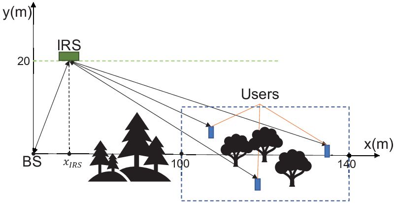
Refer to caption
Fig. 2: The simulated IRS-aided FD two-way multiuser communication scenario.

V-A Simulation Setup

Fig. 2 shows the horizontal plane of the schematic system model for our simulated network. As shown in the figure, we consider a system with K=3K=3 users, whose coordinates are generated uniformly and randomly in a rectangular region centered at (120,0)\left(120,0\right) with length 40 m and width 20 m. The coordinates of the BS and the IRS are (0,0)\left(0,0\right) and (xIRS,20)\left(x_{\rm IRS},20\right), respectively, where the default value of xIRSx_{\rm IRS} is 10. We assume that the height of the BS, the IRS, and the users are 30​m30\;\text{m}, 10​m10\;\text{m}, and 1.5​m1.5\;\text{m} [36], respectively.

The path loss is taken to be -30 dB at a reference distance of 1 m. The path loss exponents of the links between the BS and the IRS as well as those of the links between the IRS and the users are denoted by αBI\alpha_{\rm{BI}} and αIU\alpha_{\rm{IU}}, respectively. As we stated in Section II, there is no direct link between the BS and the users. On the contrary, through proper site selection, the transmission environment for the IRS-provided link can be nearly free-space. Hence, we set αBI=αIU=αIRS=2.2\alpha_{\rm{BI}}=\alpha_{\rm{IU}}=\alpha_{\rm{IRS}}=2.2 [36]. Then, the large-scale path loss in dB is modeled by

PL=−30−10​α​log10​d,{\rm{PL}}=-30-10\alpha{\log_{10}}d, (53)

where dd is the link distance beyond the 1 m reference. The small-scale fading is assumed to be Rician distributed, modeled by

𝐆~=κκ+1​𝐆~LoS+1κ+1​𝐆~NLoS,{\bf{\tilde{G}}}=\sqrt{\frac{\kappa}{{\kappa+1}}}{{\bf{\tilde{G}}}^{\rm{LoS}}}+\sqrt{\frac{1}{{\kappa+1}}}{{\bf{\tilde{G}}}^{\rm{NLoS}}}, (54)

where κ\kappa is the Rician factor, 𝐆~LoS{{\bf{\tilde{G}}}^{\rm{LoS}}} and 𝐆~NLoS{{\bf{\tilde{G}}}^{\rm{NLoS}}} are the LoS and the NLoS components, respectively. 𝐆~NLoS{{\bf{\tilde{G}}}^{\rm{NLoS}}} is drawn from a Rayleigh distribution, and 𝐆~LoS{{\bf{\tilde{G}}}^{\rm{LoS}}} is modeled as

𝐆~LoS=𝐜r​(ϑAoA)​𝐜tH​(ϑAoD).{{\bf{\tilde{G}}}^{\rm{LoS}}}={{\bf{c}}_{r}}\left({{\vartheta^{\rm{AoA}}}}\right){{\bf{c}}^{\rm H}_{t}}\left({{\vartheta^{\rm{AoD}}}}\right). (55)

In (55), 𝐜r​(ϑAoA){{\bf{c}}_{r}}\left({{\vartheta^{\rm{AoA}}}}\right) and 𝐜t​(ϑAoD){{\bf{c}}_{t}}\left({{\vartheta^{\rm{AoD}}}}\right) are respectively given by

𝐜r(ϑAoA)=[1,ejπsinϑAoA,…,ejπ(Wr−1)sinϑAoA]T,\displaystyle{{\bf{c}}_{r}}\left({{\vartheta^{\rm{AoA}}}}\right)={\left[{1,{e^{j\pi\sin{\vartheta^{\rm{AoA}}}}},\ldots,{e^{j\pi\left({{W_{r}}-1}\right)\sin{\vartheta^{\rm{AoA}}}}}}\right]^{\rm T}}, (56a)
𝐜t(ϑAoD)=[1,ejπsinϑAoD,…,ejπ(Wt−1)sinϑAoD]T,\displaystyle{{\bf{c}}_{t}}\left({{\vartheta^{\rm{AoD}}}}\right)={\left[{1,{e^{j\pi\sin{\vartheta^{\rm{AoD}}}}},\ldots,{e^{j\pi\left({{W_{t}}-1}\right)\sin{\vartheta^{\rm{AoD}}}}}}\right]^{\rm T}}, (56b)

where WrW_{\rm r} and WtW_{\rm t} denote the number of antennas/elements at the receiver side and transmitter side, respectively, ϑAoA{{\vartheta^{\rm{AoA}}}} and ϑAoD{{\vartheta^{\rm{AoD}}}} are the angle of arrival and departure, respectively. In the simulations, we independently and randomly generate ϑAoA{{\vartheta^{\rm{AoA}}}} and ϑAoD{{\vartheta^{\rm{AoD}}}} in the range of [0,2​π]\left[0,2\pi\right]. For simplicity, we set σU2=1.1​σB2\sigma_{{\rm{U}}}^{2}=1.1\sigma_{\rm B}^{2} and σD,k2=1.1​σk2,∀k\sigma_{{\rm{D}},k}^{2}=1.1\sigma_{k}^{2},\forall k. Unless otherwise stated, the other parameters are set as follows: Channel bandwidth 10 MHz, Rician factor κ=3\kappa=3, noise power density -174 dBm/Hz, SI coefficient ρS=1\rho_{\rm S}=1, weighting factors ωl,k=1,∀l,k\omega_{l,k}=1,\forall l,k, user transmit power Pk=50P_{k}=50 mW, ∀k\forall k, number of BS antennas Nt=Nr=4N_{\rm t}=N_{\rm r}=4, maximum BS transmit power Pmax=1​ WP_{\rm{max}}=1\text{ W}, number of IRS reflection elements M=16M=16, x-coordinate of IRS xIRS=10x_{\rm IRS}=10 m, initial smoothing parameter μ=5\mu=5, adjusting factor ι=1.02\iota=1.02, upper bound μm​a​x=500\mu_{\mathrm{m}ax}=500, error tolerance εe=10−6\varepsilon_{\rm e}=10^{-6}. The following results are obtained by averaging over 200 independent channel realizations. The reflection coefficient vector ϕ\bm{\phi} is initialized by uniformly and randomly selecting the phase shift of each reflection element in [0,2​π]\left[0,2\pi\right]. The precoding matrix 𝐅\bf F is initialized by extracting the real and imaginary parts of each element of 𝐅\bf F from an independent Gaussian distribution, and then scaling 𝐅\bf F to satisfy the equality in (3).

V-B Baseline Schemes

In our simulation, Problem (25) and the relaxed version of Problem (30) in Algorithm 1 are solved using the MOSEK solver [44]. In the remainder of this section, we denote the proposed Algorithm 1 by BCD-SOCP, and Algorithm 2 by BCD-MM. In order to analyze the performance of our proposed algorithms, we consider three baseline schemes:

  1. 1.

    Note that MOSEK solver can optimally solve the SOCP (25). To compare the performance of our proposed algorithms in solving quasi-SOCP, we design a benchmark algorithm SOCP+MM by replacing steps 4 to 9 of Algorithm 2 with step 5 of Algorithm 1.

  2. 2.

    To analyse the benefits of jointly optimizing the precoding matrix and the reflection coefficient vector, we consider the schemes in which only the former is optimized. Specifically, the steps that update the value of ϕ\bm{\phi} are skipped. We refer to implementing Algorithm 1 with random phase as BCD-SOCP, Rand. A similar definition holds for BCD-MM, Rand.

  3. 3.

    Since an IRS with arbitrarily tunable phase shifts is difficult to implement, we consider a more practical scenario involving 2-bit control of each IRS element (e.g., 4 possible phase shifts per element). Specifically, each element of the optimal reflection coefficient vector ϕopt{\bm{\phi}}^{\rm opt} obtained by BCD-SOCP, BCD-MM or SOCP+MM is converted to the following quantized value:

    ϕm2−bit=exp{argminθ|∠ϕmopt−θ|},m=1,…,M,\phi_{m}^{{\rm{2-bit}}}=\exp\left\{{\arg\min_{\theta}\left|{\angle\phi_{m}^{{\rm{opt}}}-\theta}\right|}\right\},m=1,\ldots,M, (57)

    where θ∈{0,π2,π,3​π2}\theta\in\left\{{0,\frac{\pi}{2},\pi,\frac{{3\pi}}{2}}\right\}. The corresponding 𝐅\bf F is then updated. The resulting algorithms are denoted as BCD-SOCP, 2 bit, BCD-MM, 2 bit and SOCP+MM, 2 bit, respectively.

V-C Convergence of Proposed Algorithm

Refer to caption
(a) Achievable WMR versus the number of iterations
Refer to caption
(b) Achievable WMR versus CPU time
Fig. 3: Convergence behaviour of proposed algorithms for M=[8,16]M=\left[8,16\right]

Fig. 3 plots the WMR versus the number of iterations and the CPU time for M=8​and​ 16M=8\;\text{and}\;16, illustrating the convergence behaviour of our proposed algorithms and the benchmark algorithm. 200 iterations of each algorithm are performed in each trial. We see that all the algorithms converge within 80 iterations, which confirms their high efficiency. The converged WMR of BCD-SOCP and BCD-MM are basically the same, and both are slightly lower than that of SOCP+MM, which shows the accuracy of MOSEK in solving SOCP and MM algorithm’s advantages in finding globally optimal solution of quasi-SOCP. However, due to its advantage in computational complexity, BCD-MM converges much faster in terms of CPU time. Additionally, it is interesting to observe that even when the number of reflection coefficients doubles, its convergence speed in terms of both number of iterations and CPU time does not increase significantly. The explanation can be found in the updating strategy for the smoothing factor and the computational complexity of the algorithms. On the one hand, the convergence speed of Algorithm 2 mainly depends on the approximation level of the surrogate functions in the MM iterations, which is mainly controlled by μ\mu, whose rate of increase is set to gradually accelerate. On the other hand, the quadratic and cubic terms in MM only account for less than half of the seven terms in the expression for the computational complexity of Algorithm 2 in (IV-C2). This indicates that our proposed Algorithm 2 will maintain good convergence performance and relatively low complexity even for the case of large MM.

V-D Impact of the IRS Location

Refer to caption
(a) Achievable WMR versus xIRSx_{\rm{IRS}} for ρS=1\rho_{S}=1.
Refer to caption
(b) Achievable WMR versus xIRSx_{\rm{IRS}} for ρS=0.1\rho_{S}=0.1.
Fig. 4: Impact of the IRS location xIRSx_{\rm{IRS}} and SI coefficient ρS\rho_{S}.

In order to provide engineering guidance for IRS site selection in practical communication systems, we investigate the effect of IRS location on the achievable WMR. By moving the IRS along the dotted line in Fig. 2 from xIRS=0x_{\rm{IRS}}=0 to xIRS=130x_{\rm{IRS}}=130, Fig. 4(a) and Fig. 4(b) illustrate the impact of IRS location on the achievable WMR for two cases of the SI coefficient ρS=1\rho_{S}=1 and ρS=0.1\rho_{S}=0.1, respectively. We can first draw a preliminary conclusion from these figures that for all eight schemes, IRS deployments nearer the BS improve the WMR. Second, recall that the x-coordinate of the users is distributed independently and uniformly between 100 and 140 in our simulation. Let us loosely name the point (120,0) as the user central point, and name the space on the left and right side of x=60x=60 as the BS side and the user side, respectively. Then, it can be observed that there are always two peaks in the achievable WMR for the various schemes, one on the BS side and one on the user side. Due to the increase in path loss, the achievable WMR decreases as expected when xIRSx_{\rm{IRS}} is too small or too large. Furthermore, the valley value of the WMR that occurs when xIRS≈60x_{\rm{IRS}}\approx 60 may also be explained by path loss. We can approximate the large-scale channel gain as follows

PLIRS=−60−10​α​log10⁡(xIRS)−10​α​log10⁡(xUEC−xIRS),\displaystyle{\rm{P}}{{\rm{L}}_{{\rm{IRS}}}}=-60-10\alpha{\log_{10}}\left({{x_{{\rm{IRS}}}}}\right)-10\alpha{\log_{10}}\left({{x_{{\rm{UEC}}}}-{x_{{\rm{IRS}}}}}\right), (58)

where xUEC{x_{{\rm{UEC}}}} denotes the x-coordinate of the user central point. Thus, the minimum value of (58) is achieved at xUEC∗=xIRS/2{x^{*}_{{\rm{UEC}}}}={x_{{\rm{IRS}}}}/2, which is consistent with the simulation results. Finally, as expected, the schemes that jointly optimize 𝐅\bf F and ϕ\bm{\phi} significantly improve the WMR performance over the Rand schemes. The performance of the 2 bit schemes with lower hardware cost falls in between the optimal continuous-phase and the random phase solutions, indicating that much improved performance can be obtained with even coarsely quantized phases.

V-E Impact of the SI Coefficient

Next we focus on the effect of SI in Fig. 4. Comparing Fig. 4(b) with Fig. 4(a), efficient user SI elimination techniques can improve the WMR when the IRS is deployed on the user side. Specifically, the achievable WMRs for BCD-MM and SOCP+MM schemes increase from 0.85 to 0.95 when xIRS=120x_{\rm{IRS}}=120. However, it should be emphasized that ρS=0.1\rho_{\rm S}=0.1 is an ideal case, the feasibility of which needs experimental verification in real scenarios. It can be observed that even in this ideal scenario, the WMR achieved by deploying the IRS near the users is still lower than when the IRS is deployed near the BS. This is due to the fact that there is also co-channel interference (CI) in the signals received by the users. When the IRS is further away from the users, the impact of both SI and CI is relatively small. Additionally, with an increase in number of users KK, CI gradually increases and becomes dominant. Thus, more of the IRS resources will be assigned to reduce the CI when it is deployed near the users.

V-F Impact of Asymmetric Priority

Refer to caption
Fig. 5: Impact of the IRS location xIRSx_{\rm{IRS}} for asymmetric-priority scenarios.

As mentioned in Remark 1, the desired uplink and downlink rates in a cellular system are often asymmetric. To provide more comprehensive engineering guidance, in Fig. 5, we set weighting factors ωU,k=ωU\omega_{{\rm U},k}=\omega_{{\rm U}} and ωD,k=ωD\omega_{{\rm D},k}=\omega_{{\rm D}} for ∀k\forall k and study achievable WMR versus xIRSx_{\rm{IRS}} in the following three scenarios various in priority condition: 1) Downlink first (ωU=2,ωD=1\omega_{{\rm U}}=2,\omega_{{\rm D}}=1, denoted as U2D1); 2) Equal priority (ωU=1,ωD=1\omega_{{\rm U}}=1,\omega_{{\rm D}}=1, denoted as U1D1); 3) Uplink first (ωU=1,ωD=2\omega_{{\rm U}}=1,\omega_{{\rm D}}=2, denoted as U1D2). BCD-MM is adopted in all schemes. It should be emphasized that the WMR, whose value is affected by the weighting factor, is not equivalent to the data rate. We see that for most scenarios, IRS is preferable to deployed on the BS side than on the user side. This contrast is obvious in the downlink first scenario, which is the most common in practice. A slightly different conclusion is presented only in uplink first scenarios where IRS has arbitrary phase shifts. Based on the discussions in this and the previous subsections, it can be concluded that in a common FD two-way communication scenario, the IRS deployment location that maximizes performance of all users is between the BS and users, near the BS. However, since the BS-to-user channels are blocked, moving the IRS closer to the BS may increase the likelihood that the IRS-to-user channels become blocked as well.

V-G Impact of the Weights and the Achieved Fairness

Refer to caption
Fig. 6: Individual data rate under two sets of weights.

As mentioned in the problem formulation, the essence of guaranteeing the fairness is to allocate resources from the users with higher rates to those with lower rates, thus the data rates of all users tend to be equal. Additionally, the weighting factor ωl,k\omega_{l,k} represents the inverse of the priority of the corresponding user in the link direction ll. This means that by appropriately setting ωl,k\omega_{l,k}, multiple user characteristics can be taken into account. To illustrate this, we choose an example with ωD,k=ωU,k\omega_{{\rm D},k}=\omega_{{\rm U},k} for each user, and set the coordinates of the three users as (100,10),(120,0)\left(100,10\right),\left(120,0\right) and (140,−10)\left(140,-10\right). Taking the user activity levels into consideration, two scenarios are tested: 1) Each user is active (ωk=1,∀k\omega_{k}=1,\forall k); and 2) User 2 is more active than the other two users (ω2=1,ω1=ω3=2\omega_{2}=1,\omega_{1}=\omega_{3}=2). Fig. 6 illustrates the individual data rates achieved under both scenarios. The average of the data rates is also plotted. As expected, a balanced rate distribution is obtained with equal weights, even though the path loss related to each user varies significantly. Additionally, the most active user 2 achieves the highest data rate in the scenario with different user activity levels. Furthermore, the essentially constant average rate illustrates the flexibility of the IRS-aided communication system for resource allocation.

V-H Impact of the Path Loss Exponent

Refer to caption
Fig. 7: Achievable WMR versus path loss exponent.

In some practical scenarios, an ideal location for deploying the IRS may be infeasible, which means that path loss exponents αIRS\alpha_{\rm{IRS}} as low as 2.2 may not be guaranteed. To investigate the system performance under different levels of fading, we plot Fig. 7 showing the achievable WMR for various path loss exponents. It can be observed that path loss has a significant impact on the WMR performance. Specifically, in each scenario, the increase in the achievable WMR is more than doubled for every 0.2 decrease in the value of αIRS\alpha_{\rm{IRS}}. Ultimately, the WMR performance decays to 0 at high values of αIRS\alpha_{\rm{IRS}}. This provides important guidance for engineering design: the performance gain obtained by deploying an IRS is greatly affected by channel conditions, thus the IRS should be deployed in a location with fewer obstacles.

V-I Impact of the Rician Factor

Refer to caption
Fig. 8: Achievable WMR versus the Rician factor.

Fig. 8 shows the achievable WMR for various Rician factors κ\kappa, which characterizes the scattering of the channel. As the multipath diversity gain decreases, the achievable WMR decreases as expected. Moreover, it can be observed that in the rich-scattering Rayleigh channel environment (κ=0\kappa=0), the achievable multipath diversity gain of the Rand schemes is significantly lower than that of the other methods, which again highlights the advantages of joint optimization.

V-J Impact of the Number of IRS Reflection Elements

Refer to caption
Fig. 9: Achievable WMR versus the number of IRS reflection elements MM.

According to the previous discussions, when the IRS is deployed on the BS side, doubling the number of its reflection elements MM can double the power of signals with little increase in interference and noise. Then, according to the Shannon formula, the channel capacity increases in an approximate logarithmic manner with the increase of MM. Fig. 9 shows the achievable WMR for various values of MM. As expected, the achievable WMR is not perfectly linear with the number of IRS reflection elements. The performance gain from increasing the elements decreases gradually. However, for the range of MM from 8 to 64, this decreasing trend is not very significant, indicating that it is cost-effective to improve communication performance by deploying more reflection elements.

VI Conclusions

In this paper, we have proposed a multiuser FD two-way communication network that exploits the availability of an IRS to enhance user fairness. Specifically, with appropriately adjusted phase shifts, the IRS can create effective reflective paths between the BS and the users, while simultaneously mitigating the interference at the users. We investigated the WMR maximization problem, where the BS precoding matrix and the IRS reflection coefficients were jointly optimized subject to maximum transmit power and unit-modulus constraints. We transformed the original problem into an equivalent form, and then introduced the BCD algorithm to alternately optimize the variables. An MM algorithm with closed-form solutions in each iteration was proposed to further reduce the computational complexity. Our simulation results showed that the proposed algorithm has a high convergence speed in terms of both the number of iterations and CPU time, and achieves high communication performance. In addition, the results imply that when the IRS is deployed near the users, user SI elimination techniques can improve system performance to some extent. But in common scenarios, the IRS should be deployed at a location between the BS and the users with favorable reflection links, closer to the BS.

Appendix A Proof of Theorem 1

Note that each hD,k​(𝐅),k∈𝒦{h_{{\rm{D}},k}}\left({\bf{F}}\right),{k\in{\cal K}} is a quadratic function, so we propose that the minorizing function for f⁡(𝐅)f\left({\bf{F}}\right) has the following quadratic form:

f~​(𝐅|𝐅n)\displaystyle\tilde{f}\left({{\bf{F}}|{{\bf{F}}^{n}}}\right) =f⁡(𝐅n)+2​Re{Tr[𝐃H​(𝐅−𝐅n)]}\displaystyle=f\left({{{\bf{F}}^{n}}}\right)+2{\mathop{\rm Re}\nolimits}\left\{{{\mathop{\rm Tr}\nolimits}\left[{{{\bf{D}}^{\rm H}}\left({{\bf{F}}-{{\bf{F}}^{n}}}\right)}\right]}\right\}
+Tr[(𝐅−𝐅n)H𝐌(𝐅−𝐅n)],\displaystyle\quad+{\mathop{\rm Tr}\nolimits}\left[{{{\left({{\bf{F}}-{{\bf{F}}^{n}}}\right)}^{\rm H}}{\bf{M}}\left({{\bf{F}}-{{\bf{F}}^{n}}}\right)}\right], (59)

where 𝐃∈ℂNt×Nt{\bf{D}}\in{\mathbb{C}}^{{N_{\rm t}}\times{N_{\rm t}}} and 𝐌∈ℂNt×Nt{\bf{M}}\in{\mathbb{C}}^{{N_{\rm t}}\times{N_{\rm t}}} are undetermined parameters. Note that conditions (A1) and (A4) are already satisfied, so the expressions for 𝐃\bf D and 𝐌\bf M are determined by conditions (A2) and (A3).

Let 𝐅t{\bf{F}}^{\rm t} be a member of 𝒮F{{\cal S}_{F}}. Then, the directional derivative of f~​(𝐅|𝐅n)\tilde{f}\left({{\bf{F}}|{{\bf{F}}^{n}}}\right) in (A) at 𝐅n{{\bf{F}}^{n}} in direction 𝐅t−𝐅n{\bf{F}}^{\rm t}-{{\bf{F}}^{n}} is given by

2​Re{Tr[𝐃H​(𝐅t−𝐅n)]}.2{\mathop{\rm Re}\nolimits}\left\{{{\mathop{\rm Tr}\nolimits}\left[{{{\bf{D}}^{\rm H}}\left({{\bf{F}}^{\rm t}-{{\bf{F}}^{n}}}\right)}\right]}\right\}. (60)

In addition, the directional derivative of f⁡(𝐅)f\left({\bf{F}}\right) is

2​Re{Tr[∑k∈𝒦gD,k​(𝐅n)​(𝐂kH−(𝐅n)H​𝐁k)​(𝐅t−𝐅n)]},2{\mathop{\rm Re}\nolimits}\left\{{{\mathop{\rm Tr}\nolimits}\left[{\sum\limits_{k\in{\cal K}}{{g_{{\rm{D}},k}}\left({{{\bf{F}}^{n}}}\right)\left({{\bf{C}}_{k}^{\rm H}-{{\left({{{\bf{F}}^{n}}}\right)}^{\rm H}}{{\bf{B}}_{k}}}\right)\left({{\bf{F}}^{\rm t}-{{\bf{F}}^{n}}}\right)}}\right]}\right\}, (61)

where gD,k​(𝐅n){g_{D,k}}\left({{{\bf{F}}^{n}}}\right) is defined in (40a). From condition (A3), the two directional derivatives (60) and (61) must be equal. By comparing the coefficients, the matrix 𝐃{\bf{D}} is identified as

𝐃=∑k∈𝒦gD,k​(𝐅n)​(𝐂k−𝐁kH​𝐅n).{\bf{D}}=\sum\limits_{k\in{\cal K}}{{g_{{\rm{D}},k}}\left({{{\bf{F}}^{n}}}\right)\left({{{\bf{C}}_{k}}-{\bf{B}}_{k}^{\rm H}{{\bf{F}}^{n}}}\right)}. (62)

Then, to satisfy condition (A2), we try to make the minorizing function f~​(𝐅|𝐅n)\tilde{f}\left({{\bf{F}}|{{\bf{F}}^{n}}}\right) be a lower bound of f⁡(𝐅)f\left({\bf{F}}\right) for each linear cut in any direction. By introducing an auxiliary variable η∈[0,1]\eta\in\left[0,1\right], and letting 𝐅=𝐅n+η⁡(𝐅t−𝐅n){\bf{F}}={{\bf{F}}^{n}}+\eta\left({{\bf{F}}^{\rm t}-{{\bf{F}}^{n}}}\right), this sufficient condition can be expressed as

f⁡(𝐅n+η⁡(𝐅t−𝐅n))\displaystyle f\left({{\bf{F}}^{n}}+\eta\left({{\bf{F}}^{\rm t}-{{\bf{F}}^{n}}}\right)\right)
≥f⁡(𝐅n)+2​η​Re{Tr[𝐃H​(𝐅t−𝐅n)]}\displaystyle\qquad\geq f\left({\bf{F}}^{n}\right)+2\eta{\mathop{\rm Re}\nolimits}\left\{{{\mathop{\rm Tr}\nolimits}\left[{{{\bf{D}}^{\rm H}}\left({{\bf{F}}^{\rm t}-{{\bf{F}}^{n}}}\right)}\right]}\right\}
+η2Tr[(𝐅t−𝐅n)H𝐌(𝐅t−𝐅n)].\displaystyle\qquad\quad+\eta^{2}{\mathop{\rm Tr}\nolimits}\left[{{{\left({{\bf{F}}^{\rm t}-{{\bf{F}}^{n}}}\right)}^{\rm H}}{\bf{M}}\left({{\bf{F}}^{\rm t}-{{\bf{F}}^{n}}}\right)}\right]. (63)

Denote the left and right hand side of (A) by jF​(η){j_{F}}\left(\eta\right) and JF​(η){J_{F}}\left(\eta\right), respectively. Then, it is apparent that jF​(0)=JF​(0){j_{F}}\left(0\right)={J_{F}}\left(0\right). The first-order derivative of jF​(η){j_{F}}\left(\eta\right) is calculated as

∇ηjF​(η)=∑k∈𝒦g^D,k​(η)​∇ηh^D,k​(η),{\nabla_{\eta}}{j_{F}}\left(\eta\right)=\sum\limits_{k\in{\cal K}}{{{\hat{g}}_{{\rm{D}},k}}\left(\eta\right){\nabla_{\eta}}{{\hat{h}}_{{\rm{D}},k}}\left(\eta\right)}, (64)

where

h^D,k​(η)=ΔhD,k​(𝐅n+η⁡(𝐅t−𝐅n)),\displaystyle{{\hat{h}}_{{\rm{D}},k}}\left(\eta\right)\mathrel{\mathop{\kern 0.0pt=}\limits^{\Delta}}{{{h}}_{{\rm{D}},k}}{\left({{\bf{F}}^{n}}+\eta\left({{\bf{F}}^{\rm t}-{{\bf{F}}^{n}}}\right)\right)}, (65a)
g^D,k​(η)=Δexp⁡{−μ​h^D,k​(η)}∑k∈𝒦exp⁡{−μ​h^D,k​(η)},k∈𝒦.\displaystyle{{\hat{g}}_{{\rm{D}},k}}\left(\eta\right)\mathrel{\mathop{\kern 0.0pt=}\limits^{\Delta}}\frac{{\exp\left\{{-\mu{{\hat{h}}_{{\rm{D}},k}}\left({\eta}\right)}\right\}}}{{\sum\limits_{k\in{\cal K}}{\exp\left\{{-\mu{{\hat{h}}_{{\rm{D}},k}}\left({\eta}\right)}\right\}}}},k\in{\cal K}. (65b)

And it can be derived that

∇ηh^D,k​(η)\displaystyle{\nabla_{\eta}}{\hat{h}_{{\rm{D}},k}}\left(\eta\right)
=2​R​e​{Tr⁡(𝐂kH​(𝐅t−𝐅n)−(𝐅n)H​𝐁k​(𝐅t−𝐅n))}\displaystyle=2{\rm{Re}}\left\{{{\rm{Tr}}\left({{\bf{C}}_{k}^{\rm{H}}\left({{{\bf{F}}^{\rm{t}}}-{{\bf{F}}^{n}}}\right)-{{\left({{{\bf{F}}^{n}}}\right)}^{\rm{H}}}{{\bf{B}}_{k}}\left({{{\bf{F}}^{\rm{t}}}-{{\bf{F}}^{n}}}\right)}\right)}\right\}
−2​η​Tr​((𝐅t−𝐅n)H​𝐁k​(𝐅t−𝐅n)).\displaystyle\quad-2\eta{\rm{Tr}}\left({{{\left({{{\bf{F}}^{\rm{t}}}-{{\bf{F}}^{n}}}\right)}^{\rm{H}}}{{\bf{B}}_{k}}\left({{{\bf{F}}^{\rm{t}}}-{{\bf{F}}^{n}}}\right)}\right). (66)

It is readily verified that ∇ηjF​(0)=∇ηJF​(0){\nabla_{\eta}}{j_{F}}\left(0\right)={\nabla_{\eta}}{J_{F}}\left(0\right). Then, since JF​(η){J_{F}}\left(\eta\right) is concave w.r.t. η\eta, a sufficient condition for (A) to hold is that the second-order derivative of jF​(η){j_{F}}\left(\eta\right) is greater than or equal to that of JF​(η){J_{F}}\left(\eta\right) for ∀η∈[0,1]\forall\eta\in\left[0,1\right], i.e.

∇η2​jF​(η)≥∇η2​JF​(η),∀η∈[0,1].\nabla_{\eta}^{2}{j_{F}}\left(\eta\right)\geq\nabla_{\eta}^{2}{J_{F}}\left(\eta\right),\forall\eta\in\left[0,1\right]. (67)

In the following, we compute the second-order derivative of jF​(η){j_{F}}\left(\eta\right) to determine the value of 𝐌{\bf{M}}. First, by defining

𝐄k=Δ𝐂k−𝐁kH​(𝐅n+η⁡(𝐅t−𝐅n)),{\bf{E}}_{k}\mathrel{\mathop{\kern 0.0pt=}\limits^{\Delta}}{{\bf{C}}_{k}}-{\bf{B}}_{k}^{\rm H}\left({{{\bf{F}}^{n}}+\eta\left({{{\bf{F}}^{t}}-{{\bf{F}}^{n}}}\right)}\right),

(A) can be rewritten as

∇ηh^D,k​(η)\displaystyle{\nabla_{\eta}}{\hat{h}_{{\rm{D}},k}}\left(\eta\right) =2​R​e​{Tr⁡(𝐄kH​(𝐅t−𝐅n))}\displaystyle=2{\rm{Re}}\left\{{{\rm{Tr}}\left({{\bf{E}}_{k}^{\rm{H}}\left({{{\bf{F}}^{t}}-{{\bf{F}}^{n}}}\right)}\right)}\right\}
=2​Re{𝐞kH​𝐟¯},\displaystyle=2{\mathop{\rm Re}\nolimits}\left\{{{\bf{e}}_{k}^{\rm H}{\bf{\bar{f}}}}\right\}, (68)

where 𝐞k=Δvec(𝐄k){{\bf{e}}_{k}}\mathrel{\mathop{\kern 0.0pt=}\limits^{\Delta}}{\mathop{\rm vec}\nolimits}\left({{{\bf{E}}_{k}}}\right) and 𝐟¯=Δvec(𝐅t−𝐅n){{\bf{\bar{f}}}}\mathrel{\mathop{\kern 0.0pt=}\limits^{\Delta}}{\mathop{\rm vec}\nolimits}\left({{{\bf{F}}^{t}}-{{\bf{F}}^{n}}}\right). The second-order derivative of h^D,k​(η){\hat{h}_{{\rm{D}},k}}\left(\eta\right) is given by

∇η2​h^D,k​(η)\displaystyle\nabla_{\eta}^{2}{\hat{h}_{D,k}}\left(\eta\right) =−2Tr((𝐅t−𝐅n)H𝐁k(𝐅t−𝐅n))\displaystyle=-2{\mathop{\rm Tr}\nolimits}\left({{{\left({{{\bf{F}}^{t}}-{{\bf{F}}^{n}}}\right)}^{\rm{H}}}{{\bf{B}}_{k}}\left({{{\bf{F}}^{t}}-{{\bf{F}}^{n}}}\right)}\right)
=−2​𝐟¯H​(𝐈⊗𝐁k)​𝐟¯,\displaystyle=-2{{\bf{\bar{f}}}^{\rm H}}\left({{\bf{I}}\otimes{{\bf{B}}_{k}}}\right){\bf{\bar{f}}}, (69)

where we have used the property that Tr(𝐀𝐁𝐂)=vecT(𝐀T)​(𝐈⊗𝐁)​vec(𝐂){\mathop{\rm Tr}\nolimits}\left({{\bf{ABC}}}\right)={{\mathop{\rm vec}\nolimits}^{\rm T}}\left({{{\bf{A}}^{\rm T}}}\right)\left({{\bf{I}}\otimes{\bf{B}}}\right){\mathop{\rm vec}\nolimits}\left({\bf{C}}\right) [37]. Then, the second-order derivative of jF​(η){j_{F}}\left(\eta\right) is derived as

∇η2​jF​(η)\displaystyle\nabla_{\eta}^{2}{j_{F}}\left(\eta\right)
=∑k∈𝒦(g^D,k​(η)​∇η2h^D,k​(η)−μ​g^D,k​(η)​(∇ηh^D,k​(η))2)\displaystyle=\sum\limits_{k\in{\cal K}}{\left({{{\hat{g}}_{{\rm{D}},k}}\left(\eta\right)\nabla_{\eta}^{2}{{\hat{h}}_{{\rm{D}},k}}\left(\eta\right)-\mu{{\hat{g}}_{{\rm{D}},k}}\left(\eta\right){{\left({{\nabla_{\eta}}{{\hat{h}}_{{\rm{D}},k}}\left(\eta\right)}\right)}^{2}}}\right)}\quad
+μ​(∑k∈𝒦g^D,k​(η)​∇ηh^D,k​(η))2\displaystyle\quad+\mu{\left({\sum\limits_{k\in{\cal K}}{{{\hat{g}}_{{\rm{D}},k}}\left(\eta\right){\nabla_{\eta}}{{\hat{h}}_{{\rm{D}},k}}\left(\eta\right)}}\right)^{2}}
=[𝐟¯H𝐟¯T]​Ξ​[𝐟¯𝐟¯∗],\displaystyle=\left[{\begin{array}[]{*{20}{c}}{{{{\bf{\bar{f}}}}^{\rm H}}}&{{{{\bf{\bar{f}}}}^{\rm T}}}\end{array}}\right]\Xi\left[{\begin{array}[]{*{20}{c}}{{\bf{\bar{f}}}}\\ {{{{\bf{\bar{f}}}}^{*}}}\end{array}}\right],

where Ξ\Xi is given by (73) on the top of the next page.

𝚵=−∑k∈𝒦g^D,k(η)([𝐈⊗𝐁k𝟎𝟎𝐈⊗𝐁kH]+μ[𝐞k𝐞k∗][𝐞k𝐞k∗]H)+μ[∑k∈𝒦g^D,k​(η)​𝐞k∑k∈𝒦g^D,k​(η)​𝐞k∗][∑k∈𝒦g^D,k​(η)​𝐞k∑k∈𝒦g^D,k​(η)​𝐞k∗]H.{\bf{\Xi}}=-\sum\limits_{k\in{\cal K}}{{{\hat{g}}_{{\rm{D}},k}}\left(\eta\right)\left({\left[{\begin{array}[]{*{20}{c}}{{\bf{I}}\otimes{{\bf{B}}_{k}}}&{\bf{0}}\\ {\bf{0}}&{{\bf{I}}\otimes{\bf{B}}_{k}^{\rm H}}\end{array}}\right]+\mu\left[{\begin{array}[]{*{20}{c}}{{{\bf{e}}_{k}}}\\ {{\bf{e}}_{k}^{*}}\end{array}}\right]{{\left[{\begin{array}[]{*{20}{c}}{{{\bf{e}}_{k}}}\\ {{\bf{e}}_{k}^{*}}\end{array}}\right]}^{\rm H}}}\right)}+\mu\left[{\begin{array}[]{*{20}{c}}{\sum\limits_{k\in{\cal K}}{{{\hat{g}}_{D,k}}\left(\eta\right){{\bf{e}}_{k}}}}\\ {\sum\limits_{k\in{\cal K}}{{{\hat{g}}_{D,k}}\left(\eta\right){\bf{e}}_{k}^{*}}}\end{array}}\right]{\left[{\begin{array}[]{*{20}{c}}{\sum\limits_{k\in{\cal K}}{{{\hat{g}}_{D,k}}\left(\eta\right){{\bf{e}}_{k}}}}\\ {\sum\limits_{k\in{\cal K}}{{{\hat{g}}_{D,k}}\left(\eta\right){\bf{e}}_{k}^{*}}}\end{array}}\right]^{\rm H}}. (73)


We also compute the second-order derivative of ∇η2​JF​(η)\nabla_{\eta}^{2}{J_{F}}\left(\eta\right), and manipulate it into a quadratic form, as follows

∇η2​JF​(η)\displaystyle\nabla_{\eta}^{2}{J_{F}}\left(\eta\right) =2​Tr[(𝐅t−𝐅n)H​𝐌​(𝐅t−𝐅n)]\displaystyle=2{\mathop{\rm Tr}\nolimits}\left[{{{\left({{\bf{F}}^{\rm t}-{{\bf{F}}^{n}}}\right)}^{\rm H}}{\bf{M}}\left({{\bf{F}}^{\rm t}-{{\bf{F}}^{n}}}\right)}\right]
=[𝐟¯H𝐟¯T]​[𝐈⊗𝐌𝟎𝟎𝐈⊗𝐌T]​[𝐟¯𝐟¯∗].\displaystyle=\left[{\begin{array}[]{*{20}{c}}{{{{\bf{\bar{f}}}}^{\rm H}}}&{{{{\bf{\bar{f}}}}^{\rm T}}}\end{array}}\right]\left[{\begin{array}[]{*{20}{c}}{{\bf{I}}\otimes{\bf{M}}}&{\bf{0}}\\ {\bf{0}}&{{\bf{I}}\otimes{{\bf{M}}^{\rm T}}}\end{array}}\right]\left[{\begin{array}[]{*{20}{c}}{{\bf{\bar{f}}}}\\ {{{{\bf{\bar{f}}}}^{*}}}\end{array}}\right].

Then, the inequality in (67) is reformulated as

[𝐟¯H𝐟¯T]​𝚵​[𝐟¯𝐟¯∗]\displaystyle\left[{\begin{array}[]{*{20}{c}}{{{{\bf{\bar{f}}}}^{\rm H}}}&{{{{\bf{\bar{f}}}}^{\rm T}}}\end{array}}\right]{\bf{\Xi}}\left[{\begin{array}[]{*{20}{c}}{{\bf{\bar{f}}}}\\ {{{{\bf{\bar{f}}}}^{*}}}\end{array}}\right]
≥[𝐟¯H𝐟¯T]​[𝐈⊗𝐌𝟎𝟎𝐈⊗𝐌T]​[𝐟¯𝐟¯∗].\displaystyle\qquad\geq\left[{\begin{array}[]{*{20}{c}}{{{{\bf{\bar{f}}}}^{\rm H}}}&{{{{\bf{\bar{f}}}}^{\rm T}}}\end{array}}\right]\left[{\begin{array}[]{*{20}{c}}{{\bf{I}}\otimes{\bf{M}}}&{\bf{0}}\\ {\bf{0}}&{{\bf{I}}\otimes{{\bf{M}}^{\rm T}}}\end{array}}\right]\left[{\begin{array}[]{*{20}{c}}{{\bf{\bar{f}}}}\\ {{{{\bf{\bar{f}}}}^{*}}}\end{array}}\right].

As a result, 𝐌{\bf{M}} must satisfy

𝚵⪰[𝐈⊗𝐌𝟎𝟎𝐈⊗𝐌T].{\bf{\Xi}}\succeq\left[{\begin{array}[]{*{20}{c}}{{\bf{I}}\otimes{\bf{M}}}&{\bf{0}}\\ {\bf{0}}&{{\bf{I}}\otimes{{\bf{M}}^{\rm T}}}\end{array}}\right]. (87)

We choose the following simple solution: 𝐌=α​𝐈=λmin​(𝚵)​𝐈{\bf{M}}=\alpha{\bf{I}}={\lambda_{\min}}\left({\bf{\Xi}}\right){\bf{I}}. Then, (A) is equivalent to

f~​(𝐅|𝐅n)\displaystyle\tilde{f}\left({{\bf{F}}|{{\bf{F}}^{n}}}\right) =f⁡(𝐅n)+2​Re{Tr[𝐃H​(𝐅−𝐅n)]}\displaystyle=f\left({{{\bf{F}}^{n}}}\right)+2{\mathop{\rm Re}\nolimits}\left\{{{\mathop{\rm Tr}\nolimits}\left[{{{\bf{D}}^{\rm H}}\left({{\bf{F}}-{{\bf{F}}^{n}}}\right)}\right]}\right\}
+αTr[(𝐅−𝐅n)H(𝐅−𝐅n)]\displaystyle\quad+\alpha{\mathop{\rm Tr}\nolimits}\left[{{{\left({{\bf{F}}-{{\bf{F}}^{n}}}\right)}^{\rm H}}\left({{\bf{F}}-{{\bf{F}}^{n}}}\right)}\right]
=2​Re{Tr[𝐕H​𝐅]}+α​Tr[𝐅H​𝐅]+cons​F,\displaystyle={2{\mathop{\rm Re}\nolimits}\left\{{{\mathop{\rm Tr}\nolimits}\left[{{{\bf{V}}^{\rm H}}{\bf{F}}}\right]}\right\}+\alpha{\mathop{\rm Tr}\nolimits}\left[{{{\bf{F}}^{\rm H}}{\bf{F}}}\right]+{\rm{cons}}F}, (88)

where 𝐕{\bf{V}} and cons​F{\rm{cons}}F are given in (39a) and (39b), respectively. However, 𝚵{\bf{\Xi}} is a very complex function w.r.t. η\eta, which leads to a high computation cost to calculate α\alpha in (A). To reduce the complexity, we proceed to find a simple lower bound to replace α\alpha, as shown in (A) on the top of the next page,

α=λmin​(𝚵)\displaystyle\alpha={\lambda_{\min}}\left({\bf{\Xi}}\right) ≥(a​1)−∑k∈𝒦g^D,k​(η)​(λmax​([𝐈⊗𝐁k𝟎𝟎𝐈⊗𝐁kH])+μ​λmax​([𝐞k𝐞k∗]​[𝐞k𝐞k∗]H))\displaystyle\overset{(a1)}{\geq}-\sum\limits_{k\in{\cal K}}{{{\hat{g}}_{{\rm{D}},k}}\left(\eta\right)\left({{\lambda_{\max}}\left({\left[{\begin{array}[]{*{20}{c}}{{\bf{I}}\otimes{{\bf{B}}_{k}}}&{\bf{0}}\\ {\bf{0}}&{{\bf{I}}\otimes{\bf{B}}_{k}^{\rm{H}}}\end{array}}\right]}\right)+\mu{\lambda_{\max}}\left({\left[{\begin{array}[]{*{20}{c}}{{{\bf{e}}_{k}}}\\ {{\bf{e}}_{k}^{*}}\end{array}}\right]{{\left[{\begin{array}[]{*{20}{c}}{{{\bf{e}}_{k}}}\\ {{\bf{e}}_{k}^{*}}\end{array}}\right]}^{\rm{H}}}}\right)}\right)}
+μ​λmin​([∑k∈𝒦g^D,k​(η)​𝐞k∑k∈𝒦g^D,k​(η)​𝐞k∗]​[∑k∈𝒦g^D,k​(η)​𝐞k∑k∈𝒦g^D,k​(η)​𝐞k∗]H)\displaystyle\qquad+\mu{\lambda_{\min}}\left({\left[{\begin{array}[]{*{20}{c}}{\sum\limits_{k\in{\cal K}}{{{\hat{g}}_{{\rm{D}},k}}\left(\eta\right){{\bf{e}}_{k}}}}\\ {\sum\limits_{k\in{\cal K}}{{{\hat{g}}_{{\rm{D}},k}}\left(\eta\right){\bf{e}}_{k}^{*}}}\end{array}}\right]{{\left[{\begin{array}[]{*{20}{c}}{\sum\limits_{k\in{\cal K}}{{{\hat{g}}_{{\rm{D}},k}}\left(\eta\right){{\bf{e}}_{k}}}}\\ {\sum\limits_{k\in{\cal K}}{{{\hat{g}}_{{\rm{D}},k}}\left(\eta\right){\bf{e}}_{k}^{*}}}\end{array}}\right]}^{\rm{H}}}}\right)
=(a​2)−∑k∈𝒦g^D,k​(η)​(λmax​(𝐁k)+2​μ​𝐞kH​𝐞k)\displaystyle\overset{(a2)}{=}-\sum\limits_{k\in{\cal K}}{{{\hat{g}}_{{\rm{D}},k}}\left(\eta\right)\left({{\lambda_{\max}}\left({{{\bf{B}}_{k}}}\right)+2\mu{\bf{e}}_{k}^{\rm H}{{\bf{e}}_{k}}}\right)}
=(a​2)−∑k∈𝒦g^D,k​(η)​(tp1k)−2​μ​∑k∈𝒦g^D,k​(η)​‖𝐄k‖F2\displaystyle\overset{(a2)}{=}-\sum\limits_{k\in{\cal K}}{{{\hat{g}}_{{\rm{D}},k}}\left(\eta\right)\left({\rm{tp1}}_{k}\right)}-2\mu\sum\limits_{k\in{\cal K}}{{{\hat{g}}_{{\rm{D}},k}}\left(\eta\right)\left\|{{{\bf{E}}_{k}}}\right\|_{F}^{2}}
≥(a​3)−maxk{tp1k}−2​μ​maxk{‖𝐄k‖F2},\displaystyle\overset{(a3)}{\geq}-\mathop{\max}\limits_{k}\left\{{\rm{tp1}}_{k}\right\}-2\mu\mathop{\max}\limits_{k}\left\{{\left\|{{{\bf{E}}_{k}}}\right\|_{F}^{2}}\right\}, (99)


where tp1k{{\rm{tp1}}_{k}} is defined in (40c), and we have used the following properties (a1)-(a3):

  1. (a1)

    λmin​(𝐀)+λmin​(𝐁)≤λmin​(𝐀+𝐁){\lambda_{\min}}\left({\bf{A}}\right)+{\lambda_{\min}}\left({\bf{B}}\right)\leq{\lambda_{\min}}\left({{\bf{A}}+{\bf{B}}}\right), if 𝐀{\bf{A}} and 𝐁{\bf{B}} are Hermitian matrices [45];

  2. (a2)

    λmax​(𝐀)=Tr(𝐀){\lambda_{\max}}\left({\bf{A}}\right)={\mathop{\rm Tr}\nolimits}\left({\bf{A}}\right) and λmin​(𝐀)=0{\lambda_{\min}}\left({\bf{A}}\right)=0, if 𝐀{\bf{A}} is rank one [45];

  3. (a3)

    ∑m=1Mam​bm≤maxm=1M​{bm}\sum\nolimits_{m=1}^{M}{{a_{m}}{b_{m}}}\leq\max_{m=1}^{M}\left\{{{b_{m}}}\right\}, if am,bm≥0{a_{m}},{b_{m}}\geq 0 and ∑m=1Mam=1\sum\nolimits_{m=1}^{M}{{a_{m}}}=1 [46, Theorem 30].

Recall that 𝐅=𝐅n+η⁡(𝐅t−𝐅n){\bf{F}}={{\bf{F}}^{n}}+\eta\left({{\bf{F}}^{t}-{{\bf{F}}^{n}}}\right), thus the inequality ‖𝐅n+η⁡(𝐅t−𝐅n)‖F≤Pmax\left\|{{{\bf{F}}^{n}}+\eta\left({{{\bf{F}}^{t}}-{{\bf{F}}^{n}}}\right)}\right\|_{F}\leq\sqrt{P_{\max}} holds. Then an upper bound for ‖𝐄k‖F2\left\|{{{\bf{E}}_{k}}}\right\|_{F}^{2} is derived in (A) on the top of the next page,

‖𝐄k‖F2\displaystyle\left\|{{{\bf{E}}_{k}}}\right\|_{F}^{2} =‖𝐂k−𝐁kH​(𝐅n+η⁡(𝐅t−𝐅n))‖F2\displaystyle=\left\|{{{\bf{C}}_{k}}-{\bf{B}}_{k}^{\rm{H}}\left({{{\bf{F}}^{n}}+\eta\left({{{\bf{F}}^{t}}-{{\bf{F}}^{n}}}\right)}\right)}\right\|_{F}^{2}
=‖𝐁kH​(𝐅n+η⁡(𝐅t−𝐅n))‖F2+‖𝐂k‖F2−2​Re{Tr(𝐂kH​𝐁kH​(𝐅n+η⁡(𝐅t−𝐅n)))}\displaystyle=\left\|{{\bf{B}}_{k}^{\rm{H}}\left({{{\bf{F}}^{n}}+\eta\left({{{\bf{F}}^{t}}-{{\bf{F}}^{n}}}\right)}\right)}\right\|_{F}^{2}+\left\|{{{\bf{C}}_{k}}}\right\|_{F}^{2}-2{\mathop{\rm Re}\nolimits}\left\{{{\mathop{\rm Tr}\nolimits}\left({{\bf{C}}_{k}^{\rm H}{\bf{B}}_{k}^{\rm{H}}\left({{{\bf{F}}^{n}}+\eta\left({{{\bf{F}}^{t}}-{{\bf{F}}^{n}}}\right)}\right)}\right)}\right\}
≤(a​4)​λmax​(𝐁kH​𝐁k)​‖𝐅n+η⁡(𝐅t−𝐅n)‖F2+‖𝐂k‖F2−2​Re{Tr(𝐂kH​𝐁kH​(𝐅n+η⁡(𝐅t−𝐅n)))}\displaystyle\overset{(a4)}{\leq}{\lambda_{\max}}\left({{\bf{B}}_{k}^{\rm{H}}{{\bf{B}}_{k}}}\right)\left\|{{{\bf{F}}^{n}}+\eta\left({{{\bf{F}}^{t}}-{{\bf{F}}^{n}}}\right)}\right\|_{F}^{2}+\left\|{{{\bf{C}}_{k}}}\right\|_{F}^{2}-2{\mathop{\rm Re}\nolimits}\left\{{{\mathop{\rm Tr}\nolimits}\left({{\bf{C}}_{k}^{\rm H}{\bf{B}}_{k}^{\rm{H}}\left({{{\bf{F}}^{n}}+\eta\left({{{\bf{F}}^{t}}-{{\bf{F}}^{n}}}\right)}\right)}\right)}\right\}
≤(a​5)​Pmax​λmax​(𝐁kH​𝐁k)+‖𝐂k‖F2+2​Pmax​‖𝐁k​𝐂k‖F\displaystyle\overset{(a5)}{\leq}{P_{\max}}{\lambda_{\max}}\left({{\bf{B}}_{k}^{\rm{H}}{{\bf{B}}_{k}}}\right)+\left\|{{{\bf{C}}_{k}}}\right\|_{F}^{2}+2\sqrt{{P_{\max}}}{\left\|{{{\bf{B}}_{k}}{{\bf{C}}_{k}}}\right\|_{F}}
=(a​2)​Pmax​tp1k2+‖𝐂k‖F2+2​Pmax​‖𝐁k​𝐂k‖F.\displaystyle\overset{(a2)}{=}{P_{\max}}{\rm{tp1}}_{k}^{2}+\left\|{{{\bf{C}}_{k}}}\right\|_{F}^{2}+2\sqrt{{P_{\max}}}{\left\|{{{\bf{B}}_{k}}{{\bf{C}}_{k}}}\right\|_{F}}. (100)


where (a4) and (a5) are given by

  1. (a4)

    Tr(𝐀𝐁)≤λmax​(𝐀)​Tr(𝐁){\mathop{\rm Tr}\nolimits}\left({{\bf{AB}}}\right)\leq{\lambda_{\max}}\left({\bf{A}}\right){\mathop{\rm Tr}\nolimits}\left({\bf{B}}\right), if 𝐀\bf A and 𝐁\bf B are positive semidefinite matrices [45];

  2. (a5)

    −Pmax​‖𝐁𝐂‖F-\sqrt{{P_{\max}}}{\left\|{{{\bf{B}}}{{\bf{C}}}}\right\|_{F}} is the optimal value of the following Problem (101):

    min𝐗\displaystyle\min_{\bf{X}}\quad Re{Tr(𝐂H​𝐁H​𝐗)}\displaystyle{\mathop{\rm Re}\nolimits}\left\{{{\mathop{\rm Tr}\nolimits}\left({{{\bf{C}}^{\rm H}}{{\bf{B}}^{\rm H}}{\bf{X}}}\right)}\right\} (101a)
    s.t. Tr(𝐗H​𝐗)≤Pmax.\displaystyle{\mathop{\rm Tr}\nolimits}\left({{{\bf{X}}^{\rm H}}{\bf{X}}}\right)\leq{P_{\max}}. (101b)

Finally, by substituting (A) into (A), we arrive at (38). Hence, the proof is complete.

Appendix B Proof of Theorem 2

We propose a quadratic function to minorize f⁡(ϕ)f\left({\bm{\phi}}\right). Defining undetermined parameters 𝐍∈ℂM×M{\bf{N}}\in{\mathbb{C}}^{{M}\times{M}} and 𝐝∈ℂM×1{\bf{d}}\in{\mathbb{C}}^{{M}\times{1}}, the minorizing function f~​(ϕ|ϕn)\tilde{f}\left({{\bm{\phi}}|{{\bm{\phi}}^{n}}}\right) can be expressed as

f~​(ϕ|ϕn)\displaystyle\tilde{f}\left({{\bm{\phi}}|{{\bm{\phi}}^{n}}}\right) =f⁡(ϕn)+2​R​e​{𝐝H​(ϕ−ϕn)}\displaystyle=f\left({{{\bm{\phi}}^{n}}}\right)+2{\rm{Re}}\left\{{{{\bf{d}}^{\rm{H}}}\left({{\bm{\phi}}-{{\bm{\phi}}^{n}}}\right)}\right\}
+(ϕ−ϕn)H​𝐍​(ϕ−ϕn).\displaystyle\quad+{\left({{\bm{\phi}}-{{\bm{\phi}}^{n}}}\right)^{\rm{H}}}{\bf{N}}\left({{\bm{\phi}}-{{\bm{\phi}}^{n}}}\right). (102)

Since conditions (B1) and (B4) are already satisfied, in the following, we determine expressions for 𝐍{\bf{N}} and 𝐝{\bf{d}} to satisfy (B2) and (B3).

Beginning with (B3), the directional derivative of f~​(ϕ|ϕn)\tilde{f}\left({{\bm{\phi}}|{{\bm{\phi}}^{n}}}\right) at ϕn{{\bm{\phi}}^{n}} with direction (ϕt−ϕn)\left({\bm{\phi}}^{\rm t}-{\bm{\phi}}^{n}\right) is

2​Re​{𝐝H​(ϕt−ϕn)},2{\rm{Re}}\left\{{{{\bf{d}}^{\rm{H}}}\left({{\bm{\phi}}^{\rm t}-{{\bm{\phi}}^{n}}}\right)}\right\}, (103)

where ϕt∈𝒮ϕ{\bm{\phi}}^{\rm t}\in{\cal S}_{\phi}. Applying (B3), the directional derivative of f⁡(ϕ)f\left({\bm{\phi}}\right) must be equal to the directional derivative (103), which means

𝐝=∑l∈ℒ∑k∈𝒦gl,k​(ϕn)​(𝐚l,k−𝐀l,kH​ϕn),{\bf{d}}=\sum\limits_{l\in{\cal L}}{\sum\limits_{k\in{\cal K}}{{g_{l,k}}\left({\bm{\phi}}^{n}\right)\left({{{\bf{a}}_{l,k}}-{\bf{A}}_{l,k}^{\rm H}{{\bm{\phi}}^{n}}}\right)}}, (104)

where gl,k​(ϕn){g_{l,k}}\left({\bm{\phi}}^{n}\right) is defined in (49b).

Now we consider condition (B2). Let ϕ=ϕn+η⁡(ϕt−ϕn){\bm{\phi}}={\bm{\phi}}^{n}+\eta\left({\bm{\phi}}^{\rm t}-{\bm{\phi}}^{n}\right) with η∈[0,1]\eta\in\left[0,1\right]. Then a sufficient condition for (B2) is given by

f⁡(ϕn+η⁡(ϕt−ϕn))\displaystyle f\left({{{\bm{\phi}}^{n}}+\eta\left({{{\bm{\phi}}^{\rm t}}-{{\bm{\phi}}^{n}}}\right)}\right) ≥f⁡(ϕn)+2​η​Re​{𝐝H​(ϕt−ϕn)}\displaystyle\geq f\left({{{\bm{\phi}}^{n}}}\right)+2\eta{\rm{Re}}\left\{{{{\bf{d}}^{\rm{H}}}\left({{{\bm{\phi}}^{\rm t}}-{{\bm{\phi}}^{n}}}\right)}\right\}
+η2​(ϕt−ϕn)H​𝐍​(ϕt−ϕn).\displaystyle\quad+{\eta^{2}}{\left({{{\bm{\phi}}^{\rm t}}-{{\bm{\phi}}^{n}}}\right)^{\rm{H}}}{\bf{N}}\left({{{\bm{\phi}}^{\rm t}}-{{\bm{\phi}}^{n}}}\right). (105)

Denote the left and right hand side of (B) by jϕ​(η){j_{\phi}}\left(\eta\right) and Jϕ​(η){J_{\phi}}\left(\eta\right), respectively. Then we have jϕ​(0)=Jϕ​(0){j_{\phi}}\left(0\right)={J_{\phi}}\left(0\right) and ∇ηjϕ​(0)=∇ηJϕ​(0){\nabla_{\eta}}{j_{\phi}}\left(0\right)={\nabla_{\eta}}{J_{\phi}}\left(0\right). Since Jϕ{J_{\phi}} is concave w.r.t. η\eta, a sufficient condition for (B) to hold is

∇η2​jϕ​(η)≥∇η2​Jϕ​(η).\nabla_{\eta}^{2}{j_{\phi}}\left(\eta\right)\geq\nabla_{\eta}^{2}{J_{\phi}}\left(\eta\right). (106)

With the definition ϕ¯=Δϕt−ϕn{\bar{\bm{\phi}}}\mathrel{\mathop{\kern 0.0pt=}\limits^{\Delta}}{{{\bm{\phi}}^{\rm t}}-{{\bm{\phi}}^{n}}}, the second-order derivative of jϕ​(η){j_{\phi}}\left(\eta\right) is given by

∇η2​jϕ​(η)=[ϕ¯Hϕ¯T]​𝛀​[ϕ¯ϕ¯∗],\nabla_{\eta}^{2}{j_{\phi}}\left(\eta\right)=\left[{\begin{array}[]{*{20}{c}}{{\bar{\bm{\phi}}^{\rm H}}}&{{\bar{\bm{\phi}}^{\rm T}}}\end{array}}\right]{\bf\Omega}\left[{\begin{array}[]{*{20}{c}}\bar{\bm{\phi}}\\ {{\bar{\bm{\phi}}^{*}}}\end{array}}\right], (107)

where 𝛀{\bf{\Omega}} is given in (108) on the top of the next page.

𝛀=−∑l∈ℒ∑k∈𝒦g^l,k(η)([𝐀l,k𝟎𝟎𝐀l,kT]+μ[𝐮l,k𝐮l,k∗][𝐮l,k𝐮l,k∗]H)+μ[∑l∈ℒ∑k∈𝒦g^l,k​(η)​𝐮l,k∑l∈ℒ∑k∈𝒦g^l,k​(η)​𝐮l,k∗][∑l∈ℒ∑k∈𝒦g^l,k​(η)​𝐮l,k∑l∈ℒ∑k∈𝒦g^l,k​(η)​𝐮l,k∗]H.\begin{split}&{\bf{\Omega}}=-\sum\limits_{l\in{\cal L}}{\sum\limits_{k\in{\cal K}}{{{\hat{g}}_{l,k}}\left(\eta\right)\left({\left[{\begin{array}[]{*{20}{c}}{{{\bf{A}}_{l,k}}}&{\bf{0}}\\ {\bf{0}}&{{\bf{A}}_{l,k}^{\rm T}}\end{array}}\right]+\mu\left[{\begin{array}[]{*{20}{c}}{{{\bf{u}}_{l,k}}}\\ {{\bf{u}}_{l,k}^{*}}\end{array}}\right]{{\left[{\begin{array}[]{*{20}{c}}{{{\bf{u}}_{l,k}}}\\ {{\bf{u}}_{l,k}^{*}}\end{array}}\right]}^{\rm H}}}\right)}}+\mu\left[{\begin{array}[]{*{20}{c}}{\sum\limits_{l\in{\cal L}}{\sum\limits_{k\in{\cal K}}{{{\hat{g}}_{l,k}}\left(\eta\right){{\bf{u}}_{l,k}}}}}\\ {\sum\limits_{l\in{\cal L}}{\sum\limits_{k\in{\cal K}}{{{\hat{g}}_{l,k}}\left(\eta\right){\bf{u}}_{l,k}^{*}}}}\end{array}}\right]{\left[{\begin{array}[]{*{20}{c}}{\sum\limits_{l\in{\cal L}}{\sum\limits_{k\in{\cal K}}{{{\hat{g}}_{l,k}}\left(\eta\right){{\bf{u}}_{l,k}}}}}\\ {\sum\limits_{l\in{\cal L}}{\sum\limits_{k\in{\cal K}}{{{\hat{g}}_{l,k}}\left(\eta\right){\bf{u}}_{l,k}^{*}}}}\end{array}}\right]^{\rm H}}.\end{split} (108)


In (108), g^l,k{{\hat{g}}_{l,k}} is defined as

g^l,k​(η)=Δexp⁡{−μ​h^l,k​(η)}∑l∈ℒ∑k∈𝒦exp⁡{−μ​h^l,k​(η)},{{\hat{g}}_{l,k}}\left(\eta\right)\mathrel{\mathop{\kern 0.0pt=}\limits^{\Delta}}\frac{{\exp\left\{{-\mu{{\hat{h}}_{l,k}}\left({\eta}\right)}\right\}}}{\sum\limits_{l\in{\cal L}}{\sum\limits_{k\in{\cal K}}{\exp\left\{{-\mu{{\hat{h}}_{l,k}}\left({\eta}\right)}\right\}}}}, (109)

where

h^l,k​(η)=Δhl,k​(ϕn+η⁡(ϕt−ϕn)).{{\hat{h}}_{l,k}}\left(\eta\right)\mathrel{\mathop{\kern 0.0pt=}\limits^{\Delta}}{{{h}}_{l,k}}{\left({{{\bm{\phi}}^{n}}+\eta\left({{{\bm{\phi}}^{\rm t}}-{{\bm{\phi}}^{n}}}\right)}\right)}. (110)

The second-order derivative of Jϕ​(η){J_{\phi}}\left(\eta\right) is

∇η2​Jϕ​(η)=[ϕ¯Hϕ¯T]​[𝐈⊗𝐍𝟎𝟎𝐈⊗𝐍T]​[ϕ¯ϕ¯∗].\begin{split}\nabla_{\eta}^{2}{J_{\phi}}\left(\eta\right)&=\left[{\begin{array}[]{*{20}{c}}{{\bar{\bm{\phi}}^{\rm H}}}&{{\bar{\bm{\phi}}^{\rm T}}}\end{array}}\right]\left[{\begin{array}[]{*{20}{c}}{{\bf{I}}\otimes{\bf{N}}}&{\bf{0}}\\ {\bf{0}}&{{\bf{I}}\otimes{{\bf{N}}^{\rm T}}}\end{array}}\right]\left[{\begin{array}[]{*{20}{c}}\bar{\bm{\phi}}\\ {{\bar{\bm{\phi}}^{*}}}\end{array}}\right].\end{split} (111)

Substituting the second-order derivatives (107) and (111) into (106), we have

𝛀⪰[𝐈⊗𝐍𝟎𝟎𝐈⊗𝐍T].{\bf\Omega}\succeq\left[{\begin{array}[]{*{20}{c}}{{\bf{I}}\otimes{\bf{N}}}&{\bf{0}}\\ {\bf{0}}&{{\bf{I}}\otimes{{\bf{N}}^{\rm T}}}\end{array}}\right]. (112)

For simplicity, we choose 𝐍=β​𝐈=λmin​(𝛀)​𝐈{\bf{N}}=\beta{\bf{I}}={\lambda_{\min}}\left({\bf{\Omega}}\right){\bf{I}}. In order to reduce the algorithm complexity, we replace β\beta with its lower bound, which is shown in (49c). The method to obtain the lower bound for β\beta is similar as that for α\alpha, so we omit it here.

Finally, from the unit-modulus constraints on ϕ\bm{\phi}, we have ϕH​ϕ=(ϕn)H​(ϕn)=M{\bm{\phi}^{\rm H}}\bm{\phi}={\left({{\bm{\phi}^{n}}}\right)^{\rm H}}\left({{\bm{\phi}^{n}}}\right)=M. Thus, (B) is derived as

f~​(ϕ|ϕn)\displaystyle\tilde{f}\left({{\bm{\phi}}|{{\bm{\phi}}^{n}}}\right) =f⁡(ϕn)+2​R​e​{𝐝H​(ϕ−ϕn)}\displaystyle=f\left({{{\bm{\phi}}^{n}}}\right)+2{\rm{Re}}\left\{{{{\bf{d}}^{\rm{H}}}\left({{\bm{\phi}}-{{\bm{\phi}}^{n}}}\right)}\right\}
+β​(ϕ−ϕn)H​(ϕ−ϕn)\displaystyle\quad+\beta{\left({{\bm{\phi}}-{{\bm{\phi}}^{n}}}\right)^{\rm{H}}}\left({{\bm{\phi}}-{{\bm{\phi}}^{n}}}\right)
=2​Re{𝐯H​ϕ}+cons​ϕ,\displaystyle\quad=2{\mathop{\rm Re}\nolimits}\left\{{{{\bf{v}}^{\rm H}}{\bm{\phi}}}\right\}+{\rm{cons}}\phi, (113)

where 𝐯\bf v and cons​ϕ{\rm{cons}}\phi are given in (48a) and (48b), respectively. Hence, the proof is completed.

References

  • [1] ITU-R, “MT vision framework and overall objectives of the future development of IMT for 2020 and beyond,” Int. Telecommun. Union, Geneva, Switzerland, ITU Recommendation M 2083, 2015.
  • [2] C. Pan, M. Elkashlan, J. Wang, J. Yuan, and L. Hanzo, “User-centric C-RAN architecture for ultra-dense 5G networks: Challenges and methodologies,” IEEE Commun. Mag., vol. 56, no. 6, pp. 14–20, Jun. 2018.
  • [3] C. Pan, H. Zhu, N. J. Gomes, and J. Wang, “Joint precoding and RRH selection for user-centric green MIMO C-RAN,” IEEE Trans. Wireless Commun., vol. 16, no. 5, pp. 2891–2906, May 2017.
  • [4] J. G. Andrews et al., “What will 5G be?” IEEE J. Sel. Areas Commun., vol. 32, no. 6, pp. 1065–1082, Jun. 2014.
  • [5] S. Atapattu, Y. Jing, H. Jiang, and C. Tellambura, “Relay selection schemes and performance analysis approximations for two-way networks,” IEEE Trans. Commun., vol. 61, no. 3, pp. 987–998, Mar. 2013.
  • [6] Z. Cheng and N. Devroye, “Two-way networks: When adaptation is useless,” IEEE Trans. Inf. Theory, vol. 60, no. 3, pp. 1793–1813, Dec. 2014.
  • [7] S. Silva, M. Ardakani, and C. Tellambura, “Relay selection for cognitive massive MIMO two-way relay networks,” in Proc. IEEE Wireless Commu. Netw. Conf. (WCNC), San Francisco, CA, Mar. 2017, pp. 1–6.
  • [8] S. Gong, C. Xing, Z. Fei, and S. Ma, “Millimeter-wave secrecy beamforming designs for two-way amplify-and-forward MIMO relaying networks,” IEEE Trans. Veh. Technol., vol. 66, no. 3, pp. 2059–2071, Mar. 2017.
  • [9] Z. Zhang, Z. Chen, M. Shen, and B. Xia, “Spectral and energy efficiency of multipair two-way full-duplex relay systems with massive MIMO,” IEEE J. Sel. Areas Commun., vol. 34, no. 4, pp. 848–863, Apr. 2016.
  • [10] M. D. Renzo et al., “Smart radio environments empowered by reconfigurable AI meta-surfaces: an idea whose time has come,” EURASIP J. Wireless Commun. Netw., vol. 2019, no. 1, pp. 1–20, May 2019.
  • [11] M. Di Renzo, A. Zappone, M. Debbah, M. S. Alouini, C. Yuen, J. de Rosny, and S. Tretyakov, “Smart radio environments empowered by reconfigurable intelligent surfaces: How it works, state of research, and the road ahead,” IEEE J. Sel. Areas Commun., vol. 38, no. 11, pp. 2450–2525, Jul. 2020.
  • [12] C. Huang et al., “Holographic MIMO surfaces for 6G wireless networks: Opportunities, challenges, and trends,” IEEE Wirel. Commun., vol. 27, no. 5, pp. 118–125, Jul. 2020.
  • [13] T. J. Cui, M. Q. Qi, X. Wan, J. Zhao, and Q. Cheng, “Coding metamaterials, digital metamaterials and programmable metamaterials,” Light: Science & Applications, vol. 3, no. 10, p. e218, Oct. 2014.
  • [14] F. Liu et al., “Intelligent metasurfaces with continuously tunable local surface impedance for multiple reconfigurable functions,” Phys. Rev. Appl., vol. 11, no. 4, p. 044024, Apr. 2019.
  • [15] Q. Wu and R. Zhang, “Towards smart and reconfigurable environment: Intelligent reflecting surface aided wireless network,” IEEE Commun. Mag., vol. 58, no. 1, pp. 106–112, Jan. 2020.
  • [16] X. Tan, Z. Sun, D. Koutsonikolas, and J. M. Jornet, “Enabling indoor mobile millimeter-wave networks based on smart reflect-arrays,” in Proc. IEEE INFOCOM, Honolulu, HI, Apr. 2018, pp. 270–278.
  • [17] Q. U. A. Nadeem, A. Kammoun, A. Chaaban, M. Debbah, and M. S. Alouini, “Asymptotic max-min SINR analysis of reconfigurable intelligent surface assisted MISO systems.” IEEE Trans. Wireless Commun., vol. 19, no. 12, pp. 7748–7764, Apr. 2020.
  • [18] D. Xu, X. Yu, Y. Sun, D. W. K. Ng, and R. Schober, “Resource allocation for secure IRS-assisted multiuser MISO systems,” in Proc. IEEE Globecom Workshops (GC Wkshps), Waikoloa, HI, USA, Dec. 2019, pp. 1–6.
  • [19] S. Hu, Z. Wei, Y. Cai, D. W. K. Ng, and J. Yuan, “Sum-Rate Maximization for Multiuser MISO Downlink Systems with Self-sustainable IRS,” 2020. [Online]. Available: https://arxiv.org/abs/2005.11663
  • [20] C. Huang, A. Zappone, G. C. Alexandropoulos, M. Debbah, and C. Yuen, “Reconfigurable intelligent surfaces for energy efficiency in wireless communication,” IEEE Trans. Wireless Commun., vol. 18, no. 8, pp. 4157–4170, Jun. 2019.
  • [21] X. Yu, D. Xu, and R. Schober, “Enabling secure wireless communications via intelligent reflecting surfaces,” in Proc. IEEE Global Commu. Conf. (GLOBECOM), Waikoloa, HI, USA, Dec. 2019, pp. 1–6.
  • [22] X. Yu, D. Xu, Y. Sun, D. W. K. Ng, and R. Schober, “Robust and secure wireless communications via intelligent reflecting surfaces,” IEEE J. Sel. Areas Commun., vol. 38, no. 11, pp. 2637–2652, Jul. 2020.
  • [23] C. Pan et al., “Intelligent reflecting surface aided MIMO broadcasting for simultaneous wireless information and power transfer.” IEEE J. Sel. Areas Commun., vol. 38, no. 8, pp. 1719–1734, Jun. 2020.
  • [24] T. Bai, C. Pan, Y. Deng, M. Elkashlan, A. Nallanathan, and L. Hanzo, “Latency minimization for intelligent reflecting surface aided mobile edge computing.” IEEE J. Sel. Areas Commun., vol. 38, no. 11, pp. 2666–2682, Jul. 2020.
  • [25] G. Zhou, C. Pan, H. Ren, K. Wang, and A. Nallanathan, “Intelligent reflecting surface aided multigroup multicast MISO communication systems,” IEEE Trans. Signal Process., vol. 68, pp. 3236–3251, Apr. 2020.
  • [26] C. Huang, R. Mo, and C. Yuen, “Reconfigurable intelligent surface assisted multiuser MISO systems exploiting deep reinforcement learning,” IEEE J. Sel. Areas Commun., vol. 38, no. 8, pp. 1839–1850, Jun. 2020.
  • [27] A. Zappone, M. Di Renzo, F. Shams, X. Qian, and M. Debbah, “Overhead-aware design of reconfigurable intelligent surfaces in smart radio environments,” IEEE Trans. Wireless Commun., vol. 20, no. 1, pp. 126–141, Sep. 2021.
  • [28] S. Atapattu, R. Fan, P. Dharmawansa, G. Wang, J. Evans, and T. A. Tsiftsis, “Reconfigurable intelligent surface assisted two–way communications: Performance analysis and optimization,” IEEE Trans. Commun., vol. 68, no. 10, pp. 6552–6567, Jul. 2020.
  • [29] Y. Zhang, C. Zhong, Z. Zhang, and W. Lu, “Sum rate optimization for two way communications with intelligent reflecting surface,” IEEE Commun. Lett., vol. 24, no. 5, pp. 1090–1094, May 2020.
  • [30] D. Xu, X. Yu, Y. Sun, D. W. K. Ng, and R. Schober, “Resource allocation for IRS-assisted full-duplex cognitive radio systems,” IEEE Trans. Commun., vol. 68, no. 12, pp. 7376–7394, Sep. 2020.
  • [31] Z. Zhang, Z. Ma, M. Xiao, G. K. Karagiannidis, Z. Ding, and P. Fan, “Two-timeslot two-way full-duplex relaying for 5G wireless communication networks,” IEEE Trans. Commun., vol. 64, no. 7, pp. 2873–2887, Jul. 2016.
  • [32] S. Xu, “Smoothing method for minimax problems,” Comput. Optim. Appl., vol. 20, no. 3, pp. 267–279, Dec. 2001.
  • [33] L. Wei, C. Huang, G. C. Alexandropoulos, C. Yuen, Z. Zhang, and M. Debbah, “Channel estimation for RIS-empowered multi-user MISO wireless communications,” 2020. [Online]. Available: https://arxiv.org/abs/2008.01459
  • [34] O. Taghizadeh, A. C. Cirik, and R. Mathar, “Hardware impairments aware transceiver design for full-duplex amplify-and-forward MIMO relaying,” IEEE Trans. Wireless Commun., vol. 17, no. 3, pp. 1644–1659, Mar. 2018.
  • [35] T. Riihonen, S. Werner, and R. Wichman, “Mitigation of loopback self-interference in full-duplex MIMO relays,” IEEE Trans. Signal Process., vol. 59, no. 12, pp. 5983–5993, Dec. 2011.
  • [36] C. Pan et al., “Multicell MIMO communications relying on intelligent reflecting surfaces,” IEEE Trans. Wireless Commun., vol. 19, no. 8, pp. 5218–5233, May 2020.
  • [37] X.-D. Zhang, Matrix Analysis and Applications. Cambridge, U.K.: Cambridge Univ. Press, 2017.
  • [38] A. Ben-Tal and A. Nemirovski, Lectures on modern convex optimization: Analysis, algorithms, and engineering applications. Philadelphia, PA, USA: SIAM, MPSSIAM, 2001.
  • [39] D. R. Hunter and K. Lange, “A tutorial on MM algorithms,” Am. Statist., vol. 58, no. 1, pp. 30–37, Feb. 2004.
  • [40] Y. Sun, P. Babu, and D. P. Palomar, “Majorization-minimization algorithms in signal processing, communications, and machine learning,” IEEE Trans. Signal Process., vol. 65, no. 3, pp. 794–816, Feb. 2017.
  • [41] J. Pang, “Partially B-regular optimization and equilibrium problems,” Math. Oper. Res., vol. 32, no. 3, pp. 687–699, Aug. 2007.
  • [42] J. Pang, M. Razaviyayn, and A. Alvarado, “Computing B-stationary points of nonsmooth DC programs.” Math. Oper. Res., vol. 42, no. 1, pp. 95–118, Feb. 2017.
  • [43] R. Varadhan and C. Roland, “Simple and globally convergent methods for accelerating the convergence of any EM algorithm,” Scand. J. Stat., vol. 35, no. 2, pp. 335–353, Jun. 2008.
  • [44] “The MOSEK optimization toolbox for MATLAB manual,” version 9.2 (revision 35). [Online]. Available: http://mosek.com, Accessed on: Jan. 2, 2021
  • [45] H. Lütkepohl, Handbook of matrices. New York, NY, USA: Wiley, 1996.
  • [46] J. R. Magnus and H. Neudecker, Matrix differential calculus with applications in statistics and econometrics. Hoboken, NJ, USA: Wiley, 1988.