SEKD: Self-Evolving Keypoint Detection and Description
Abstract
Researchers have attempted utilizing deep neural network (DNN) to learn novel local features from images inspired by its recent successes on a variety of vision tasks. However, existing DNN-based algorithms have not achieved such remarkable progress that could be partly attributed to insufficient utilization of the interactive characters between local feature detector and descriptor. To alleviate these difficulties, we emphasize two desired properties, i.e., repeatability and reliability, to simultaneously summarize the inherent and interactive characters of local feature detector and descriptor. Guided by these properties, a self-supervised framework, namely self-evolving keypoint detection and description (SEKD), is proposed to learn an advanced local feature model from unlabeled natural images. Additionally, to have performance guarantees, novel training strategies have also been dedicatedly designed to minimize the gap between the learned feature and its properties. We benchmark the proposed method on homography estimation, relative pose estimation, and structure-from-motion tasks. Extensive experimental results demonstrate that the proposed method outperforms popular hand-crafted and DNN-based methods by remarkable margins. Ablation studies also verify the effectiveness of each critical training strategy. We will release our code along with the trained model publicly.
1 Introduction
Local feature, peculiarly referring to the local point feature in this paper, is extensively employed in a large number of computer vision applications, such as image stitching Brown2007, content-based image retrieval videogoogle_2003, image-based localization Worldwide2012; localization_song2016, structure-from-motion (SfM) Agarwal:2011:BRD, and simultaneous localization and mapping (SLAM) zhang2019localization. In these applications, the quality of the local feature module significantly influences the overall system performance and thus must be in-depth studied and optimized.

In general, a standard local feature algorithm can be divided into two modules, i.e., keypoint detection and description. For each keypoint, its inner-image location is determined via the detection module, while its descriptor is calculated by summarizing the local context information via the description module. Early works on local feature primarily originated from hand-crafted methodologies, and the representative methods include SIFT SIFT_2004_ijcv, SURF surf_eccv06, KAZE kaze_eccv12, AKAZE akaze_bmvc13, BRISK brisk_iccv11, ORB orb_iccv11, and so on. Although hand-crafted features have been widely used in various computer vision tasks, their nature of rule-based algorithm design prevents the feasibility of further performance enhancement along with the increasing model representation ability.
Inspired by the great successes of DNN on a variety of computer vision tasks krizhevsky2012imagenet; ren2015faster; chen2017deeplab, researchers have been actively working on designing and learning advanced local feature models. Since local feature consists of both detection and description, each module can be individually replaced and improved by DNN-based methods keynet_iccv19; ddesc_2015_iccv. Alternatively, both modules also can be jointly designed using one DNN model. That can be done either by sequentially connected neural networks for firstly calculating keypoint locations and subsequently computing descriptors lift_eccv16; lfnet_nips18 or by a single network with a shared backbone and two separate branches for regressing detectors and descriptors respectively delf_iccv17; superpoint_cvpr18; d2net_cvpr19; r2d2_nips19.
However, unlike on most tasks, existing DNN-based local features have not achieved such great progress compared with hand-crafted methods, that indicates it is very challenging to exploit DNN on local feature learning. As one local feature algorithm consists of two modules, we partly attribute this difficulty to the insufficient utilization of their inherent and interactive properties. To alleviate this problem, we analyze the desired properties of local features, including its detector, descriptor, and their mutual relations. As demonstrated in Fig. 1, the properties can be summarized into two sets, i.e., ‘repeatability’ and ‘reliability’, and explained as:
Property 1 Repeatability property of local feature.
Property 1.1 Detector repeatability: If a scene point is detected as a keypoint in one image, it is should be detected in all images where it is visible.
Property 1.2 Descriptor repeatability: The descriptor of a scene point should be invariant across all images.
Property 2 Reliability property of local feature.
Property 2.1 Detector reliability: Given a descriptor method, the detector should localize the points which could be reliably distinguished by their descriptors.
Property 2.2 Descriptor reliability: Given a detector method, the descriptor could reliably distinguish the detected keypoints.
The repeatability is an inherent property of the detector and descriptor, respectively. And the reliability is the interactive property between them. We also note that similar analyses and properties also have been adopted to guide the algorithm design in previous works superpoint_cvpr18; d2net_cvpr19; r2d2_nips19. However, instead of optimizing the detector and descriptor at the same time, we propose to optimize each module in turn. When optimizing the detector or descriptor, both its inherent repeatability property and interactive reliability property are exploited to design the training strategies. Specifically, we figure out keypoints with reliable descriptors from all points. These keypoints are taken as ground-truth to optimize the detector, that is guided by the detector reliability property. The optimized detector is then taken to detect keypoints from images. The descriptor is then optimized to reliably distinguish the detected keypoints, that is guided by the descriptor reliability property. This process is iterated until the learned model is convergent. Moreover, several strategies are also adopted to ensure the repeatability property and the convergence of the whole process. This training process is self-evolving as it needs no additional supervised signals. Extensive experiments have been conducted to compare our model with state-of-the-art methods via performing homography estimation, relative pose estimation, structure-from-motion tasks on public datasets, the results verify the effectiveness of our algorithm.
Our main contributions can be concluded as follows:
- 1.
We propose a self-evolving framework guided by the properties of local features, by that an advanced model can be trained effectively using unannotated images.
- 2.
Training strategies are elaborately designed and deployed to ensure the computed local feature model aligned with the desired properties.
- 3.
Extensive experiments verify the effectiveness of our framework and training strategies by outperforming state-of-the-art methods.
2 Related Work
In this section, we briefly review well-known local features, that could be categorized into four main groups: hand-crafted methods and three sets of DNN-based approaches.
Hand-crafted methods. Early works on local features primarily rely on hand-crafted rules. One of the most well-known local feature algorithms is SIFT SIFT_2004_ijcv, that builds detector by the difference of Gaussian operators and calculates descriptor via computing orientation histograms. After SIFT, plenty of algorithms have been proposed for either approximating the image processing operators to gain computational efficiency or seeking for performance gain by re-designing detector or descriptor. The representative methods include SURF surf_eccv06, KAZE kaze_eccv12, AKAZE akaze_bmvc13, BRISK brisk_iccv11, and ORB orb_iccv11. To date, despite the nature of rule-based design, hand-crafted features still can achieve leading performance in specific applications 8584423.
DNN-based two-stage methods. Hand-crafted local feature algorithms typically first detect keypoints in images and subsequently calculate descriptors around each keypoint by cropping and summarizing the local context information. This procedure can also be used in designing DNN-based methods by using sequentially connected neural networks lift_eccv16; lfnet_nips18. Each network contains its training strategy, optimizing for the detector or descriptor, respectively. We name this kind of method as two-stage methods, that can utilize previous expert knowledge in this area. The major disadvantage of two-stage based design is its inefficiency in computational costs since sequentially connected networks cannot share a large number of computations and parameters or enable fully parallel computing.
DNN-based one-stage methods. To improve the efficiency of DNN-based local features, researchers have proposed the one-stage paradigm, that typically connects a backbone network with two lightweight head branches delf_iccv17; superpoint_cvpr18; d2net_cvpr19; r2d2_nips19. Since the backbone network shares most computations for both the detector and descriptor calculation, this type of algorithms could achieve significantly less runtime. For the two lightweight branches, they can be either designed using small neural networks delf_iccv17; superpoint_cvpr18; r2d2_nips19 or by hand-crafted methods d2net_cvpr19. In terms of training strategies, all these methods require annotated information for conducting supervised learning. delf_iccv17 adopted a landmark image dataset with image-level annotations. d2net_cvpr19; r2d2_nips19 obtained ground-truth correspondences between images via SfM reconstruction. And superpoint_cvpr18 relied on synthetic images with generated ‘corner’-style keypoints.
DNN-based individual detector/descriptor methods. There are also a number of methods that only focus on DNN-based detector or descriptor, e.g., tilde_cvpr15; quadnet_cvpr17; kcnn_cvpr18; keynet_iccv19 proposed DNN-based keypoints detectors, and ddesc_2015_iccv; hardnet_nips17; l2net_cvpr17; geodesc_eccv18; contextdesc_cvpr19; song2019learning worked on descriptor computation. However, we usually employ one local feature algorithm as a whole since either detector or descriptor would influence the performance of each other. Those methods can be considered as pluggable modules and used in a two-stage algorithm. In this paper, we focus on developing an advanced DNN-based one-stage model.
3 Formulation and Network Architecture
To describe our method better, we first introduce basic denotations along with the network architecture, while the self-evolving framework and training strategies are elaborated in the next section. As shown in Fig. 2, our network consists of a shared backbone and two lightweight head branches, i.e., a detector branch and a descriptor branch . The backbone consists of 1 convolutional layer and 9 ResNet-v2 blocks resnet_v2_eccv16, that extracts feature maps from the input image . In the above notations, are the height and width of the input image respectively, and is the channels of the extracted feature maps. The hidden feature maps at initial and scale are denoted as and respectively. The detector branch consists of 2 deconvolutional layers and 1 softmax layer that predicts the keypoint probability map from the feature maps . Moreover, this branch also consists of two shortcut links from low-level features to enhance its localization ability. The descriptor branch consists of 1 ResNet-v2 block and 1 bi-linear up-sampling layer that extracts a descriptor of dimension for each pixel , where and . Benefiting from this network structure, our detector and descriptor can share most parameters and computations.

4 Self-Evolving Framework
To train the network constructed in Sec. 3, two types of supervisory signals should be pre-provided. The first is the location of each keypoint, and the second is the keypoints correspondence between different images. With the desired properties of local features in mind, we propose to figure out the points with reliable descriptors as keypoints. And pairs of images, along with their correspondences, can be obtained via affine transformation. Then, the network can be trained only using unlabeled images. However, as the training data have no additional annotation information, we must carefully design the training strategies to ensure the performance.
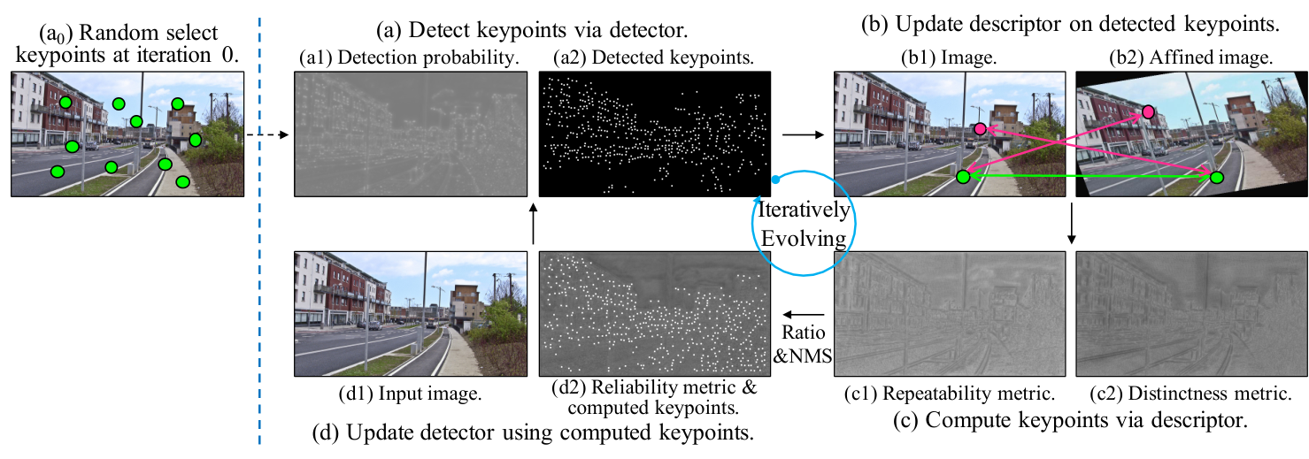
The overview of our framework is shown in Fig. 3, that mainly consists of four steps: (a) compute keypoints probability map using the current detector and subsequently filter the keypoints via non-maximum suppression (NMS) algorithm; (b) update the descriptor branch using the detected keypoints via heightening their descriptors’ repeatability and reliability properties; (c) compute keypoints by figuring out points with reliable (both repeatable and distinct) descriptors; (d) update detector using the newly computed keypoints following detector repeatability and reliability properties. In what follows, we present each step in detail.
4.1 Detect Keypoints using Detector
For an input image , the backbone network extracts feature maps via
| (1) |
The feature maps are subsequently used by the detector branch to estimate the keypoints probability map as
| (2) |
Strong response in each pixel in probability map indicates a potential keypoint, which is further filtered by non-maximum suppression (NMS). We set the suppression radius as 4 pixel in all experiments and set the maximum number of keypoints as during the training process.
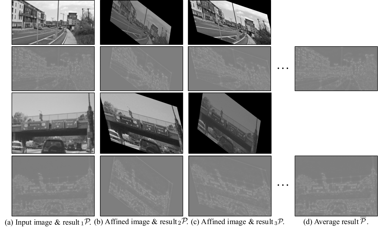
However, the above process is not designed to ensure robust detection of the same keypoints under varying conditions. In other words, the detection process is not optimized to satisfy the detector repeatability property 1.1 and might lead to sub-optimal results. To this end, we adopt a dedicated data augmentation strategy, namely affine adaption superpoint_cvpr18. Specifically, we first apply random affine transformation and color jitter on each input image, and calculate the keypoint probability map. This process is repeated several times, and an average detection result
| (3) |
is computed as the final output, where corresponds to the initial image and the others correspond to the transformed counterparts. Representative examples of the detection process are also demonstrated in Fig. 4. Note that, the affine adaption is only applied during training.
As the detector has not been optimized well at iteration 0, another problem is how to detect keypoints at start. As shown in Fig. 3 (a0), we just randomly select keypoints for each input image. Even so, we show in experiments that the proposed self-evolving framework can converge quickly within just a few iterations.
4.2 Update Keypoint Descriptor
Keypoint descriptor is typically a 2D vector associated with each keypoint, for both re-identifying the same keypoints and distinguishing different keypoints across images. Those descriptor properties are summarized by repeatability property 1.2 and reliability property 2.2 in Sec. 1, that are used as guidelines in our descriptor training process.
To show the details, we note that for each image the keypoint detection process described in Sec. 4.1 provides a set of keypoints . The training process starts by applying random affine transformation and color jitter on both and , leading to
| (4) |
and
| (5) |
By denoting a pair of keypoints, represents a pair of ‘ground-truth’ matched keypoints. According to the descriptor repeatability property 1.2, their descriptors should be close to each other. On the other hand, according to the descriptor reliability property 2.2, should be distinct from others except for its matched keypoint . The representative example of matched and distinct cases are shown in Fig. 3(b) by green and red lines respectively. Inspired by HardNet hardnet_nips17, we use triplet loss along with hard example mining strategy to train the descriptor. Specifically, the loss function is defined as
| (6) |
where is the number of keypoints, denotes the margin parameter, represents the distance, and
| (7) |
| (8) |
| (9) |
The triplet loss function (6) enables the descriptor with both the repeatability property (by (7)) as well as the reliability property (by (8) and (9)).
In addition, as our network shares a common backbone to simultaneously perform keypoint detection and description, the detector branch should also be considered when training the descriptor. To this end, we add a regularization loss term
| (10) |
to maintain the detection results unchanged, where is given by (2) and
| (11) |
, and , are the networks before and after this descriptor training step. The final loss to update the descriptor is
| (12) |
where is the parameter to balance these two losses and is set to be empirically.
4.3 Compute Keypoints via Descriptor
The next step of our self-evolving framework is to compute keypoints from the descriptor maps, that remains a challenging problem in the research community. In our work, we propose to calculate keypoints via evaluating the repeatability property 2.1 and reliability property 2.2 of their corresponding descriptors. Furthermore, as reliability property somehow contains repeatability property, these two properties can be summarized as reliability property and divided into two aspect, namely repeatability and distinctness. Specifically, given the outputs of the descriptor branch and from the original image and its affine transformed counterpart , the descriptor repeatability can be evaluated at each point as:
| (13) |
We point out that the lower is, the more repeatable the descriptor is. In addition, the distinctness of a descriptor can be evaluated as
| (14) |
Similarly, the higher is, the more distinct the descriptor is. As a reliable descriptor should be both repeatable and distinct, we combine the repeatability and distinctness metric into a single metric following the ratio term
| (15) |
Representative examples of computed maps , and are shown in Fig. 5. Someone may find that this ratio term (15) is the same as the ratio in the ratio-test algorithm SIFT_2004_ijcv, that is a well-known method to find keypoints correspondence. This means that the points with higher ratios could be reliably distinguished by subsequently keypoints correspondence finding algorithms. These points, without doubt, should be detected by the detector as much as possible. Therefore, strongly responsive elements on the ratio map are figured out as keypoints via applying NMS algorithm.

Moreover, to ensure high-quality performance, three strategies are applied in the keypoint computing process. Firstly, we note that the ratio map does not cover all points in image , since some elements do not have correspondences in the affine transformed image . Also, to compute keypoints using a single ratio map is not preferred in terms of robustness. To this end, we adopt a data augmentation strategy similar to the affine adaption described in Sec. 4.1. Specifically, we randomly warp the input image via affine transformation, calculate the ratio map, and repeat the same process multiple times to generate an average ratio map
| (16) |
where is corresponding to the th result. An example case of computing the average ratio map is given by Fig. 6.
Secondly, it is important to point out that it is an extremely heavy task to compute . To reduce the computations, we modify as
| (17) |
where contains the local neighbors of point .
Thirdly, the feature maps usually are too coarse for keypoints computing as the descriptor branch consists of a bi-linear up-sampling layer. To this end, we actually use the feature maps and to compute a coarse scale and a fine-scale ratio map respectively and fuse them to obtain the final result.

4.4 Update Keypoint Detector
After the keypoints have been computed via their descriptor reliability, they can be taken as ground-truth to train the detector following the detector reliability property 2.1. We formulate the keypoints detection task as a per-pixel classification task to determine whether the point at each pixel is a keypoint or not. Since the keypoints are very sparse among all the points, we adopt focal loss focal_loss_iccv17 as
| (18) |
where is the computed keypoints.
Besides detector reliability property 2.1, the detector also should be with repeatability property 1.1. To this end, we further adopt affine transformation on the input image and obtain its affined image and detection output . The detector also should rightly detect the keypoints in image , then the detection loss (18) is modified as
| (19) |
where . To further enhance the repeatability property 1.1, we minimize the difference between detection probabilities of corresponding keypoints via the loss
| (20) |
where is the Kullback–Leibler divergence function. To maintain the description results unchanged, we also add a regularization term
| (21) |
where are obtained by the initial network before this detector training step. The final loss to update the detector can be defined as
| (22) |
where empirically in our experiments.
5 Experiments and Comparisons
In this section, we first present the details during training our local feature model, and then compare it with 11 popular methods on homograph estimation, relative pose estimation(stereo), structure-from-motion tasks. At last, we also conduct an ablation experiment to exploit the effectiveness of key training strategies.
5.1 Experimental Details and Comparison Methods
Our local feature model is trained on Microsoft COCO validation dataset cocodataset_eccv14, that consists of realistic images. We repeated the self-evolving iteration times to prevent under-fitting or over-fitting. In each iteration, we train the detector and descriptor epochs in turn and set the initial learning rate as . The learning rate will be multiplied by after the average loss remains un-declining epochs. The whole training process will take 45 hours on a GPU server with two NVIDIA-Tesla-P100 GPUs. To test the inference speed, we deploy our model on a desktop machine with one NVIDIA-GTX-1080Ti GPU to process 10K images with a resolution . Our model can process 301 images per second averagely. We implemented our algorithm based on the PyTorch framework PyTorchNIPS2017.
For affine adaption, we uniformly sample the in-plane rotation, shear, translation, and scale parameters from , respectively. For color jitter, we also uniformly sample the brightness, contrast, saturation, and hue parameters from , respectively.
For comparison methods, we select 6 hand-crafted methods, i.e., ORB orb_iccv11, AKAZE akaze_bmvc13, BRISK brisk_iccv11, SURF surf_eccv06, KAZE kaze_eccv12, and SIFT SIFT_2004_ijcv, that are implemented directly using OpenCV. We also select 5 recently proposed DNN-based methods, i.e., D2-Net d2net_cvpr19, DELF delf_iccv17, LF-Net lfnet_nips18, SuperPoint superpoint_cvpr18, and R2D2 r2d2_nips19. We implement these methods using the codes and models released by the authors. All of these methods can perform keypoints detection and description. The individual detector or descriptor algorithms are not included in the comparison methods since their combinations are various and it is difficult to conduct a fair comparison with methods mentioned above.
Before comparing the performance, we first review the training data (less constraints is better), model size (smaller is better), and dimension of descriptor (lower is better) of each DNN-based method in Tab. 1. On all of these aspects, our method is superior or comparable with other methods.
| Method | Training Data | Model(MB) | Dim. Desc. |
|---|---|---|---|
| D2-Net d2net_cvpr19 | SfM data | 30.5 | 512 float |
| DELF delf_iccv17 | landmarks data | 36.4 | 1024 float |
| LF-Net lfnet_nips18 | SfM data | 31.7 | 256 float |
| SuperPoint superpoint_cvpr18 | rendered&web imgs | 5.2 | 256 float |
| R2D2 r2d2_nips19 | web imgs, SfM data | 2.0 | 128 float |
| SEKD (ours) | web imgs | 2.7 | 128 float |
5.2 Performance on Homography Estimation
Following many previous works, e.g., SIFT_2004_ijcv; superpoint_cvpr18, we also evaluate and compare our method with previous methods via performing the homography estimation task. For benchmark dataset, HPatches hpatches_cvpr17 is adopted as it is the most popular and largest dataset on this task. It includes 117 sequences of images, where each sequence consists of one reference image and five target images. The homography between the reference image and each target image has been carefully calibrated. There are 57 sequences of images only changing in illumination, and 59 sequences of images only changing in viewpoint. We follow most experimental setups and use the homograpy accuracy metric used in superpoint_cvpr18.
To estimate the homography, we use our model and 11 comparison methods to extract the top-500 most confidential keypoints from each input image. The correspondences of keypoints are constructed via nearest matching by descriptors. A cross-check step is further applied to eliminate unstable matches. Then the homography is estimated using the RANSAC algorithm with default parameters via directly calling the function in OpenCV.
As shown in Fig. 7, we plot the homography accuracy curve of each method along with different reprojection error thresholds from 1 through 10. The average homography accuracy (Avg.HA@1:10) is also calculated and presented in Tab. 2. The results of Illumination subset and Viewpoint subset are also presented respectively. The results show that our SEKD model achieves the best overall performance. On the Illumination subset, DELF delf_iccv17 achieves the best result. However, its performance on Viewpoint subset is the worst due to its poor keypoints localization ability. On the Viewpoint subset, our SEKD model outperforms all comparison methods.
| Method | Avg.HA@1:10 on HPatches | mAA on IMC | ||||
|---|---|---|---|---|---|---|
| Mean | ILL. | VIEW. | Mean | Stereo | SfM | |
| ORB orb_iccv11 | 48.96% | 60.28% | 38.03% | 0.064 | 0.032 | 0.097 |
| AKAZE akaze_bmvc13 | 59.22% | 70.63% | 48.20% | 0.190 | 0.079 | 0.302 |
| BRISK brisk_iccv11 | 61.15% | 71.08% | 51.55% | 0.111 | 0.040 | 0.183 |
| SURF surf_eccv06 | 66.77% | 78.94% | 55.01% | 0.238 | 0.149 | 0.328 |
| KAZE kaze_eccv12 | 68.10% | 81.82% | 54.84% | 0.270 | 0.169 | 0.371 |
| SIFT SIFT_2004_ijcv | 74.13% | 84.28% | 64.33% | 0.342 | 0.258 | 0.427 |
| D2-Net d2net_cvpr19 | 30.96% | 47.12% | 15.35% | 0.025 | 0.025 | 0.025 |
| DELF delf_iccv1711 1 On IMC dataset, we reduce the dimension of DELF descriptor from 1024 to 512 using PCA as the benchmark code refuses to take longer descriptors as input. | 50.84% | 98.52% | 4.77% | 0.048 | 0.043 | 0.053 |
| LF-Net lfnet_nips18 | 70.31% | 84.49% | 56.61% | 0.176 | 0.137 | 0.216 |
| SuperPoint superpoint_cvpr18 | 77.65% | 93.15% | 62.67% | 0.395 | 0.231 | 0.559 |
| R2D2 r2d2_nips1922 2 R2D2 adopts image pyramid as input for better performance. For a fair comparison, we only compare the results taking the initial image as input. Actually, with image pyramid as input, the mean results of R2D2 and our method should be updated to 72.81%, 0.442, and, 79.74%, 0.496 on HPatches, IMC respectively. However, this has no influence on the conclusions. | 72.15% | 93.75% | 51.28% | 0.338 | 0.221 | 0.455 |
| SEKD (ours) | 79.98% | 95.29% | 65.18% | 0.430 | 0.307 | 0.553 |
5.3 Performance on Stereo and SfM
The HPathes dataset is a planar dataset and the relation between a pair of images is affine transformation. However, images from unconstrained real environment usually are not satisfy with this constraint. To this end, we resort to the Image Matching Challenge (IMC) dataset imc_2020, that consists of images from 26 scenes and each image is annotated with ground-truth 6-DoF pose. For each scene, IMC collected adequate images to reconstruct the scene and estimate the pose of each image using SfM algorithm. The estimated poses are taken as pseudo ground-truth. Then only a subset of images are selected for evaluation via performing relative pose estimation and struture-from-motion tasks. Via adjusting the error thresholds from 1 to 10 degrees, IMC calculates mean Average Accuracy (mAA) as the metric to compare each method. Please see the website imc_2020 for more details about this dataset.
We adopt the validation set since both the images and ground-truth have been released at the moment. It consists of three scenes, i.e., sacre coeur, st peters square, and reichstag. We extract up to 2K keypoints from each image using each comparison method. Then the keypoints correspondences between each pair of images are constructed via the same matching algorithm, which is the ratio-test in our experiment for float descriptors and nearest-matching for binary descriptors. The mAA metrics are then figured out via evaluating the relative pose estimation and structure-from-motion results. For fair comparison, besides keypoints extraction, all other processes are implemented using the benchmark code released by IMC imc_2020 with the same experimental setups and parameters.
As demonstrated in Tab. 2, our SEKD achieves the best overall performance on the IMC dataset and outperforms the second place method, i.e., SuperPoint superpoint_cvpr18, with a large margin of 0.035. Specifically, on relative pose estimation task, our method outperforms the second place with a large margin of 0.049. On structure-from-motion task, SuperPoint superpoint_cvpr18 slightly outperforms our method with 0.006, however, it achieves unsatisfactory result on relative pose estimation task, that is 0.076 lower than our method. This experiment indicates that, though our SEKD model is trained only using web images with synthetic affine transformations, it has fairly good generalization ability on 3D datasets and problems.
5.4 Effectiveness of Each Training Strategy
To exploit the effectiveness of each key training strategy in our framework, we further conduct an ablation experiment on homography estimation task with HPatches dataset. As shown in Tab. 3, we replace the descriptor repeatability (13) and the descriptor distinctness (14) with the constant value , respectively, then the Avg.HA@1:10 decreases dramatically, that verifies the rationality of our algorithm. We also delete the detector repeatability loss (20) and affine adaption (3)&(16), respectively, the performance also decreases, that verifies that these two strategies can improve the stability of our framework along with the trained model.
| Model | Mean | ILL. | VIEW. |
|---|---|---|---|
| w/o descriptor repeatability (13) | 66.58% | 81.12% | 52.54% |
| w/o descriptor distinctness (14) | 78.03% | 93.68% | 62.91% |
| w/o detector repeatability (20) | 78.03% | 93.92% | 62.67% |
| w/o affine adaption (3)&(16) | 79.05% | 94.24% | 64.37% |
| full method | 79.98% | 95.29% | 65.18% |
6 Discussion and Conclusion
In this paper, we analyze the inherent and interactive properties of local feature detector and descriptor. Guided by the properties, a self-evolving framework is elaborately designed to update the detector and descriptor iteratively using unlabeled images. Extensive experiments verify the effectiveness of our method both on planar and 3D datasets, though our model is trained only using planar data. Moreover, as our framework can work well only using unlabeled data, theoretically, besides natural images, it also can be adopted to discover novel local features from other types of data, e.g., medical images, infrared images, and remote sensing images. We leave these as our future work.
References
- (1) Sameer Agarwal, Yasutaka Furukawa, Noah Snavely, Ian Simon, Brian Curless, Steven M. Seitz, and Richard Szeliski. Building Rome in a Day. Commun. ACM, 54(10):105–112, Oct. 2011.
- (2) Pablo Fernández Alcantarilla, Adrien Bartoli, and Andrew J. Davison. KAZE Features. In ECCV, 2012.
- (3) Vassileios Balntas, Karel Lenc, Andrea Vedaldi, and Krystian Mikolajczyk. HPatches: A Benchmark and Evaluation of Handcrafted and Learned Local Descriptors. In CVPR, 2017.
- (4) Herbert Bay, Tinne Tuytelaars, and Luc Van Gool. SURF: Speeded Up Robust Features. In ECCV, 2006.
- (5) Matthew Brown and David G. Lowe. Automatic Panoramic Image Stitching using Invariant Features. International Journal of Computer Vision, 74(1):59–73, Aug. 2007.
- (6) Liang-Chieh Chen, George Papandreou, Iasonas Kokkinos, Kevin Murphy, and Alan L Yuille. Deeplab: Semantic image segmentation with deep convolutional nets, atrous convolution, and fully connected crfs. IEEE Transactions on Pattern Analysis and Machine Intelligence, 40(4):834–848, 2017.
- (7) Daniel DeTone, Tomasz Malisiewicz, and Andrew Rabinovich. SuperPoint: Self-Supervised Interest Point Detection and Description. In CVPR Workshops, 2018.
- (8) Paolo Di Febbo, Carlo Dal Mutto, Kinh Tieu, and Stefano Mattoccia. KCNN: Extremely-Efficient Hardware Keypoint Detection With a Compact Convolutional Neural Network. In CVPR Workshops, 2018.
- (9) Mihai Dusmanu, Ignacio Rocco, Tomas Pajdla, Marc Pollefeys, Josef Sivic, Akihiko Torii, and Torsten Sattler. D2-Net: A Trainable CNN for Joint Description and Detection of Local Features. In CVPR, 2019.
- (10) Kaiming He, Xiangyu Zhang, Shaoqing Ren, and Jian Sun. Identity Mappings in Deep Residual Networks. In ECCV, 2016.
- (11) Josef Sivic and Andrew Zisserman. Video Google: A Text Retrieval Approach to Object Matching in Videos. In ICCV, 2003.
- (12) Alex Krizhevsky, Ilya Sutskever, and Geoffrey E Hinton. Imagenet classification with deep convolutional neural networks. In NeurIPS, pages 1097–1105, 2012.
- (13) Axel Barroso Laguna, Edgar Riba, Daniel Ponsa, and Krystian Mikolajczyk. Key.Net: Keypoint Detection by Handcrafted and Learned CNN Filters. In ICCV, 2019.
- (14) C. Leng, H. Zhang, B. Li, G. Cai, Z. Pei, and L. He. Local Feature Descriptor for Image Matching: A Survey. IEEE Access, pages 6424–6434, 2019.
- (15) Stefan Leutenegger, Margarita Chli, and Roland Siegwart. BRISK: Binary Robust invariant scalable keypoints. In ICCV, 2011.
- (16) Yunpeng Li, Noah Snavely, Dan Huttenlocher, and Pascal Fua. Worldwide Pose Estimation Using 3D Point Clouds. In ECCV, 2012.
- (17) Tsung-Yi Lin, Priya Goyal, Ross Girshick, Kaiming He, and Piotr Dollár. Focal Loss for Dense Object Detection. In ICCV, 2017.
- (18) Tsung-Yi Lin, Michael Maire, Serge Belongie, James Hays, Pietro Perona, Deva Ramanan, Piotr Dollár, and C Lawrence Zitnick. Microsoft COCO: Common Objects in Context. In ECCV, 2014.
- (19) David G. Lowe. Distinctive Image Features from Scale-Invariant Keypoints. International Journal of Computer Vision, 60(2):91–110, 2004.
- (20) Zixin Luo, Tianwei Shen, Lei Zhou, Jiahui Zhang, Yao Yao, Shiwei Li, Tian Fang, and Long Quan. Contextdesc: Local descriptor augmentation with cross-modality context. CVPR, 2019.
- (21) Zixin Luo, Tianwei Shen, Lei Zhou, Siyu Zhu, Runze Zhang, Yao Yao, Tian Fang, and Long Quan. GeoDesc: Learning local descriptors by integrating geometry constraints. In ECCV, 2018.
- (22) Anastasya Mishchuk, Dmytro Mishkin, Filip Radenovic, and Jiri Matas. Working Hard to Know Your Neighbor’s Margins: Local Descriptor Learning Loss. In NeurIPS, 2017.
- (23) Hyeonwoo Noh, Andre Araujo, Jack Sim, Tobias Weyand, and Bohyung Han. Large-Scale Image Retrieval With Attentive Deep Local Features. In ICCV, 2017.
- (24) Yuki Ono, Eduard Trulls, Pascal Fua, and Kwang Moo Yi. LF-Net: Learning Local Features from Images. In NeurIPS. 2018.
- (25) Adrien Bartoli Pablo Alcantarilla, Jesus Nuevo. Fast Explicit Diffusion for Accelerated Features in Nonlinear Scale Spaces. In BMVC, 2013.
- (26) Adam Paszke, Sam Gross, Soumith Chintala, Gregory Chanan, Edward Yang, Zachary DeVito, Zeming Lin, Alban Desmaison, Luca Antiga, and Adam Lerer. Automatic differentiation in PyTorch. In NeurIPS - Workshop, 2017.
- (27) Shaoqing Ren, Kaiming He, Ross Girshick, and Jian Sun. Faster r-cnn: Towards real-time object detection with region proposal networks. In NeurIPS, pages 91–99, 2015.
- (28) Jerome Revaud, Philippe Weinzaepfel, César De Souza, Noe Pion, Gabriela Csurka, Yohann Cabon, and Martin Humenberger. R2D2: Repeatable and Reliable Detector and Descriptor. In NeurIPS, 2019.
- (29) Ethan Rublee, Vincent Rabaud, Kurt Konolige, and Gary R. Bradski. ORB: An Efficient Alternative to SIFT or SURF. In ICCV, 2011.
- (30) Nikolay Savinov, Akihito Seki, Lubor Ladicky, Torsten Sattler, and Marc Pollefeys. Quad-Networks: Unsupervised Learning to Rank for Interest Point Detection. In CVPR, 2017.
- (31) Edgar Simo-Serra, Eduard Trulls, Luis Ferraz, Iasonas Kokkinos, Pascal Fua, and Francesc Moreno-Noguer. Discriminative Learning of Deep Convolutional Feature Point Descriptors. In ICCV, 2015.
- (32) Yafei Song, Xiaowu Chen, Xiaogang Wang, Yu Zhang, and Jia Li. 6-DOF Image Localization From Massive Geo-Tagged Reference Images. IEEE Transactions on Multimedia, 18(8):1542–1554, 2016.
- (33) Yafei Song, Di Zhu, Jia Li, Yonghong Tian, and Mingyang Li. Learning Local Feature Descriptor with Motion Attribute for Vision-based Localization. In IROS, 2019.
- (34) Yurun Tian, Bin Fan, and Fuchao Wu. L2-Net: Deep Learning of Discriminative Patch Descriptor in Euclidean Space. In CVPR, 2017.
- (35) Eduard Trulls, Yuhe Jin, Kwang Yi, Dmytro Mishkin, Jiri Matas, Anastasiia Mishchuk, and Pascal Fua. Image matching challenge 2020. https://vision.uvic.ca/image-matching-challenge/.
- (36) Yannick Verdie, Kwang Yi, Pascal Fua, and Vincent Lepetit. TILDE: A Temporally Invariant Learned DEtector. In CVPR, 2015.
- (37) Kwang Moo Yi, Eduard Trulls, Vincent Lepetit, and Pascal Fua. LIFT: Learned Invariant Feature Transform. In ECCV, 2016.
- (38) Mingming Zhang, Xingxing Zuo, Yiming Chen, and Mingyang Li. Localization for Ground Robots: On Manifold Representation, Integration, Re-Parameterization, and Optimization. In IROS, 2019.