跳到论文正文
W Papers独立论文阅读器 arXiv:2006.05071 论文正文 计算阅读时间 · 0%
引用这篇论文根据当前论文元数据生成,正式投稿前建议核对。


License: arXiv.org perpetual non-exclusive license
arXiv:2006.05071v1 [cs.SD] 09 Jun 2020

C-SL: Contrastive Sound Localization with Inertial-Acoustic Sensors

Majid Mirbagheri Affiliation: University of Washington Email: mbagheri@uw.edu    Bardia Doosti Affiliation: Indiana University Bloomington Email: bdoosti@indiana.edu
Abstract

Human brain employs perceptual information about the head and eye movements to update the spatial relationship between the individual and the surrounding environment. Based on this cognitive process known as spatial updating, we introduce contrastive sound localization (C-SL) with mobile inertial-acoustic sensor arrays of arbitrary geometry. C-SL uses unlabeled multi-channel audio recordings and inertial measurement unit (IMU) readings collected during free rotational movements of the array to learn mappings from acoustical measurements to an array-centered direction-of-arrival (DOA) in a self-supervised manner. Contrary to conventional DOA estimation methods that require the knowledge of either the array geometry or source locations in the calibration stage, C-SL is agnostic to both, and can be trained on data collected in minimally constrained settings. To achieve this capability, our proposed method utilizes a customized contrastive loss measuring the spatial contrast between source locations predicted for disjoint segments of the input to jointly update estimated DOAs and the acoustic-spatial mapping in linear time. We provide quantitative and qualitative evaluations of C-SL comparing its performance with baseline DOA estimation methods in a wide range of conditions. We believe the relaxed calibration process offered by C-SL paves the way toward truly personalized augmented hearing applications.

1 Introduction

Humans localize sounds by comparing inputs across the two ears, resulting in a head-centered representation of sound-source location [1]. When the head moves, brain combines inertial information about head movement with the head-centered estimate to correctly update the world-centered sound-source location in a cognitive process known as auditory spatial updating [2, 3]. Existing methods for sound localization with microphone arrays differ from human auditory system in two major aspects: (i) unlike humans who adapt to changes in auditory localization cues without supervision [4], in order to operate, these algorithms rely on either specific array geometries or access to sample sounds with known spatial information. (ii) these methods do not account for array movements as they are mostly designed for static applications. With the advent of augmented reality (AR) technologies embodied in mobile devices such as smart glasses and headphones, addressing these gaps can extend versatility of these algorithms to more applications in this domain.

Calibration of the arrays in conventional source localization methods involves measuring array responses to signals coming from known directions when they cannot be analytically determined as a function of the array geometry. Once the array is calibrated, these methods use stored responses as some form of lookup table. Popular methods in this category consist of those based on steered response power (SRP) [5] and subspace approaches such as multiple signal classification (MUSIC) [6]. The grid search involved in these methods is, however, usually of considerable computational cost, while the performance is restricted by the grid resolution.

In an effort to overcome these issues, more recently supervised learning algorithms using deep neural networks (DNN) have gained significant attention in the field [7, 8, 9, 10, 11, 12]. Given acoustic measurements with known spatial labels, in the form of a single direction or spherical intensity field representations, DNN-based methods solve a nonlinear regression problem to predict labels from measurements via an iterative gradient-based optimization algorithm. A common problem of learning-based methods is their sensitivity to mismatches between distributions of data used for training and test. This issues can be specifically more severe for mobile arrays with microphones that are fit in the ear or installed on head-mounted or hand-held devices. The directional pattern of such arrays depends on not only relative positioning of the microphones but also the unique anatomical geometry of the users’ head/ear, the device fit, or how the device is handled by the user. On one hand, augmenting training sets with all such variabilities is in general an infeasible task, and this eliminates the possibility of calibrating the array prior to deployment. On the other hand, collection of acoustic data with clean spatial labels cannot currently take place on a per user basis as it requires elaborate lab setups or computationally-expensive simulations.

Contrastive learning is an emerging paradigm proposed to overcome data limitations of supervised methods through self-supervision namely automatic labeling of data by comparing different views of it across time, space, or sensor modalities [13, 14, 15]. This paradigm has been successfully used for visual object detection [16, 17], and audio-visual source localization [18, 19, 20, 21]. Studies in neuroscience suggest that human brain utilizes predictive coding, a special form of self-supervision, to encode sound attributes [22]. Spatial updating process in brain also by nature uses a contrastive measure based on spatial displacement of the head to update head-centered sound source location as the individual moves [2, 3]. Inertial information involved in calculation of head attitude and motion is provided by vestibular organs in the inner ear. While this process has been mostly investigated in the context of localization inference, a contrastive learning framework for sound localization based on spatial updating that imitates plasticity in spatial auditory processing is yet to be desired. Such a framework will bridge the gaps between traditional DOA estimation methods and human spatial auditory processing. In applications, inertial information has been previously utilized to increase robustness of visual odometry [23, 24] and simultaneous localization and mapping (SLAM) systems [25].

Contributions In this paper, we propose to the best of our knowledge the first contrastive learning framework for sound localization with inertial-acoustic sensors based on cognitive process of auditory spatial updating. Our algorithm, named C-SL, is able to localize both narrowband and wideband sources, and in contrast to existing DNN and grid search-based methods, is agnostic to the array geometry and the knowledge of source locations in the calibration process. The only assumption we make is that during training there is only one far-field source present, and that the location of this source is approximately piece-wise constant in a reference coordinate frame which we refer to as world-frame in the rest of the paper. To train our model, we use a customized loss that leverages this assumption and minimizes spatial contrast between predictions for consecutive segments of input in the calibration stage. In the next section, we describe the data model followed by how the contrastive loss is computed, and the model architecture.

2 Self-Supervised Learning with Sub-Contrastive Loss

2.1 Data Model

Assuming a single far-field sound wave impinging on a microphone array, the output of the microphone with the index m∈{1,…,M}m\in\{1,\dots,M\} is given in the short-time Fourier transform (STFT) domain by:

Yk,nm=Hkm​(rns)​Sk,n+Vk,nmY^{m}_{k,n}=H^{m}_{k}(r^{s}_{n})S_{k,n}+V^{m}_{k,n} (1)

where Sk,nS_{k,n} is the source signal, Hkm​(rns)H^{m}_{k}(r^{s}_{n}) is the acoustic transfer functions (ATF) of the source at location rnsr^{s}_{n} with respect to mm-th microphone, Vk,nmV^{m}_{k,n} models noise and reverberation, and kk and nn are the frequency and time frame indices, respectively. Since we are interested about far-field localization, we denote the source location as a 3-D vector on the unit sphere, rs∈𝕊2r^{s}\in\mathbb{S}^{2}. With this definition, the locations will be the same for all microphones, hence referred to as sensor-frame direction. Throughout the paper, bold symbols represent MM-dimensional vectorized version of quantities related to the microphone array, ⟨⋅,⋅⟩\langle\cdot{,}\cdot\rangle is the inner product, ‖x‖\left\lVert x\right\rVert denotes ℓ2\ell_{2} norm of a vector, and x^=x‖x‖\hat{x}=\frac{x}{\left\lVert x\right\rVert} for all vectors x≠0x\neq 0.

During train data collection the array is rotated in all directions to densely sample acoustic measurements along arbitrary trajectories on 𝕊2\mathbb{S}^{2}. With a 9-DOF inertial measurement unit (IMU) attached to the array, orientations of the array with respect to the earth (world) frame, represented by quaternions or Euler angles, can be calculated from raw IMU readings [26]. Given the correspondence between orientations and rotation matrices in 3-D space [27], we assume that for any given time frame we know the corresponding rotation matrix Rn∈SO​(3)R_{n}\in\mbox{SO}(3) with which we can transform any direction in the sensor coordinate to the world frame coordinate by:

rnw=Rn​rnsr^{w}_{n}=R_{n}r^{s}_{n} (2)

Spatial Constancy: Considering that rwr^{w} changes at a slow rate (in contrast to rsr^{s}), we assume it to be (approximately) constant over time intervals, denoted by {Ii}i=1Ni\{I_{i}\}_{i=1}^{N_{i}}, with Ii={n}ni≤n<ni+1I_{i}=\{n\}_{n_{i}\leq n<n_{i+1}}, 1=n1<n2<⋯<nNi+1=Ns1=n_{1}<n_{2}<\dots<n_{N_{i}+1}=N_{s}, and NsN_{s}, NiN_{i} representing the total number of samples and intervals. For the sake of generality, we do not assume any special relationship between source locations across different intervals.

2.2 Sub-Contrastive Loss

Given the observations {(𝒀k,n,Rn)}\{(\bm{Y}_{k,n},R_{n})\}, and {Ii}\{I_{i}\}, we seek an acoustic-spatial function fθ:ℂM×(0,1]→𝕊2f_{\theta}\colon\mathbb{C}^{M}\times\left(0,1\right]\rightarrow\mathbb{S}^{2}, parameterized by θ\theta, that maps MM-dimensional complex-valued acoustic measurements at each time-frequency bin, 𝒀k,n\bm{Y}_{k,n}, and their associated normalized frequency, k~=k/kmax\tilde{k}=k/k_{\max}, to a single direction in the sensor frame.

We can find the optimum values of θ\theta in a self-supervised manner by leveraging the spatial constancy assumption i.e. maximizing pairwise similarity between world-frame directions predicted for all the time-frequency bins within intervals {Ii}\{I_{i}\} with a contrastive loss expressed by:

ℒcont​(θ)=∑i=1Ni∑m,n∈Iik,k′‖r~k,mw−r~k′,nw‖2\displaystyle\mathcal{L}_{\mathrm{cont}}(\theta)=\sum\limits_{i=1}^{N_{i}}\ \sum\limits_{\begin{subarray}{c}m,n\in I_{i}\\ k,k^{\prime}\end{subarray}}\ \left\lVert\tilde{r}^{w}_{k,m}-\tilde{r}^{w}_{k^{\prime},n}\right\rVert^{2} (3)

where r~k,nw=Rn​fθ​(𝒀k,n,k~).(4)\tilde{r}^{w}_{k,n}=R_{n}f_{\theta}(\bm{Y}_{k,n},\tilde{k}).\hfill(4)

This loss function uniquely determines the mapping ff up to an inversion of the sign, when the mapping is bijective and the loss takes its minimum value of 0 over all possible pairs of observations (for a proof see the Appendix). In a conventional contrastive learning framework, the loss function not only encourages outputs to be close for similar (positive) examples, but also forces them away from one another for distant (negative) ones. The loss defined in (3) accomplishes this in a soft manner by constraining the spatial contrast between sensor-frame directions predicted for different pairs based on the measured change in the orientation of the of the array.

Pairwise similarity imposes a fairly strong constraint on predicted directions causing the training to fail entirely when some of the bins are dominated by spurious directions caused by reverberation, or ambient noise. In order to manage such situations, we propose a simple cost function, termed sub-contrastive loss, that enforces a weaker similarity constraint over the entire set of interval bins. Furthermore, to handle uncertainty, we expand the range of fθf_{\theta} to ℝ3\mathbb{R}^{3} so that the mapping predicts an additional positive-valued weight, encoded in the norm of the output, representing the confidence of the predicted direction for the bin.

Figure 1 shows how sub-contrastive loss is computed from world-frame directions predicted for different time-frequency bins. We first break each interval IiI_{i} into two disjoint sub-intervals denoted by {(Ii,1,Ii,2)}\{(I_{i,1},I_{i,2})\}. Break points are chosen randomly so that the ratio of bins in the two segments satisfies c1≤|Ii,1||Ii,2|≤c2c_{1}\leq\frac{\lvert I_{i,1}\rvert}{\lvert I_{i,2}\rvert}\leq c_{2} with c1c_{1} and c2c_{2} arbitrarily set to 0.2 and 0.8.

We then pool the world-frame directions predicted by (4) over all time-frequency bins in each sub-interval by finding their centroid on 𝕊2\mathbb{S}^{2} formulated as:

r¯i,lw=argmind∈𝕊2∑n∈Ii,l,k‖d−r~k,nw‖2=(∑n∈Ii,l,kr~k,nw)^,l=1,2\bar{r}_{i,l}^{w}=\argmin_{d\in\mathbb{S}^{2}}\sum\limits_{n\in I_{i,l},k}\left\lVert d-\tilde{r}^{w}_{k,n}\right\rVert^{2}=\mathchoice{\widehat{\hbox{$\displaystyle\left(\sum\limits_{n\in I_{i,l},k}\tilde{r}^{w}_{k,n}\right)$}}}{\widehat{\hbox{$\textstyle\left(\sum\limits_{n\in I_{i,l},k}\tilde{r}^{w}_{k,n}\right)$}}}{\widehat{\hbox{$\scriptstyle\left(\sum\limits_{n\in I_{i,l},k}\tilde{r}^{w}_{k,n}\right)$}}}{\widehat{\hbox{$\scriptscriptstyle\left(\sum\limits_{n\in I_{i,l},k}\tilde{r}^{w}_{k,n}\right)$}}},\quad l=1,2 (5)

Note that by preserving the norms during sensor-to-world transformation, we favor the high-confidence predictions over the rest in the pooling stage. Finally, the sub-contrastive loss measures the distance between the two centroids computed for the sub-interval pairs as followed:

ℒsub-cont​(θ)=∑i=1Ni‖r¯i,1w−r¯i,2w‖2\mathcal{L}_{\text{sub-cont}}(\theta)=\sum\limits_{i=1}^{N_{i}}\ \left\lVert\bar{r}_{i,1}^{w}-\bar{r}_{i,2}^{w}\right\rVert^{2} (6)

A minimum value of 00 for the sub-contrastive loss is only a necessary condition to meet the pairwise similarity constraint. Thus the this loss can be seen as a weaker form of the contrastive one. It should be noted that using random subsets of bins from intervals to compute the centroids results in same degenerate sensor predictions. The time-based segmentation described above avoids this situation by considering only subsets with likely most different array orientations and making sure their world frame centroids are matching. Randomizing break points across training epochs improves stochasticity and consequently generalizability of the model.

Similar to contrastive one, the sub-contrastive loss is invariant to reflection of predicted sensor frame directions with respect to the origin. This sign ambiguity in the predictions can be easily resolved in many cases via a postprocessing stage in which fθf_{\theta} is negated based on additional criteria. For instance, when simple knowledge about relative position of microphones such as “mic A coordinate in the sensor frame has a larger value on the xx-axis than mic B” is available, a comparison of intensities or delays of sounds received at the two microphones can determine if the predicted directions should be reflected or not. Alternatively, orientation of the array at the beginning of data collection can be set with respect to the source in a way that a general condition such as ⟨rn=0s,i^⟩>0\langle r^{s}_{n=0},\bm{\hat{\textbf{i}}}\rangle>0 is enforced and later used to disambiguate the mapping.

The centroids computed in (5) can be interpreted as denoised approximation of predicted world-frame directions. At the time of training, we need two versions of this estimate for each interval to make contrastive learning possible. However at the time of inference, there is no such need, and centroids can be computed directly over all time-frequency bins within the each interval providing that they all belong to the same source. In multi-source conditions, world-frame predictions for different bins appear in clusters representing different sources to which they belong. As we will see in Section 3, in such situations, we can run a clustering algorithm on these predictions in the same vein as [28], and use associated cluster centers as denoised approximation of world-frame directions for each bin. Regardless of number of sources, denoised sensor-frame directions are computed by transforming the world-frame centroids back into the sensor frame for each time-frequency bin.

In contrast to quadratic time of contrastive loss, computation of the sub-contrastive loss only takes linear time with respect to the number of time-frequency bins resulting in a very efficient training of the model by C-SL.

2.3 Model Architecture

We design fθf_{\theta} as a multi-layer perceptron (MLP), agnostic to the underlying spatial configuration of the array (as opposed to a convnet, for example). The MLP we use consists of three hidden layers with 1024, 512, and 256 units. Each hidden layer is followed by a (parameter-free) weight normalization layer [29] and a standard ReLU non-linearity. The third hidden layer provides the input to a linear prediction layer of size three.

It should be noted that while fθf_{\theta} could be optimized separately for each frequency, we opt for a single mapping conditioned on frequency in the view of the fact that the array spectral profile is inherently low dimensional.

3 Experiments

Algorithm 1 C-SL Training 1:  θ\theta ←\leftarrow Initialize model parameters. 2:  while not converged do 3:   B⊂{1,…,Ni}B\subset\{1,\dots,N_{i}\} ←\leftarrow random mini-batch of interval indices 4:   𝒀k,n\bm{Y}_{k,n}, RnR_{n}, ←\leftarrow data at intervals {Ii}i∈B\{I_{i}\}_{i\in B} 5:   {(Ii,1,Ii,2)}←\{(I_{i,1},I_{i,2})\}\leftarrow sub-intervals with random break points 6:   r~k,ns←fθ​(𝒀k,n,k~)\tilde{r}^{s}_{k,n}\leftarrow f_{\theta}(\bm{Y}_{k,n},\tilde{k}) 7:   r~k,nw←Rn​r~k,ns\tilde{r}^{w}_{k,n}\leftarrow R_{n}\tilde{r}^{s}_{k,n} 8:   r¯i,lw←(∑n∈Ii,l,kr~k,nw)^i∈B,l=1,2\bar{r}_{i,l}^{w}\leftarrow\mathchoice{\widehat{\hbox{$\displaystyle\left(\sum\limits_{n\in I_{i,l},k}\tilde{r}^{w}_{k,n}\right)$}}}{\widehat{\hbox{$\textstyle\left(\sum\limits_{n\in I_{i,l},k}\tilde{r}^{w}_{k,n}\right)$}}}{\widehat{\hbox{$\scriptstyle\left(\sum\limits_{n\in I_{i,l},k}\tilde{r}^{w}_{k,n}\right)$}}}{\widehat{\hbox{$\scriptscriptstyle\left(\sum\limits_{n\in I_{i,l},k}\tilde{r}^{w}_{k,n}\right)$}}}\quad i\in B,\,l=1,2 9:   ℒsub-cont←∑i∈S‖r¯i,1w−r¯i,2w‖2\mathcal{L}_{\text{sub-cont}}\leftarrow\sum\limits_{i\in S}\ \left\lVert\bar{r}_{i,1}^{w}-\bar{r}_{i,2}^{w}\right\rVert^{2} 10:   θ←Adam​(▽θ,ℒsub-cont,θ)\theta\leftarrow\text{A}\textsc{dam}(\triangledown_{\theta},\mathcal{L}_{\text{sub-cont}},\theta) 11:  end while 12:  if reflection condition satisfied then 13:   fθ←−fθf_{\theta}\leftarrow-f_{\theta} 14:  end if [Uncaptioned image] Figure 1: Overview of the proposed framework for Contrastive Sound Localization (C-SL). Sensor-frame predictions are transformed into the world frame (S→WS\rightarrow W) by the help of inertial information provided by the IMU. During training, sub-contrastive loss measures distance between world-frame predictions aggregated over time-frequency bins within sub-intervals of data.

3.1 Dataset

In order to evaluate the proposed C-SL, we synthesize a dataset consisting of hybrid acoustic-inertial data in the same vein as most DNN-based methods which need large amount of data [7, 8, 9, 11]. Our dataset consists of multiple recording sessions. Each session simulates acoustic-inertial data from one interval described in section 2.1. We simulate measurements in a 4×4×4 m4\times 4\times 4\text{\,}\mathrm{m} room with point sources randomly placed 1 m1\text{\,}\mathrm{m} away from the room center. Source locations remain consistent within a particular session, but vary from session to session. Without loss of generality, we use an array with cubical configuration with 8 omni-directional microphones positioned at the corners of a cube with an edge length of 5 cm5\text{\,}\mathrm{c}\mathrm{m} and center of mass always at the room center. For the array motion, we consider rotations at a constant angular velocity of magnitude π2 rad\frac{\pi}{2}\text{\,}\mathrm{rad} and fixed but random axes for each session. Orientation of the array at the beginning of each session is set to a unit quaternion randomly chosen from 𝕊3\mathbb{S}^{3}. Translational motion was not considered in our experiments in order to avoid violating the far-filed assumption. We calculated room impulse responses in five different reverbrant room conditions, four with fixed reverberation times, and one with mixed reverberation times. In all conditions, we used a GPU-based geometrical acoustics simulator, gpuRIR [30] to model sound propagation and reverberation based on the rectangular room image-source model [31]. In the first four conditions, we set the value of broadband reverberation time of the room T60T_{60} respectively to 0 (anechoic), 250, 500, and 750 ms750\text{\,}\mathrm{m}\mathrm{s}. For the last condition, we randomly sampled T60T_{60} values from the range 0 ms-750 ms0\text{\,}\mathrm{m}\mathrm{s}750\text{\,}\mathrm{m}\mathrm{s} for each session. We refer to these five conditions as CanechoicC_{\text{anechoic}}, C250C_{250}, C500C_{500}, C750C_{750}, and CmixedC_{\text{mixed}}. To generate one session with a single source in each of these conditions, one dry speech recording from the TIMIT corpus [32] with an average length of approximately 3 s3\text{\,}\mathrm{s} was convolved with the simulated room impulse responses. We split 6300 utterances in the corpus into three subsets of size 5012, 638, and 638 respectively for train, test and validation. All utterances in the three splits were then spatialized each resulting in one session in the corresponding split. All recordings, sampled at 16 kHz16\text{\,}\mathrm{k}\mathrm{H}\mathrm{z}, were transformed into the STFT domain using frames of length 25 ms25\text{\,}\mathrm{m}\mathrm{s}, hop length 10 ms10\text{\,}\mathrm{m}\mathrm{s} and a hanning window. Rotation matrices associated with time frames were calculated based on angular velocity and initial orientation of the array chosen for the session and the timestamp of the frames.

The input features to the network are 17×117\times 1 vectors computed for each time-frequency bin, consisting of real and imaginary parts of the array STFT coefficients concatenated and normalized to a unit-norm 16×116\times 1 vector and an additional feature representing normalized frequency of the bin. The normalization of acoustic features instructs the model to disregard content and distance-related variations of intensity across time and frequency.

In order to save memory and also satisfy the far-filed assumption, during training from each session we only picked bins in the frequency range 340 Hz to 8000 Hz340\text{\,}\mathrm{H}\mathrm{z}8000\text{\,}\mathrm{H}\mathrm{z} whose original STFT magnitudes were greater than some ratio (arbitrarily set to -40 dB) of the maximum magnitude over all the bins with the same frequency.

3.2 Training and Metric

We optimized parameters of the model iteratively on selected mini-batches of simulated sessions from CmixedC_{\text{mixed}} dataset. We used the Adam optimizer [33] with β1=0.9\beta_{1}=0.9 and β2=0.999\beta_{2}=0.999, a learning rate of 1×10−051\text{\times}{10}^{-05}, and batch size of 8. All models were trained with 2 GPUs for 300 epochs. The procedural training details are summarized in Algorithm 1.

We used the angle (in degrees) between estimated sensor-frame directions and their ground truth values used in the simulation, formulated by σ⁡(r¯s,rs)=180/π⋅cos−1⁡(⟨r¯s,rs⟩)\sigma(\bar{r}^{s},r^{s})=180/\pi\cdot\cos^{-1}(\langle\bar{r}^{s},r^{s}\rangle), as the DOA estimation error metric in our evaluations. In particular for C-SL, r¯s\bar{r}^{s} refers to the final denoised sensor-frame estimates.

Table 1: Comparison of DOA estimation errors (in degree) in single-source condition evaluated for different reverberations times, and window lengths LwinL_{\text{win}}.
Method Lwin​(s)L_{\text{win}}($\mathrm{s}$) CAnechoicC_{\text{Anechoic}} C250C_{250} C500C_{500} C750C_{750}
SRP-PHAT [5] 0.05 1.17​±0.011.17{\color[rgb]{0.5,0.5,0.5}\mathchoice{\raisebox{-0.64655pt}{\resizebox{1610148}{327680}{\hbox{\raisebox{0.83333pt}{$\displaystyle\pm 0.01$}}}}}{\raisebox{-0.64655pt}{\resizebox{1610148}{327680}{\hbox{\raisebox{0.83333pt}{$\textstyle\pm 0.01$}}}}}{\raisebox{-0.92365pt}{\resizebox{1930967}{327680}{\hbox{\raisebox{0.83334pt}{$\scriptstyle\pm 0.01$}}}}}{\raisebox{-1.25002pt}{\resizebox{2334712}{327680}{\hbox{\raisebox{0.83336pt}{$\scriptscriptstyle\pm 0.01$}}}}}} 3.28​±0.123.28{\color[rgb]{0.5,0.5,0.5}\mathchoice{\raisebox{-0.64655pt}{\resizebox{1610148}{327680}{\hbox{\raisebox{0.83333pt}{$\displaystyle\pm 0.12$}}}}}{\raisebox{-0.64655pt}{\resizebox{1610148}{327680}{\hbox{\raisebox{0.83333pt}{$\textstyle\pm 0.12$}}}}}{\raisebox{-0.92365pt}{\resizebox{1930967}{327680}{\hbox{\raisebox{0.83334pt}{$\scriptstyle\pm 0.12$}}}}}{\raisebox{-1.25002pt}{\resizebox{2334712}{327680}{\hbox{\raisebox{0.83336pt}{$\scriptscriptstyle\pm 0.12$}}}}}} 11.35​±0.3011.35{\color[rgb]{0.5,0.5,0.5}\mathchoice{\raisebox{-0.64655pt}{\resizebox{1610148}{327680}{\hbox{\raisebox{0.83333pt}{$\displaystyle\pm 0.30$}}}}}{\raisebox{-0.64655pt}{\resizebox{1610148}{327680}{\hbox{\raisebox{0.83333pt}{$\textstyle\pm 0.30$}}}}}{\raisebox{-0.92365pt}{\resizebox{1930967}{327680}{\hbox{\raisebox{0.83334pt}{$\scriptstyle\pm 0.30$}}}}}{\raisebox{-1.25002pt}{\resizebox{2334712}{327680}{\hbox{\raisebox{0.83336pt}{$\scriptscriptstyle\pm 0.30$}}}}}} 16.96​±0.3916.96{\color[rgb]{0.5,0.5,0.5}\mathchoice{\raisebox{-0.64655pt}{\resizebox{1610148}{327680}{\hbox{\raisebox{0.83333pt}{$\displaystyle\pm 0.39$}}}}}{\raisebox{-0.64655pt}{\resizebox{1610148}{327680}{\hbox{\raisebox{0.83333pt}{$\textstyle\pm 0.39$}}}}}{\raisebox{-0.92365pt}{\resizebox{1930967}{327680}{\hbox{\raisebox{0.83334pt}{$\scriptstyle\pm 0.39$}}}}}{\raisebox{-1.25002pt}{\resizebox{2334712}{327680}{\hbox{\raisebox{0.83336pt}{$\scriptscriptstyle\pm 0.39$}}}}}}
0.2 1.16​±0.011.16{\color[rgb]{0.5,0.5,0.5}\mathchoice{\raisebox{-0.64655pt}{\resizebox{1610148}{327680}{\hbox{\raisebox{0.83333pt}{$\displaystyle\pm 0.01$}}}}}{\raisebox{-0.64655pt}{\resizebox{1610148}{327680}{\hbox{\raisebox{0.83333pt}{$\textstyle\pm 0.01$}}}}}{\raisebox{-0.92365pt}{\resizebox{1930967}{327680}{\hbox{\raisebox{0.83334pt}{$\scriptstyle\pm 0.01$}}}}}{\raisebox{-1.25002pt}{\resizebox{2334712}{327680}{\hbox{\raisebox{0.83336pt}{$\scriptscriptstyle\pm 0.01$}}}}}} 1.96​±0.061.96{\color[rgb]{0.5,0.5,0.5}\mathchoice{\raisebox{-0.64655pt}{\resizebox{1610148}{327680}{\hbox{\raisebox{0.83333pt}{$\displaystyle\pm 0.06$}}}}}{\raisebox{-0.64655pt}{\resizebox{1610148}{327680}{\hbox{\raisebox{0.83333pt}{$\textstyle\pm 0.06$}}}}}{\raisebox{-0.92365pt}{\resizebox{1930967}{327680}{\hbox{\raisebox{0.83334pt}{$\scriptstyle\pm 0.06$}}}}}{\raisebox{-1.25002pt}{\resizebox{2334712}{327680}{\hbox{\raisebox{0.83336pt}{$\scriptscriptstyle\pm 0.06$}}}}}} 4.16​±0.194.16{\color[rgb]{0.5,0.5,0.5}\mathchoice{\raisebox{-0.64655pt}{\resizebox{1610148}{327680}{\hbox{\raisebox{0.83333pt}{$\displaystyle\pm 0.19$}}}}}{\raisebox{-0.64655pt}{\resizebox{1610148}{327680}{\hbox{\raisebox{0.83333pt}{$\textstyle\pm 0.19$}}}}}{\raisebox{-0.92365pt}{\resizebox{1930967}{327680}{\hbox{\raisebox{0.83334pt}{$\scriptstyle\pm 0.19$}}}}}{\raisebox{-1.25002pt}{\resizebox{2334712}{327680}{\hbox{\raisebox{0.83336pt}{$\scriptscriptstyle\pm 0.19$}}}}}} 6.67​±0.356.67{\color[rgb]{0.5,0.5,0.5}\mathchoice{\raisebox{-0.64655pt}{\resizebox{1610148}{327680}{\hbox{\raisebox{0.83333pt}{$\displaystyle\pm 0.35$}}}}}{\raisebox{-0.64655pt}{\resizebox{1610148}{327680}{\hbox{\raisebox{0.83333pt}{$\textstyle\pm 0.35$}}}}}{\raisebox{-0.92365pt}{\resizebox{1930967}{327680}{\hbox{\raisebox{0.83334pt}{$\scriptstyle\pm 0.35$}}}}}{\raisebox{-1.25002pt}{\resizebox{2334712}{327680}{\hbox{\raisebox{0.83336pt}{$\scriptscriptstyle\pm 0.35$}}}}}}
0.5 1.27​±0.031.27{\color[rgb]{0.5,0.5,0.5}\mathchoice{\raisebox{-0.64655pt}{\resizebox{1610148}{327680}{\hbox{\raisebox{0.83333pt}{$\displaystyle\pm 0.03$}}}}}{\raisebox{-0.64655pt}{\resizebox{1610148}{327680}{\hbox{\raisebox{0.83333pt}{$\textstyle\pm 0.03$}}}}}{\raisebox{-0.92365pt}{\resizebox{1930967}{327680}{\hbox{\raisebox{0.83334pt}{$\scriptstyle\pm 0.03$}}}}}{\raisebox{-1.25002pt}{\resizebox{2334712}{327680}{\hbox{\raisebox{0.83336pt}{$\scriptscriptstyle\pm 0.03$}}}}}} 2.41​±0.112.41{\color[rgb]{0.5,0.5,0.5}\mathchoice{\raisebox{-0.64655pt}{\resizebox{1610148}{327680}{\hbox{\raisebox{0.83333pt}{$\displaystyle\pm 0.11$}}}}}{\raisebox{-0.64655pt}{\resizebox{1610148}{327680}{\hbox{\raisebox{0.83333pt}{$\textstyle\pm 0.11$}}}}}{\raisebox{-0.92365pt}{\resizebox{1930967}{327680}{\hbox{\raisebox{0.83334pt}{$\scriptstyle\pm 0.11$}}}}}{\raisebox{-1.25002pt}{\resizebox{2334712}{327680}{\hbox{\raisebox{0.83336pt}{$\scriptscriptstyle\pm 0.11$}}}}}} 4.59​±0.274.59{\color[rgb]{0.5,0.5,0.5}\mathchoice{\raisebox{-0.64655pt}{\resizebox{1610148}{327680}{\hbox{\raisebox{0.83333pt}{$\displaystyle\pm 0.27$}}}}}{\raisebox{-0.64655pt}{\resizebox{1610148}{327680}{\hbox{\raisebox{0.83333pt}{$\textstyle\pm 0.27$}}}}}{\raisebox{-0.92365pt}{\resizebox{1930967}{327680}{\hbox{\raisebox{0.83334pt}{$\scriptstyle\pm 0.27$}}}}}{\raisebox{-1.25002pt}{\resizebox{2334712}{327680}{\hbox{\raisebox{0.83336pt}{$\scriptscriptstyle\pm 0.27$}}}}}} 6.63​±0.436.63{\color[rgb]{0.5,0.5,0.5}\mathchoice{\raisebox{-0.64655pt}{\resizebox{1610148}{327680}{\hbox{\raisebox{0.83333pt}{$\displaystyle\pm 0.43$}}}}}{\raisebox{-0.64655pt}{\resizebox{1610148}{327680}{\hbox{\raisebox{0.83333pt}{$\textstyle\pm 0.43$}}}}}{\raisebox{-0.92365pt}{\resizebox{1930967}{327680}{\hbox{\raisebox{0.83334pt}{$\scriptstyle\pm 0.43$}}}}}{\raisebox{-1.25002pt}{\resizebox{2334712}{327680}{\hbox{\raisebox{0.83336pt}{$\scriptscriptstyle\pm 0.43$}}}}}}
1.0 2.30​±0.092.30{\color[rgb]{0.5,0.5,0.5}\mathchoice{\raisebox{-0.64655pt}{\resizebox{1610148}{327680}{\hbox{\raisebox{0.83333pt}{$\displaystyle\pm 0.09$}}}}}{\raisebox{-0.64655pt}{\resizebox{1610148}{327680}{\hbox{\raisebox{0.83333pt}{$\textstyle\pm 0.09$}}}}}{\raisebox{-0.92365pt}{\resizebox{1930967}{327680}{\hbox{\raisebox{0.83334pt}{$\scriptstyle\pm 0.09$}}}}}{\raisebox{-1.25002pt}{\resizebox{2334712}{327680}{\hbox{\raisebox{0.83336pt}{$\scriptscriptstyle\pm 0.09$}}}}}} 3.80​±0.163.80{\color[rgb]{0.5,0.5,0.5}\mathchoice{\raisebox{-0.64655pt}{\resizebox{1610148}{327680}{\hbox{\raisebox{0.83333pt}{$\displaystyle\pm 0.16$}}}}}{\raisebox{-0.64655pt}{\resizebox{1610148}{327680}{\hbox{\raisebox{0.83333pt}{$\textstyle\pm 0.16$}}}}}{\raisebox{-0.92365pt}{\resizebox{1930967}{327680}{\hbox{\raisebox{0.83334pt}{$\scriptstyle\pm 0.16$}}}}}{\raisebox{-1.25002pt}{\resizebox{2334712}{327680}{\hbox{\raisebox{0.83336pt}{$\scriptscriptstyle\pm 0.16$}}}}}} 7.15​±0.447.15{\color[rgb]{0.5,0.5,0.5}\mathchoice{\raisebox{-0.64655pt}{\resizebox{1610148}{327680}{\hbox{\raisebox{0.83333pt}{$\displaystyle\pm 0.44$}}}}}{\raisebox{-0.64655pt}{\resizebox{1610148}{327680}{\hbox{\raisebox{0.83333pt}{$\textstyle\pm 0.44$}}}}}{\raisebox{-0.92365pt}{\resizebox{1930967}{327680}{\hbox{\raisebox{0.83334pt}{$\scriptstyle\pm 0.44$}}}}}{\raisebox{-1.25002pt}{\resizebox{2334712}{327680}{\hbox{\raisebox{0.83336pt}{$\scriptscriptstyle\pm 0.44$}}}}}} 9.11​±0.609.11{\color[rgb]{0.5,0.5,0.5}\mathchoice{\raisebox{-0.64655pt}{\resizebox{1610148}{327680}{\hbox{\raisebox{0.83333pt}{$\displaystyle\pm 0.60$}}}}}{\raisebox{-0.64655pt}{\resizebox{1610148}{327680}{\hbox{\raisebox{0.83333pt}{$\textstyle\pm 0.60$}}}}}{\raisebox{-0.92365pt}{\resizebox{1930967}{327680}{\hbox{\raisebox{0.83334pt}{$\scriptstyle\pm 0.60$}}}}}{\raisebox{-1.25002pt}{\resizebox{2334712}{327680}{\hbox{\raisebox{0.83336pt}{$\scriptscriptstyle\pm 0.60$}}}}}}
Full (~3) 9.76​±0.649.76{\color[rgb]{0.5,0.5,0.5}\mathchoice{\raisebox{-0.64655pt}{\resizebox{1610148}{327680}{\hbox{\raisebox{0.83333pt}{$\displaystyle\pm 0.64$}}}}}{\raisebox{-0.64655pt}{\resizebox{1610148}{327680}{\hbox{\raisebox{0.83333pt}{$\textstyle\pm 0.64$}}}}}{\raisebox{-0.92365pt}{\resizebox{1930967}{327680}{\hbox{\raisebox{0.83334pt}{$\scriptstyle\pm 0.64$}}}}}{\raisebox{-1.25002pt}{\resizebox{2334712}{327680}{\hbox{\raisebox{0.83336pt}{$\scriptscriptstyle\pm 0.64$}}}}}} 10.78​±0.6710.78{\color[rgb]{0.5,0.5,0.5}\mathchoice{\raisebox{-0.64655pt}{\resizebox{1610148}{327680}{\hbox{\raisebox{0.83333pt}{$\displaystyle\pm 0.67$}}}}}{\raisebox{-0.64655pt}{\resizebox{1610148}{327680}{\hbox{\raisebox{0.83333pt}{$\textstyle\pm 0.67$}}}}}{\raisebox{-0.92365pt}{\resizebox{1930967}{327680}{\hbox{\raisebox{0.83334pt}{$\scriptstyle\pm 0.67$}}}}}{\raisebox{-1.25002pt}{\resizebox{2334712}{327680}{\hbox{\raisebox{0.83336pt}{$\scriptscriptstyle\pm 0.67$}}}}}} 14.59​±0.9914.59{\color[rgb]{0.5,0.5,0.5}\mathchoice{\raisebox{-0.64655pt}{\resizebox{1610148}{327680}{\hbox{\raisebox{0.83333pt}{$\displaystyle\pm 0.99$}}}}}{\raisebox{-0.64655pt}{\resizebox{1610148}{327680}{\hbox{\raisebox{0.83333pt}{$\textstyle\pm 0.99$}}}}}{\raisebox{-0.92365pt}{\resizebox{1930967}{327680}{\hbox{\raisebox{0.83334pt}{$\scriptstyle\pm 0.99$}}}}}{\raisebox{-1.25002pt}{\resizebox{2334712}{327680}{\hbox{\raisebox{0.83336pt}{$\scriptscriptstyle\pm 0.99$}}}}}} 16.04​±1.0816.04{\color[rgb]{0.5,0.5,0.5}\mathchoice{\raisebox{-0.64655pt}{\resizebox{1610148}{327680}{\hbox{\raisebox{0.83333pt}{$\displaystyle\pm 1.08$}}}}}{\raisebox{-0.64655pt}{\resizebox{1610148}{327680}{\hbox{\raisebox{0.83333pt}{$\textstyle\pm 1.08$}}}}}{\raisebox{-0.92365pt}{\resizebox{1930967}{327680}{\hbox{\raisebox{0.83334pt}{$\scriptstyle\pm 1.08$}}}}}{\raisebox{-1.25002pt}{\resizebox{2334712}{327680}{\hbox{\raisebox{0.83336pt}{$\scriptscriptstyle\pm 1.08$}}}}}}
LSDD [34] 0.05 1.12​±0.011.12{\color[rgb]{0.5,0.5,0.5}\mathchoice{\raisebox{-0.64655pt}{\resizebox{1610148}{327680}{\hbox{\raisebox{0.83333pt}{$\displaystyle\pm 0.01$}}}}}{\raisebox{-0.64655pt}{\resizebox{1610148}{327680}{\hbox{\raisebox{0.83333pt}{$\textstyle\pm 0.01$}}}}}{\raisebox{-0.92365pt}{\resizebox{1930967}{327680}{\hbox{\raisebox{0.83334pt}{$\scriptstyle\pm 0.01$}}}}}{\raisebox{-1.25002pt}{\resizebox{2334712}{327680}{\hbox{\raisebox{0.83336pt}{$\scriptscriptstyle\pm 0.01$}}}}}} 5.22​±0.195.22{\color[rgb]{0.5,0.5,0.5}\mathchoice{\raisebox{-0.64655pt}{\resizebox{1610148}{327680}{\hbox{\raisebox{0.83333pt}{$\displaystyle\pm 0.19$}}}}}{\raisebox{-0.64655pt}{\resizebox{1610148}{327680}{\hbox{\raisebox{0.83333pt}{$\textstyle\pm 0.19$}}}}}{\raisebox{-0.92365pt}{\resizebox{1930967}{327680}{\hbox{\raisebox{0.83334pt}{$\scriptstyle\pm 0.19$}}}}}{\raisebox{-1.25002pt}{\resizebox{2334712}{327680}{\hbox{\raisebox{0.83336pt}{$\scriptscriptstyle\pm 0.19$}}}}}} 17.81​±0.3917.81{\color[rgb]{0.5,0.5,0.5}\mathchoice{\raisebox{-0.64655pt}{\resizebox{1610148}{327680}{\hbox{\raisebox{0.83333pt}{$\displaystyle\pm 0.39$}}}}}{\raisebox{-0.64655pt}{\resizebox{1610148}{327680}{\hbox{\raisebox{0.83333pt}{$\textstyle\pm 0.39$}}}}}{\raisebox{-0.92365pt}{\resizebox{1930967}{327680}{\hbox{\raisebox{0.83334pt}{$\scriptstyle\pm 0.39$}}}}}{\raisebox{-1.25002pt}{\resizebox{2334712}{327680}{\hbox{\raisebox{0.83336pt}{$\scriptscriptstyle\pm 0.39$}}}}}} 24.98​±0.4824.98{\color[rgb]{0.5,0.5,0.5}\mathchoice{\raisebox{-0.64655pt}{\resizebox{1610148}{327680}{\hbox{\raisebox{0.83333pt}{$\displaystyle\pm 0.48$}}}}}{\raisebox{-0.64655pt}{\resizebox{1610148}{327680}{\hbox{\raisebox{0.83333pt}{$\textstyle\pm 0.48$}}}}}{\raisebox{-0.92365pt}{\resizebox{1930967}{327680}{\hbox{\raisebox{0.83334pt}{$\scriptstyle\pm 0.48$}}}}}{\raisebox{-1.25002pt}{\resizebox{2334712}{327680}{\hbox{\raisebox{0.83336pt}{$\scriptscriptstyle\pm 0.48$}}}}}}
0.2 1.20​±0.011.20{\color[rgb]{0.5,0.5,0.5}\mathchoice{\raisebox{-0.64655pt}{\resizebox{1610148}{327680}{\hbox{\raisebox{0.83333pt}{$\displaystyle\pm 0.01$}}}}}{\raisebox{-0.64655pt}{\resizebox{1610148}{327680}{\hbox{\raisebox{0.83333pt}{$\textstyle\pm 0.01$}}}}}{\raisebox{-0.92365pt}{\resizebox{1930967}{327680}{\hbox{\raisebox{0.83334pt}{$\scriptstyle\pm 0.01$}}}}}{\raisebox{-1.25002pt}{\resizebox{2334712}{327680}{\hbox{\raisebox{0.83336pt}{$\scriptscriptstyle\pm 0.01$}}}}}} 2.12​±0.062.12{\color[rgb]{0.5,0.5,0.5}\mathchoice{\raisebox{-0.64655pt}{\resizebox{1610148}{327680}{\hbox{\raisebox{0.83333pt}{$\displaystyle\pm 0.06$}}}}}{\raisebox{-0.64655pt}{\resizebox{1610148}{327680}{\hbox{\raisebox{0.83333pt}{$\textstyle\pm 0.06$}}}}}{\raisebox{-0.92365pt}{\resizebox{1930967}{327680}{\hbox{\raisebox{0.83334pt}{$\scriptstyle\pm 0.06$}}}}}{\raisebox{-1.25002pt}{\resizebox{2334712}{327680}{\hbox{\raisebox{0.83336pt}{$\scriptscriptstyle\pm 0.06$}}}}}} 5.70​±0.285.70{\color[rgb]{0.5,0.5,0.5}\mathchoice{\raisebox{-0.64655pt}{\resizebox{1610148}{327680}{\hbox{\raisebox{0.83333pt}{$\displaystyle\pm 0.28$}}}}}{\raisebox{-0.64655pt}{\resizebox{1610148}{327680}{\hbox{\raisebox{0.83333pt}{$\textstyle\pm 0.28$}}}}}{\raisebox{-0.92365pt}{\resizebox{1930967}{327680}{\hbox{\raisebox{0.83334pt}{$\scriptstyle\pm 0.28$}}}}}{\raisebox{-1.25002pt}{\resizebox{2334712}{327680}{\hbox{\raisebox{0.83336pt}{$\scriptscriptstyle\pm 0.28$}}}}}} 10.14​±0.4810.14{\color[rgb]{0.5,0.5,0.5}\mathchoice{\raisebox{-0.64655pt}{\resizebox{1610148}{327680}{\hbox{\raisebox{0.83333pt}{$\displaystyle\pm 0.48$}}}}}{\raisebox{-0.64655pt}{\resizebox{1610148}{327680}{\hbox{\raisebox{0.83333pt}{$\textstyle\pm 0.48$}}}}}{\raisebox{-0.92365pt}{\resizebox{1930967}{327680}{\hbox{\raisebox{0.83334pt}{$\scriptstyle\pm 0.48$}}}}}{\raisebox{-1.25002pt}{\resizebox{2334712}{327680}{\hbox{\raisebox{0.83336pt}{$\scriptscriptstyle\pm 0.48$}}}}}}
0.5 1.30​±0.031.30{\color[rgb]{0.5,0.5,0.5}\mathchoice{\raisebox{-0.64655pt}{\resizebox{1610148}{327680}{\hbox{\raisebox{0.83333pt}{$\displaystyle\pm 0.03$}}}}}{\raisebox{-0.64655pt}{\resizebox{1610148}{327680}{\hbox{\raisebox{0.83333pt}{$\textstyle\pm 0.03$}}}}}{\raisebox{-0.92365pt}{\resizebox{1930967}{327680}{\hbox{\raisebox{0.83334pt}{$\scriptstyle\pm 0.03$}}}}}{\raisebox{-1.25002pt}{\resizebox{2334712}{327680}{\hbox{\raisebox{0.83336pt}{$\scriptscriptstyle\pm 0.03$}}}}}} 2.32​±0.132.32{\color[rgb]{0.5,0.5,0.5}\mathchoice{\raisebox{-0.64655pt}{\resizebox{1610148}{327680}{\hbox{\raisebox{0.83333pt}{$\displaystyle\pm 0.13$}}}}}{\raisebox{-0.64655pt}{\resizebox{1610148}{327680}{\hbox{\raisebox{0.83333pt}{$\textstyle\pm 0.13$}}}}}{\raisebox{-0.92365pt}{\resizebox{1930967}{327680}{\hbox{\raisebox{0.83334pt}{$\scriptstyle\pm 0.13$}}}}}{\raisebox{-1.25002pt}{\resizebox{2334712}{327680}{\hbox{\raisebox{0.83336pt}{$\scriptscriptstyle\pm 0.13$}}}}}} 5.39​±0.375.39{\color[rgb]{0.5,0.5,0.5}\mathchoice{\raisebox{-0.64655pt}{\resizebox{1610148}{327680}{\hbox{\raisebox{0.83333pt}{$\displaystyle\pm 0.37$}}}}}{\raisebox{-0.64655pt}{\resizebox{1610148}{327680}{\hbox{\raisebox{0.83333pt}{$\textstyle\pm 0.37$}}}}}{\raisebox{-0.92365pt}{\resizebox{1930967}{327680}{\hbox{\raisebox{0.83334pt}{$\scriptstyle\pm 0.37$}}}}}{\raisebox{-1.25002pt}{\resizebox{2334712}{327680}{\hbox{\raisebox{0.83336pt}{$\scriptscriptstyle\pm 0.37$}}}}}} 8.08​±0.548.08{\color[rgb]{0.5,0.5,0.5}\mathchoice{\raisebox{-0.64655pt}{\resizebox{1610148}{327680}{\hbox{\raisebox{0.83333pt}{$\displaystyle\pm 0.54$}}}}}{\raisebox{-0.64655pt}{\resizebox{1610148}{327680}{\hbox{\raisebox{0.83333pt}{$\textstyle\pm 0.54$}}}}}{\raisebox{-0.92365pt}{\resizebox{1930967}{327680}{\hbox{\raisebox{0.83334pt}{$\scriptstyle\pm 0.54$}}}}}{\raisebox{-1.25002pt}{\resizebox{2334712}{327680}{\hbox{\raisebox{0.83336pt}{$\scriptscriptstyle\pm 0.54$}}}}}}
1.0 1.75​±0.041.75{\color[rgb]{0.5,0.5,0.5}\mathchoice{\raisebox{-0.64655pt}{\resizebox{1610148}{327680}{\hbox{\raisebox{0.83333pt}{$\displaystyle\pm 0.04$}}}}}{\raisebox{-0.64655pt}{\resizebox{1610148}{327680}{\hbox{\raisebox{0.83333pt}{$\textstyle\pm 0.04$}}}}}{\raisebox{-0.92365pt}{\resizebox{1930967}{327680}{\hbox{\raisebox{0.83334pt}{$\scriptstyle\pm 0.04$}}}}}{\raisebox{-1.25002pt}{\resizebox{2334712}{327680}{\hbox{\raisebox{0.83336pt}{$\scriptscriptstyle\pm 0.04$}}}}}} 2.84​±0.242.84{\color[rgb]{0.5,0.5,0.5}\mathchoice{\raisebox{-0.64655pt}{\resizebox{1610148}{327680}{\hbox{\raisebox{0.83333pt}{$\displaystyle\pm 0.24$}}}}}{\raisebox{-0.64655pt}{\resizebox{1610148}{327680}{\hbox{\raisebox{0.83333pt}{$\textstyle\pm 0.24$}}}}}{\raisebox{-0.92365pt}{\resizebox{1930967}{327680}{\hbox{\raisebox{0.83334pt}{$\scriptstyle\pm 0.24$}}}}}{\raisebox{-1.25002pt}{\resizebox{2334712}{327680}{\hbox{\raisebox{0.83336pt}{$\scriptscriptstyle\pm 0.24$}}}}}} 6.01​±0.506.01{\color[rgb]{0.5,0.5,0.5}\mathchoice{\raisebox{-0.64655pt}{\resizebox{1610148}{327680}{\hbox{\raisebox{0.83333pt}{$\displaystyle\pm 0.50$}}}}}{\raisebox{-0.64655pt}{\resizebox{1610148}{327680}{\hbox{\raisebox{0.83333pt}{$\textstyle\pm 0.50$}}}}}{\raisebox{-0.92365pt}{\resizebox{1930967}{327680}{\hbox{\raisebox{0.83334pt}{$\scriptstyle\pm 0.50$}}}}}{\raisebox{-1.25002pt}{\resizebox{2334712}{327680}{\hbox{\raisebox{0.83336pt}{$\scriptscriptstyle\pm 0.50$}}}}}} 8.95​±0.658.95{\color[rgb]{0.5,0.5,0.5}\mathchoice{\raisebox{-0.64655pt}{\resizebox{1610148}{327680}{\hbox{\raisebox{0.83333pt}{$\displaystyle\pm 0.65$}}}}}{\raisebox{-0.64655pt}{\resizebox{1610148}{327680}{\hbox{\raisebox{0.83333pt}{$\textstyle\pm 0.65$}}}}}{\raisebox{-0.92365pt}{\resizebox{1930967}{327680}{\hbox{\raisebox{0.83334pt}{$\scriptstyle\pm 0.65$}}}}}{\raisebox{-1.25002pt}{\resizebox{2334712}{327680}{\hbox{\raisebox{0.83336pt}{$\scriptscriptstyle\pm 0.65$}}}}}}
Full (~3) 6.76​±0.466.76{\color[rgb]{0.5,0.5,0.5}\mathchoice{\raisebox{-0.64655pt}{\resizebox{1610148}{327680}{\hbox{\raisebox{0.83333pt}{$\displaystyle\pm 0.46$}}}}}{\raisebox{-0.64655pt}{\resizebox{1610148}{327680}{\hbox{\raisebox{0.83333pt}{$\textstyle\pm 0.46$}}}}}{\raisebox{-0.92365pt}{\resizebox{1930967}{327680}{\hbox{\raisebox{0.83334pt}{$\scriptstyle\pm 0.46$}}}}}{\raisebox{-1.25002pt}{\resizebox{2334712}{327680}{\hbox{\raisebox{0.83336pt}{$\scriptscriptstyle\pm 0.46$}}}}}} 8.32​±0.648.32{\color[rgb]{0.5,0.5,0.5}\mathchoice{\raisebox{-0.64655pt}{\resizebox{1610148}{327680}{\hbox{\raisebox{0.83333pt}{$\displaystyle\pm 0.64$}}}}}{\raisebox{-0.64655pt}{\resizebox{1610148}{327680}{\hbox{\raisebox{0.83333pt}{$\textstyle\pm 0.64$}}}}}{\raisebox{-0.92365pt}{\resizebox{1930967}{327680}{\hbox{\raisebox{0.83334pt}{$\scriptstyle\pm 0.64$}}}}}{\raisebox{-1.25002pt}{\resizebox{2334712}{327680}{\hbox{\raisebox{0.83336pt}{$\scriptscriptstyle\pm 0.64$}}}}}} 12.79​±0.9512.79{\color[rgb]{0.5,0.5,0.5}\mathchoice{\raisebox{-0.64655pt}{\resizebox{1610148}{327680}{\hbox{\raisebox{0.83333pt}{$\displaystyle\pm 0.95$}}}}}{\raisebox{-0.64655pt}{\resizebox{1610148}{327680}{\hbox{\raisebox{0.83333pt}{$\textstyle\pm 0.95$}}}}}{\raisebox{-0.92365pt}{\resizebox{1930967}{327680}{\hbox{\raisebox{0.83334pt}{$\scriptstyle\pm 0.95$}}}}}{\raisebox{-1.25002pt}{\resizebox{2334712}{327680}{\hbox{\raisebox{0.83336pt}{$\scriptscriptstyle\pm 0.95$}}}}}} 14.50​±0.9814.50{\color[rgb]{0.5,0.5,0.5}\mathchoice{\raisebox{-0.64655pt}{\resizebox{1610148}{327680}{\hbox{\raisebox{0.83333pt}{$\displaystyle\pm 0.98$}}}}}{\raisebox{-0.64655pt}{\resizebox{1610148}{327680}{\hbox{\raisebox{0.83333pt}{$\textstyle\pm 0.98$}}}}}{\raisebox{-0.92365pt}{\resizebox{1930967}{327680}{\hbox{\raisebox{0.83334pt}{$\scriptstyle\pm 0.98$}}}}}{\raisebox{-1.25002pt}{\resizebox{2334712}{327680}{\hbox{\raisebox{0.83336pt}{$\scriptscriptstyle\pm 0.98$}}}}}}
C-SL (proposed) 0.05 1.56​±0.011.56{\color[rgb]{0.5,0.5,0.5}\mathchoice{\raisebox{-0.64655pt}{\resizebox{1610148}{327680}{\hbox{\raisebox{0.83333pt}{$\displaystyle\pm 0.01$}}}}}{\raisebox{-0.64655pt}{\resizebox{1610148}{327680}{\hbox{\raisebox{0.83333pt}{$\textstyle\pm 0.01$}}}}}{\raisebox{-0.92365pt}{\resizebox{1930967}{327680}{\hbox{\raisebox{0.83334pt}{$\scriptstyle\pm 0.01$}}}}}{\raisebox{-1.25002pt}{\resizebox{2334712}{327680}{\hbox{\raisebox{0.83336pt}{$\scriptscriptstyle\pm 0.01$}}}}}} 7.91​±0.167.91{\color[rgb]{0.5,0.5,0.5}\mathchoice{\raisebox{-0.64655pt}{\resizebox{1610148}{327680}{\hbox{\raisebox{0.83333pt}{$\displaystyle\pm 0.16$}}}}}{\raisebox{-0.64655pt}{\resizebox{1610148}{327680}{\hbox{\raisebox{0.83333pt}{$\textstyle\pm 0.16$}}}}}{\raisebox{-0.92365pt}{\resizebox{1930967}{327680}{\hbox{\raisebox{0.83334pt}{$\scriptstyle\pm 0.16$}}}}}{\raisebox{-1.25002pt}{\resizebox{2334712}{327680}{\hbox{\raisebox{0.83336pt}{$\scriptscriptstyle\pm 0.16$}}}}}} 18.63​±0.3018.63{\color[rgb]{0.5,0.5,0.5}\mathchoice{\raisebox{-0.64655pt}{\resizebox{1610148}{327680}{\hbox{\raisebox{0.83333pt}{$\displaystyle\pm 0.30$}}}}}{\raisebox{-0.64655pt}{\resizebox{1610148}{327680}{\hbox{\raisebox{0.83333pt}{$\textstyle\pm 0.30$}}}}}{\raisebox{-0.92365pt}{\resizebox{1930967}{327680}{\hbox{\raisebox{0.83334pt}{$\scriptstyle\pm 0.30$}}}}}{\raisebox{-1.25002pt}{\resizebox{2334712}{327680}{\hbox{\raisebox{0.83336pt}{$\scriptscriptstyle\pm 0.30$}}}}}} 25.03​±0.3825.03{\color[rgb]{0.5,0.5,0.5}\mathchoice{\raisebox{-0.64655pt}{\resizebox{1610148}{327680}{\hbox{\raisebox{0.83333pt}{$\displaystyle\pm 0.38$}}}}}{\raisebox{-0.64655pt}{\resizebox{1610148}{327680}{\hbox{\raisebox{0.83333pt}{$\textstyle\pm 0.38$}}}}}{\raisebox{-0.92365pt}{\resizebox{1930967}{327680}{\hbox{\raisebox{0.83334pt}{$\scriptstyle\pm 0.38$}}}}}{\raisebox{-1.25002pt}{\resizebox{2334712}{327680}{\hbox{\raisebox{0.83336pt}{$\scriptscriptstyle\pm 0.38$}}}}}}
0.2 1.42​±0.021.42{\color[rgb]{0.5,0.5,0.5}\mathchoice{\raisebox{-0.64655pt}{\resizebox{1610148}{327680}{\hbox{\raisebox{0.83333pt}{$\displaystyle\pm 0.02$}}}}}{\raisebox{-0.64655pt}{\resizebox{1610148}{327680}{\hbox{\raisebox{0.83333pt}{$\textstyle\pm 0.02$}}}}}{\raisebox{-0.92365pt}{\resizebox{1930967}{327680}{\hbox{\raisebox{0.83334pt}{$\scriptstyle\pm 0.02$}}}}}{\raisebox{-1.25002pt}{\resizebox{2334712}{327680}{\hbox{\raisebox{0.83336pt}{$\scriptscriptstyle\pm 0.02$}}}}}} 3.47​±0.073.47{\color[rgb]{0.5,0.5,0.5}\mathchoice{\raisebox{-0.64655pt}{\resizebox{1610148}{327680}{\hbox{\raisebox{0.83333pt}{$\displaystyle\pm 0.07$}}}}}{\raisebox{-0.64655pt}{\resizebox{1610148}{327680}{\hbox{\raisebox{0.83333pt}{$\textstyle\pm 0.07$}}}}}{\raisebox{-0.92365pt}{\resizebox{1930967}{327680}{\hbox{\raisebox{0.83334pt}{$\scriptstyle\pm 0.07$}}}}}{\raisebox{-1.25002pt}{\resizebox{2334712}{327680}{\hbox{\raisebox{0.83336pt}{$\scriptscriptstyle\pm 0.07$}}}}}} 7.61​±0.227.61{\color[rgb]{0.5,0.5,0.5}\mathchoice{\raisebox{-0.64655pt}{\resizebox{1610148}{327680}{\hbox{\raisebox{0.83333pt}{$\displaystyle\pm 0.22$}}}}}{\raisebox{-0.64655pt}{\resizebox{1610148}{327680}{\hbox{\raisebox{0.83333pt}{$\textstyle\pm 0.22$}}}}}{\raisebox{-0.92365pt}{\resizebox{1930967}{327680}{\hbox{\raisebox{0.83334pt}{$\scriptstyle\pm 0.22$}}}}}{\raisebox{-1.25002pt}{\resizebox{2334712}{327680}{\hbox{\raisebox{0.83336pt}{$\scriptscriptstyle\pm 0.22$}}}}}} 11.25​±0.3711.25{\color[rgb]{0.5,0.5,0.5}\mathchoice{\raisebox{-0.64655pt}{\resizebox{1610148}{327680}{\hbox{\raisebox{0.83333pt}{$\displaystyle\pm 0.37$}}}}}{\raisebox{-0.64655pt}{\resizebox{1610148}{327680}{\hbox{\raisebox{0.83333pt}{$\textstyle\pm 0.37$}}}}}{\raisebox{-0.92365pt}{\resizebox{1930967}{327680}{\hbox{\raisebox{0.83334pt}{$\scriptstyle\pm 0.37$}}}}}{\raisebox{-1.25002pt}{\resizebox{2334712}{327680}{\hbox{\raisebox{0.83336pt}{$\scriptscriptstyle\pm 0.37$}}}}}}
0.5 1.25​±0.021.25{\color[rgb]{0.5,0.5,0.5}\mathchoice{\raisebox{-0.64655pt}{\resizebox{1610148}{327680}{\hbox{\raisebox{0.83333pt}{$\displaystyle\pm 0.02$}}}}}{\raisebox{-0.64655pt}{\resizebox{1610148}{327680}{\hbox{\raisebox{0.83333pt}{$\textstyle\pm 0.02$}}}}}{\raisebox{-0.92365pt}{\resizebox{1930967}{327680}{\hbox{\raisebox{0.83334pt}{$\scriptstyle\pm 0.02$}}}}}{\raisebox{-1.25002pt}{\resizebox{2334712}{327680}{\hbox{\raisebox{0.83336pt}{$\scriptscriptstyle\pm 0.02$}}}}}} 2.94​±0.082.94{\color[rgb]{0.5,0.5,0.5}\mathchoice{\raisebox{-0.64655pt}{\resizebox{1610148}{327680}{\hbox{\raisebox{0.83333pt}{$\displaystyle\pm 0.08$}}}}}{\raisebox{-0.64655pt}{\resizebox{1610148}{327680}{\hbox{\raisebox{0.83333pt}{$\textstyle\pm 0.08$}}}}}{\raisebox{-0.92365pt}{\resizebox{1930967}{327680}{\hbox{\raisebox{0.83334pt}{$\scriptstyle\pm 0.08$}}}}}{\raisebox{-1.25002pt}{\resizebox{2334712}{327680}{\hbox{\raisebox{0.83336pt}{$\scriptscriptstyle\pm 0.08$}}}}}} 5.97​±0.315.97{\color[rgb]{0.5,0.5,0.5}\mathchoice{\raisebox{-0.64655pt}{\resizebox{1610148}{327680}{\hbox{\raisebox{0.83333pt}{$\displaystyle\pm 0.31$}}}}}{\raisebox{-0.64655pt}{\resizebox{1610148}{327680}{\hbox{\raisebox{0.83333pt}{$\textstyle\pm 0.31$}}}}}{\raisebox{-0.92365pt}{\resizebox{1930967}{327680}{\hbox{\raisebox{0.83334pt}{$\scriptstyle\pm 0.31$}}}}}{\raisebox{-1.25002pt}{\resizebox{2334712}{327680}{\hbox{\raisebox{0.83336pt}{$\scriptscriptstyle\pm 0.31$}}}}}} 7.93​±0.427.93{\color[rgb]{0.5,0.5,0.5}\mathchoice{\raisebox{-0.64655pt}{\resizebox{1610148}{327680}{\hbox{\raisebox{0.83333pt}{$\displaystyle\pm 0.42$}}}}}{\raisebox{-0.64655pt}{\resizebox{1610148}{327680}{\hbox{\raisebox{0.83333pt}{$\textstyle\pm 0.42$}}}}}{\raisebox{-0.92365pt}{\resizebox{1930967}{327680}{\hbox{\raisebox{0.83334pt}{$\scriptstyle\pm 0.42$}}}}}{\raisebox{-1.25002pt}{\resizebox{2334712}{327680}{\hbox{\raisebox{0.83336pt}{$\scriptscriptstyle\pm 0.42$}}}}}}
1.0 1.17​±0.021.17{\color[rgb]{0.5,0.5,0.5}\mathchoice{\raisebox{-0.64655pt}{\resizebox{1610148}{327680}{\hbox{\raisebox{0.83333pt}{$\displaystyle\pm 0.02$}}}}}{\raisebox{-0.64655pt}{\resizebox{1610148}{327680}{\hbox{\raisebox{0.83333pt}{$\textstyle\pm 0.02$}}}}}{\raisebox{-0.92365pt}{\resizebox{1930967}{327680}{\hbox{\raisebox{0.83334pt}{$\scriptstyle\pm 0.02$}}}}}{\raisebox{-1.25002pt}{\resizebox{2334712}{327680}{\hbox{\raisebox{0.83336pt}{$\scriptscriptstyle\pm 0.02$}}}}}} 2.78​±0.122.78{\color[rgb]{0.5,0.5,0.5}\mathchoice{\raisebox{-0.64655pt}{\resizebox{1610148}{327680}{\hbox{\raisebox{0.83333pt}{$\displaystyle\pm 0.12$}}}}}{\raisebox{-0.64655pt}{\resizebox{1610148}{327680}{\hbox{\raisebox{0.83333pt}{$\textstyle\pm 0.12$}}}}}{\raisebox{-0.92365pt}{\resizebox{1930967}{327680}{\hbox{\raisebox{0.83334pt}{$\scriptstyle\pm 0.12$}}}}}{\raisebox{-1.25002pt}{\resizebox{2334712}{327680}{\hbox{\raisebox{0.83336pt}{$\scriptscriptstyle\pm 0.12$}}}}}} 5.47​±0.415.47{\color[rgb]{0.5,0.5,0.5}\mathchoice{\raisebox{-0.64655pt}{\resizebox{1610148}{327680}{\hbox{\raisebox{0.83333pt}{$\displaystyle\pm 0.41$}}}}}{\raisebox{-0.64655pt}{\resizebox{1610148}{327680}{\hbox{\raisebox{0.83333pt}{$\textstyle\pm 0.41$}}}}}{\raisebox{-0.92365pt}{\resizebox{1930967}{327680}{\hbox{\raisebox{0.83334pt}{$\scriptstyle\pm 0.41$}}}}}{\raisebox{-1.25002pt}{\resizebox{2334712}{327680}{\hbox{\raisebox{0.83336pt}{$\scriptscriptstyle\pm 0.41$}}}}}} 7.18​±0.557.18{\color[rgb]{0.5,0.5,0.5}\mathchoice{\raisebox{-0.64655pt}{\resizebox{1610148}{327680}{\hbox{\raisebox{0.83333pt}{$\displaystyle\pm 0.55$}}}}}{\raisebox{-0.64655pt}{\resizebox{1610148}{327680}{\hbox{\raisebox{0.83333pt}{$\textstyle\pm 0.55$}}}}}{\raisebox{-0.92365pt}{\resizebox{1930967}{327680}{\hbox{\raisebox{0.83334pt}{$\scriptstyle\pm 0.55$}}}}}{\raisebox{-1.25002pt}{\resizebox{2334712}{327680}{\hbox{\raisebox{0.83336pt}{$\scriptscriptstyle\pm 0.55$}}}}}}
Full (~3) 1.03​±0.031.03{\color[rgb]{0.5,0.5,0.5}\mathchoice{\raisebox{-0.64655pt}{\resizebox{1610148}{327680}{\hbox{\raisebox{0.83333pt}{$\displaystyle\pm 0.03$}}}}}{\raisebox{-0.64655pt}{\resizebox{1610148}{327680}{\hbox{\raisebox{0.83333pt}{$\textstyle\pm 0.03$}}}}}{\raisebox{-0.92365pt}{\resizebox{1930967}{327680}{\hbox{\raisebox{0.83334pt}{$\scriptstyle\pm 0.03$}}}}}{\raisebox{-1.25002pt}{\resizebox{2334712}{327680}{\hbox{\raisebox{0.83336pt}{$\scriptscriptstyle\pm 0.03$}}}}}} 2.29​±0.102.29{\color[rgb]{0.5,0.5,0.5}\mathchoice{\raisebox{-0.64655pt}{\resizebox{1610148}{327680}{\hbox{\raisebox{0.83333pt}{$\displaystyle\pm 0.10$}}}}}{\raisebox{-0.64655pt}{\resizebox{1610148}{327680}{\hbox{\raisebox{0.83333pt}{$\textstyle\pm 0.10$}}}}}{\raisebox{-0.92365pt}{\resizebox{1930967}{327680}{\hbox{\raisebox{0.83334pt}{$\scriptstyle\pm 0.10$}}}}}{\raisebox{-1.25002pt}{\resizebox{2334712}{327680}{\hbox{\raisebox{0.83336pt}{$\scriptscriptstyle\pm 0.10$}}}}}} 3.86​±0.213.86{\color[rgb]{0.5,0.5,0.5}\mathchoice{\raisebox{-0.64655pt}{\resizebox{1610148}{327680}{\hbox{\raisebox{0.83333pt}{$\displaystyle\pm 0.21$}}}}}{\raisebox{-0.64655pt}{\resizebox{1610148}{327680}{\hbox{\raisebox{0.83333pt}{$\textstyle\pm 0.21$}}}}}{\raisebox{-0.92365pt}{\resizebox{1930967}{327680}{\hbox{\raisebox{0.83334pt}{$\scriptstyle\pm 0.21$}}}}}{\raisebox{-1.25002pt}{\resizebox{2334712}{327680}{\hbox{\raisebox{0.83336pt}{$\scriptscriptstyle\pm 0.21$}}}}}} 4.66​±0.254.66{\color[rgb]{0.5,0.5,0.5}\mathchoice{\raisebox{-0.64655pt}{\resizebox{1610148}{327680}{\hbox{\raisebox{0.83333pt}{$\displaystyle\pm 0.25$}}}}}{\raisebox{-0.64655pt}{\resizebox{1610148}{327680}{\hbox{\raisebox{0.83333pt}{$\textstyle\pm 0.25$}}}}}{\raisebox{-0.92365pt}{\resizebox{1930967}{327680}{\hbox{\raisebox{0.83334pt}{$\scriptstyle\pm 0.25$}}}}}{\raisebox{-1.25002pt}{\resizebox{2334712}{327680}{\hbox{\raisebox{0.83336pt}{$\scriptscriptstyle\pm 0.25$}}}}}}

3.3 Evaluation Results

The distinguishing characteristics of C-SL is its self-supervised nature and the new applications made possible because of that, most notably when source locations are not available for array calibration. In order to demonstrate this capability, we run C-SL under a wide range of conditions and compared its performance with two baseline methods that leverage knowledge of array transfer functions: the well-studied SRP-PHAT [5] algorithm, and another approach, named LSDD with soft time-frequency masks [34], recently proposed for highly-reverbrant environments.11 1 Existing DNN-based methods could not be trained on our dataset since they required both source and array to be stationary for at least several seconds. In summary, SRP-PHAT estimates the sensor directions by the maximum of the normalized cross-power spectral density (CPSD), steered in all possible directions {rj}j=1J\{r_{j}\}_{j=1}^{J} i.e. r¯n,SRPs=argmaxrj∑k|∑m=1MAkm∗(rj)Φk,im,1|Φk,im,1||2\bar{r}^{s}_{n,\text{SRP}}=\argmax\limits_{r_{j}}\sum\limits_{k}\left|\sum\limits_{m=1}^{M}{A^{m}_{k}}^{\ast}(r_{j})\frac{\Phi_{k,i}^{m,1}}{\rvert\Phi_{k,i}^{m,1}\rvert}\right|^{2} where Akm​(rj)=Hkm​(rj)/Hk1​(rj)A^{m}_{k}(r_{j})=H^{m}_{k}(r_{j})/H^{1}_{k}(r_{j}), and Φk,nm,1=𝔼(Ykm​Yk1∗)\Phi^{m,1}_{k,n}=\EX(Y^{m}_{k}{Y^{1}_{k}}^{\ast}) is the cross-power spectral density between the mm-th and first microphone signals estimated for a window InI_{n} centered at time index nn. LSDD method directly uses similarity between array outputs and precomputed ATFs weighted by a mask measuring direct path dominance to estimate DOAs. In particular, it first computes a spatial spectrum for each bin, ϕk,n​(rj)=arccos⁡|⟨𝑯kH​(rj),𝒀k,n⟩|‖𝑯k​(rj)‖​‖𝒀k,n‖\phi_{k,n}(r_{j})=\arccos{\frac{\lvert\langle\bm{H}_{k}^{H}(r_{j}),\bm{Y}_{k,n}\rangle\rvert}{\left\lVert\bm{H}_{k}(r_{j})\right\rVert\left\lVert\bm{Y}_{k,n}\right\rVert}} where (⋅)H(\cdot)^{H} is the Hermitian transpose. Soft masks are then calculated by wk,n=minj⁡ϕk,n​(rj)w_{k,n}=\min\limits_{j}{\phi_{k,n}(r_{j})}. Finally, it finds sensor-frame direction for each interval through a grid search: r¯n,LSDDs=argminrj∑k,n′∈Inwk,n′−αϕk,n′(rj)\bar{r}^{s}_{n,\text{LSDD}}=\argmin\limits_{r_{j}}\sum\limits_{k,n^{\prime}\in I_{n}}w_{k,n^{\prime}}^{-\alpha}\phi_{k,n^{\prime}}(r_{j}) in which α>0\alpha>0 is a selectivity factor. We used a uniform grid of 2​° resolution consisting of 13744 directions for both LSDD and SRP-PHAT. Both of these methods estimate DOAs for wideband sources i.e. they use moving windows to estimate one direction for the center time frame. We found out SRP-PHAT performed best when time frames were extracted in the frequency range 340 Hz to 6000 Hz340\text{\,}\mathrm{H}\mathrm{z}6000\text{\,}\mathrm{H}\mathrm{z}. For LSDD, we chose the frequency range 1800 Hz to 3600 Hz1800\text{\,}\mathrm{H}\mathrm{z}3600\text{\,}\mathrm{H}\mathrm{z} and selectivity factor α=3\alpha=3 as prescribed in [34] for a similar cubical array. An important factor for the performance of DOA estimation methods is the duration of the windows over which they apply the pooling. While shorter windows are desired for moving sources, longer ones can improve accuracy as they provide more observations. To investigate this trade-off, we evaluated all three methods with moving windows extracted from datasets with fixed T60T_{60} and five different durations, Lwin=0.05L_{\text{win}}=0.05, 0.2, 0.5, 1.0 s1.0\text{\,}\mathrm{s}, and "Full" referring to the case when the full sentence (~3 s3\text{\,}\mathrm{s}) was used for the pooling. As shown in Table 1, all three methods perform better with longer window lengths as the reverberation in the environment increases. However with an increase in window lengths, performance of LSDD and SRP-PHAT eventually drops while C-SL consistently performs better and better with more observations becoming available in all four conditions. This can be explained by the fact that C-SL applies the pooling in the world frame whereas the other two do that in the sensor frame. When the motion of the array and that of source are independent (e.g. stationary sources) directions in the world frame vary slower thus C-SL benefits better from longer windows.
Refer to caption

(a)

(b)
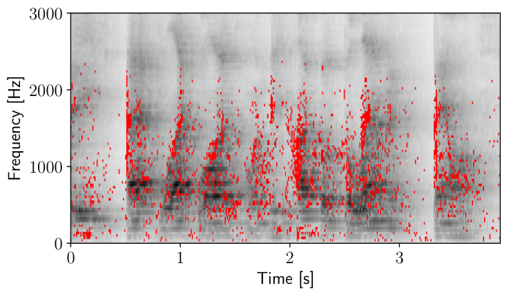
Figure 2: Evaluation of confidence weights predicted by C-SL: Scatter plot of time-frequency bins (red pixels) with estimated confidence in the 95-th percentile overlaid on a sample spectrogram. Sensor-frame direction errors σ⁡(rs,r~^s)\sigma(r^{s},\mathchoice{\hat{\hbox{$\displaystyle\tilde{r}$}}}{\hat{\hbox{$\textstyle\tilde{r}$}}}{\hat{\hbox{$\scriptstyle\tilde{r}$}}}{\hat{\hbox{$\scriptscriptstyle\tilde{r}$}}}^{s}) vs. predicted confidence ‖r~s‖\left\lVert\tilde{r}^{s}\right\rVert estimated by C-SL averaged over percentile groups of time-frequency bins in the CmixedC_{\text{mixed}} dataset.

In the second experiment, we performed an assessment of the confidence weights predicted by C-SL. To find these weights, we calculated ℓ2\ell_{2} norm of the MLP output for all time-frequency bins extracted from the test dataset in CmixedC_{\text{mixed}} condition. Figure 2 illustrates the scatter plot of the bins with weights in the 95-percentile for a highly reverberated session in this dataset (T60=750 msT_{60}=$750\text{\,}\mathrm{m}\mathrm{s}$) overlaid on the session spectrogram. As expected, majority of these bins are concentrated around signal onsets at frequencies carrying higher energy. We also examined how these confidence scores are related to sensor frame estimation errors calculated by σ⁡(rs,r~^s)\sigma(r^{s},\hat{\tilde{r}}^{s}). Figure 2 shows error curve vs. confidence weights found using a quantile-based binning of time-frequency bins. The monotonic decrease in average errors indicates that the model has successfully learned to predict uncertainty in estimations.

In our last experiment, we investigated application of C-SL at inference time in a multi-source environment. In such conditions, it can be assumed that each time-frequency bin is dominated by one source, therefore finding location of the sources can be cast as a clustering task where time-frequency bins are assigned to different clusters based on their predicted world frame direction. While many approaches could be used for the clustering, we opted for a non-parametric kernel density estimation (KDE) based technique to detect dominant directions. In this method, given estimated world-frame directions for an ensemble of bins within a window, we first approximate the weighted density of directions on a uniform grid (same as the one used in the first experiment) by ψn(rj)=∑k,n′∈In‖r~k,n′w‖e−σ(rj,r~^wk,n′)/α\psi_{n}(r_{j})=\sum\limits_{k,n^{\prime}\in I_{n}}\left\lVert\tilde{r}^{w}_{k,n^{\prime}}\right\rVert e^{-\sigma(r_{j},\hat{\tilde{r}}^{w}_{k,n^{\prime}})/\alpha} where we set α=1​°\alpha=$$ as the bandwidth of the kernel. Given the maximum number of sources NsrcN_{\text{src}}, we then find local maxima of function ψ\psi on the grid, and pick NsrcN_{\text{src}} peaks with highest density as the estimates of source direction for the window.

[Uncaptioned image] Figure 3: Log-scale kernel density values estimated by C-SL for a sample time window of length 200 ms200\text{\,}\mathrm{m}\mathrm{s}. (⋅{\color[rgb]{1,0,0}\Bigcdot}) and (×{\color[rgb]{0,0.88,0}\boldsymbol{\times}}) depict predicted and ground truth source locations on the grid.
Table 2: C-SL estimation errors (in degree) in two-speaker scenario computed for different window lengths in anechoic condition.
Lwin​(s)L_{\text{win}}($\mathrm{s}$) dw-chamferd_{\text{w-chamfer}}
0.05 9.87​±0.119.87{\color[rgb]{0.5,0.5,0.5}\mathchoice{\raisebox{-0.64655pt}{\resizebox{1610148}{327680}{\hbox{\raisebox{0.83333pt}{$\displaystyle\pm 0.11$}}}}}{\raisebox{-0.64655pt}{\resizebox{1610148}{327680}{\hbox{\raisebox{0.83333pt}{$\textstyle\pm 0.11$}}}}}{\raisebox{-0.92365pt}{\resizebox{1930967}{327680}{\hbox{\raisebox{0.83334pt}{$\scriptstyle\pm 0.11$}}}}}{\raisebox{-1.25002pt}{\resizebox{2334712}{327680}{\hbox{\raisebox{0.83336pt}{$\scriptscriptstyle\pm 0.11$}}}}}}
0.2 4.26​±0.134.26{\color[rgb]{0.5,0.5,0.5}\mathchoice{\raisebox{-0.64655pt}{\resizebox{1610148}{327680}{\hbox{\raisebox{0.83333pt}{$\displaystyle\pm 0.13$}}}}}{\raisebox{-0.64655pt}{\resizebox{1610148}{327680}{\hbox{\raisebox{0.83333pt}{$\textstyle\pm 0.13$}}}}}{\raisebox{-0.92365pt}{\resizebox{1930967}{327680}{\hbox{\raisebox{0.83334pt}{$\scriptstyle\pm 0.13$}}}}}{\raisebox{-1.25002pt}{\resizebox{2334712}{327680}{\hbox{\raisebox{0.83336pt}{$\scriptscriptstyle\pm 0.13$}}}}}}
0.5 2.85​±0.152.85{\color[rgb]{0.5,0.5,0.5}\mathchoice{\raisebox{-0.64655pt}{\resizebox{1610148}{327680}{\hbox{\raisebox{0.83333pt}{$\displaystyle\pm 0.15$}}}}}{\raisebox{-0.64655pt}{\resizebox{1610148}{327680}{\hbox{\raisebox{0.83333pt}{$\textstyle\pm 0.15$}}}}}{\raisebox{-0.92365pt}{\resizebox{1930967}{327680}{\hbox{\raisebox{0.83334pt}{$\scriptstyle\pm 0.15$}}}}}{\raisebox{-1.25002pt}{\resizebox{2334712}{327680}{\hbox{\raisebox{0.83336pt}{$\scriptscriptstyle\pm 0.15$}}}}}}
1.0 2.22​±0.152.22{\color[rgb]{0.5,0.5,0.5}\mathchoice{\raisebox{-0.64655pt}{\resizebox{1610148}{327680}{\hbox{\raisebox{0.83333pt}{$\displaystyle\pm 0.15$}}}}}{\raisebox{-0.64655pt}{\resizebox{1610148}{327680}{\hbox{\raisebox{0.83333pt}{$\textstyle\pm 0.15$}}}}}{\raisebox{-0.92365pt}{\resizebox{1930967}{327680}{\hbox{\raisebox{0.83334pt}{$\scriptstyle\pm 0.15$}}}}}{\raisebox{-1.25002pt}{\resizebox{2334712}{327680}{\hbox{\raisebox{0.83336pt}{$\scriptscriptstyle\pm 0.15$}}}}}}

For this experiment, we created a new test dataset in anechoic condition consisting of 600 sessions each with two sources. To generate each session, two sentences were randomly selected from the test split we generated before and spatialized according to random independent locations selected for each of the sources and motions of the array similar to the single source condition. Spatialized sounds from the two sources were then added together (after padding the shorter one with zeros at the end) to generate the recordings at each microphone. Finally, time windows extracted from these recordings with at least one source present were used to evaluate the performance of C-SL in a two-speaker condition. Figure 3 shows log-scale grid densities calculated for a sample input window and the corresponding predicted and ground truth pairs of directions. As it can be seen, the identified peaks are very sharp and lie close to ground-truth locations of the sources, a trend that we found to be generally true when using C-SL. In order to quantify the error between the predicted set of sensor frame directions and their ground truth values, denoted by R¯s\bar{R}^{s} and RsR^{s}, we used a weighted version of Chamfer distance to match directions in the two sets and measure the deviation between them as following:

dw-chamfer​(R¯s,Rs)=\displaystyle d_{\text{w-chamfer}}(\bar{R}^{s},R^{s})= 1|Rs|​∑r∈Rsminr′∈R¯s⁡σ⁡(r,r′)\displaystyle\frac{1}{\lvert R^{s}\rvert}\sum\limits_{r\in R^{s}}\min\limits_{r^{\prime}\in\bar{R}^{s}}\sigma(r,r^{\prime})
+\displaystyle+ 1∑r′∈R¯sψ⁡(r′)​∑r′∈R¯sψ⁡(r′)​minr∈Rs⁡σ⁡(r,r′)(8)\displaystyle\frac{1}{\sum\limits_{r^{\prime}\in\bar{R}^{s}}\psi(r^{\prime})}\sum\limits_{r^{\prime}\in\bar{R}^{s}}\psi(r^{\prime})\min\limits_{r\in R^{s}}\sigma(r,r^{\prime})\qquad(8)

The weighting can be thought of as a mechanism to filter out spurious peaks based on their density without having to choose thresholds. We calculated values of this metric for different window durations ranging from 50 ms to 1000 ms50\text{\,}\mathrm{m}\mathrm{s}1000\text{\,}\mathrm{m}\mathrm{s}. Results, shown in Table 2, demonstrate that in conjunction with the appropriate clustering scheme C-SL can also be utilized in multi-source environments.

4 Conclusion

In this paper, we presented Contrastive Sound Localization (C-SL), a framework for learning acoustic-spatial mappings from unlabled data collected by microphone arrays of arbitrary geometry. C-SL combines contrastive learning and acoustic-inertial sensor fusion to simultaneously calibrate the array and estimate DOAs in a self-supervised manner. Our evaluations demonstrate that, by leveraging array movements, C-SL can localize sounds in a wide range of conditions with no additional information about the array or the sources available The relaxed data collection, simplicity and low computational requirements to train the model, together with the encouraging results in challenging conditions are advancements offered by C-SL that pave the way toward personalized hearing applications.

References

  • [1] J. Blauert, Spatial hearing: the psychophysics of human sound localization. MIT press, 1997.
  • [2] H. Wallach, “The role of head movements and vestibular and visual cues in sound localization.,” Journal of Experimental Psychology, vol. 27, no. 4, p. 339, 1940.
  • [3] D. Genzel, U. Firzlaff, L. Wiegrebe, and P. R. MacNeilage, “Dependence of auditory spatial updating on vestibular, proprioceptive, and efference copy signals,” Journal of neurophysiology, vol. 116, no. 2, pp. 765–775, 2016.
  • [4] B. G. Shinn-Cunningham, N. I. Durlach, and R. M. Held, “Adapting to supernormal auditory localization cues. i. bias and resolution,” The Journal of the Acoustical Society of America, vol. 103, no. 6, pp. 3656–3666, 1998.
  • [5] J. H. DiBiase, A high-accuracy, low-latency technique for talker localization in reverberant environments using microphone arrays. Brown University Providence, RI, 2000.
  • [6] R. Schmidt, “Multiple emitter location and signal parameter estimation,” IEEE transactions on antennas and propagation, vol. 34, no. 3, pp. 276–280, 1986.
  • [7] R. Roden, N. Moritz, S. Gerlach, S. Weinzierl, and S. Goetze, “On sound source localization of speech signals using deep neural networks,” 2015.
  • [8] X. Xiao, S. Zhao, X. Zhong, D. L. Jones, E. S. Chng, and H. Li, “A learning-based approach to direction of arrival estimation in noisy and reverberant environments,” in 2015 IEEE International Conference on Acoustics, Speech and Signal Processing (ICASSP), pp. 2814–2818, IEEE, 2015.
  • [9] S. Chakrabarty and E. A. Habets, “Broadband doa estimation using convolutional neural networks trained with noise signals,” in 2017 IEEE Workshop on Applications of Signal Processing to Audio and Acoustics (WASPAA), pp. 136–140, IEEE, 2017.
  • [10] Z.-Q. Wang, X. Zhang, and D. Wang, “Robust speaker localization guided by deep learning-based time-frequency masking,” IEEE/ACM Transactions on Audio, Speech, and Language Processing, vol. 27, no. 1, pp. 178–188, 2018.
  • [11] S. Adavanne, A. Politis, and T. Virtanen, “Direction of arrival estimation for multiple sound sources using convolutional recurrent neural network,” in 2018 26th European Signal Processing Conference (EUSIPCO), pp. 1462–1466, IEEE, 2018.
  • [12] D. Comminiello, M. Lella, S. Scardapane, and A. Uncini, “Quaternion convolutional neural networks for detection and localization of 3d sound events,” in ICASSP 2019-2019 IEEE International Conference on Acoustics, Speech and Signal Processing (ICASSP), pp. 8533–8537, IEEE, 2019.
  • [13] A. v. d. Oord, Y. Li, and O. Vinyals, “Representation learning with contrastive predictive coding,” arXiv preprint arXiv:1807.03748, 2018.
  • [14] T. Chen, S. Kornblith, M. Norouzi, and G. Hinton, “A simple framework for contrastive learning of visual representations,” arXiv preprint arXiv:2002.05709, 2020.
  • [15] Y. Tian, D. Krishnan, and P. Isola, “Contrastive representation distillation,” arXiv preprint arXiv:1910.10699, 2019.
  • [16] P. Sermanet, C. Lynch, Y. Chebotar, J. Hsu, E. Jang, S. Schaal, S. Levine, and G. Brain, “Time-contrastive networks: Self-supervised learning from video,” in 2018 IEEE International Conference on Robotics and Automation (ICRA), pp. 1134–1141, IEEE, 2018.
  • [17] S. Pirk, M. Khansari, Y. Bai, C. Lynch, and P. Sermanet, “Online object representations with contrastive learning,” arXiv preprint arXiv:1906.04312, 2019.
  • [18] H. Zhao, C. Gan, A. Rouditchenko, C. Vondrick, J. McDermott, and A. Torralba, “The sound of pixels,” in Proceedings of the European Conference on Computer Vision (ECCV), pp. 570–586, 2018.
  • [19] A. Owens and A. A. Efros, “Audio-visual scene analysis with self-supervised multisensory features,” in Proceedings of the European Conference on Computer Vision (ECCV), pp. 631–648, 2018.
  • [20] C. Gan, H. Zhao, P. Chen, D. Cox, and A. Torralba, “Self-supervised moving vehicle tracking with stereo sound,” in Proceedings of the IEEE International Conference on Computer Vision, pp. 7053–7062, 2019.
  • [21] H. Liu, Z. Zhang, Y. Zhu, and S.-C. Zhu, “Self-supervised incremental learning for sound source localization in complex indoor environment,” in 2019 International Conference on Robotics and Automation (ICRA), pp. 2599–2605, IEEE, 2019.
  • [22] S. Kumar, W. Sedley, K. V. Nourski, H. Kawasaki, H. Oya, R. D. Patterson, M. A. Howard III, K. J. Friston, and T. D. Griffiths, “Predictive coding and pitch processing in the auditory cortex,” Journal of Cognitive Neuroscience, vol. 23, no. 10, pp. 3084–3094, 2011.
  • [23] Y. Almalioglu, M. Turan, A. E. Sari, M. R. U. Saputra, P. P. de Gusmão, A. Markham, and N. Trigoni, “Selfvio: Self-supervised deep monocular visual-inertial odometry and depth estimation,” arXiv preprint arXiv:1911.09968, 2019.
  • [24] T. Qin, P. Li, and S. Shen, “Vins-mono: A robust and versatile monocular visual-inertial state estimator,” IEEE Transactions on Robotics, vol. 34, no. 4, pp. 1004–1020, 2018.
  • [25] R. Mur-Artal and J. D. Tardós, “Visual-inertial monocular slam with map reuse,” IEEE Robotics and Automation Letters, vol. 2, no. 2, pp. 796–803, 2017.
  • [26] S. Madgwick, “An efficient orientation filter for inertial and inertial/magnetic sensor arrays,” Report x-io and University of Bristol (UK), vol. 25, pp. 113–118, 2010.
  • [27] J. B. Kuipers et al., Quaternions and rotation sequences, vol. 66. Princeton university press Princeton, 1999.
  • [28] K. Wu, V. G. Reju, and A. W. Khong, “Multisource doa estimation in a reverberant environment using a single acoustic vector sensor,” IEEE/ACM Transactions on Audio, Speech, and Language Processing, vol. 26, no. 10, pp. 1848–1859, 2018.
  • [29] T. Salimans and D. P. Kingma, “Weight normalization: A simple reparameterization to accelerate training of deep neural networks,” in Advances in neural information processing systems, pp. 901–909, 2016.
  • [30] D. Diaz-Guerra, A. Miguel, and J. R. Beltran, “gpurir: A python library for room impulse response simulation with gpu acceleration,” arXiv preprint arXiv:1810.11359, 2018.
  • [31] J. B. Allen and D. A. Berkley, “Image method for efficiently simulating small-room acoustics,” The Journal of the Acoustical Society of America, vol. 65, no. 4, pp. 943–950, 1979.
  • [32] J. S. Garofolo, L. F. Lamel, W. M. Fisher, J. G. Fiscus, D. S. Pallett, and N. L. Dahlgren, “Darpa timit acoustic phonetic continuous speech corpus cdrom,” 1993.
  • [33] D. P. Kingma and J. Ba, “Adam: A method for stochastic optimization,” arXiv preprint arXiv:1412.6980, 2014.
  • [34] V. Tourbabin, J. Donley, B. Rafaely, and R. Mehra, “Direction of arrival estimation in highly reverberant environments using soft time-frequency mask,” in 2019 IEEE Workshop on Applications of Signal Processing to Audio and Acoustics (WASPAA), pp. 383–387, IEEE, 2019.

Appendix

Theorem.

Given bijective functions g,f:A→𝕊2g,f\colon A\rightarrow\mathbb{S}^{2} defined on the non-empty set AA and the constraint CC: ∀x,y∈A,∀Rx,Ry∈S​O​(3):Rx​f​(x)=Ry​f​(y)⇔Rx​g​(x)=Ry​g​(y)\forall x,y\in A,\forall R_{x},R_{y}\in SO(3)\colon R_{x}f(x)=R_{y}f(y)\iff R_{x}g(x)=R_{y}g(y), CC holds if and only if f=±gf=\pm g.

Proof.

It is trivial to show CC holds when f=±gf=\pm g.
Now let θ⁡(R)\theta(R) denote the rotation angle corresponding to rotation matrix RR. It can be shown that:

∀u,v∈𝕊2:⟨u,v⟩=maxR∈S​O​(3):R​u=vcos(θ(R))\forall u,v\in\mathbb{S}^{2}\colon\langle u,v\rangle=\max\limits_{R\in SO(3)\colon Ru=v}\cos{(\theta(R))} (1)

Using this we can show that if CC holds:

∀x,y∈A:⟨f⁡(x),f⁡(y)⟩=⟨g⁡(x),g⁡(y)⟩\forall x,y\in A:\langle f(x),f(y)\rangle=\langle g(x),g(y)\rangle\\ (2)

By setting values of yy in (2) to a1=g−1​(i^)a_{1}=g^{-1}(\bm{\hat{\textbf{i}}}), a2=g−1​(j^)a_{2}=g^{-1}(\bm{\hat{\textbf{j}}}), and a3=g−1​(k^)a_{3}=g^{-1}(\bm{\hat{\textbf{k}}}) we get:

g=P​fg=Pf (3)

where

P=[f⁡(a1)f⁡(a2)f⁡(a3)]TP=\left[\begin{array}[]{@{}c|c|c@{}}f(a_{1})&f(a_{2})&f(a_{3})\end{array}\right]^{T} (4)

Furthermore since (3) also holds for a1a_{1}, a2a_{2} and a3a_{3} it can be shown that:

PT​P=P​PT=IP^{T}P=PP^{T}=I (5)

By plugging (3) into CC and setting R=Ry−1​RxR=R_{y}^{-1}R_{x}, we will get:

∀x,y∈A,∀R∈S​O​(3):R​f​(x)=f⁡(y)⇔R​P​f​(x)=P​f​(y)\forall x,y\in A,\forall R\in SO(3):Rf(x)=f(y)\iff RPf(x)=Pf(y) (6)

which is equivalent to

∀R∈S​O​(3):R​P=P​R\forall R\in SO(3):RP=PR (7)

(5) and (7) imply that P=±IP=\pm I. Therefore f=±gf=\pm g. ∎