Online Page Migration with ML Advice
Abstract
We consider online algorithms for the page migration problem that use predictions, potentially imperfect, to improve their performance. The best known online algorithms for this problem, due to Westbrook’94 and Bienkowski et al’17, have competitive ratios strictly bounded away from 1. In contrast, we show that if the algorithm is given a prediction of the input sequence, then it can achieve a competitive ratio that tends to as the prediction error rate tends to . Specifically, the competitive ratio is equal to , where is the prediction error rate. We also design a “fallback option” that ensures that the competitive ratio of the algorithm for any input sequence is at most . Our result adds to the recent body of work that uses machine learning to improve the performance of “classic” algorithms.
1 Introduction
Recently, there has been a lot of interest in using machine learning to design improved algorithms for various computational problems. This includes work on data structures [KBC+18, Mit18], online algorithms [LV18, PSK18, GP19a, Roh20], combinatorial optimization [KDZ+17, BDSV18], similarity search [WLKC16], compressive sensing [MPB15, BJPD17] and streaming algorithms [HIKV19]. This body of work is motivated by the fact that modern machine learning methods are capable of discovering subtle structure in collections of input data, which can be utilized to improve the performance of algorithms that operate on similar data.
In this paper we focus on learning-augmented online algorithms. An on-line algorithm makes non-revocable decisions based only on the part of the input seen so far, without any knowledge of the future. It is thus natural to consider a relaxation of the model where the algorithm has access to (imperfect) predictors of the future input that could be used to improve the algorithm performance. Over the last couple of years this line of research has attracted growing attention in the machine learning and algorithms literature, for classical on-line problems such as caching [LV18, Roh20], ski-rental and scheduling [PSK18, GP19b, LLMV20] and graph matching [KPS+19]. Interestingly, most of the aforementioned works conclude that the ‘‘optimistic’’ strategy of simply following the predictions, i.e., executing the optimal solution computed off-line for the predicted input, can lead to a highly sub-optimal performance even if the prediction error is small.11 1 To the best of our knowledge the only problem for which this strategy is known to result in an optimal algorithm is the online bipartite matching, see Section 1.1 for more details. For instance, for caching, even a single misprediction can lead to an unbounded competitive ratio [LV18].
In this paper we show that, perhaps surprisingly, the aforementioned “optimistic” strategy leads to near-optimal performance for some well-studied on-line problems. We focus on the problem of page migration [BS89] (a.k.a. file migration [Bie12] or 1-server with excursions [MMS90]). Here, the algorithm is given a sequence of points (called requests) from a metric space , in an online fashion. The state of the algorithm is also a point from . Given the next request , the algorithm moves to its next state (at the cost of , where is a parameter), and then “satisfies” the request (at the cost of ). The objective is to satisfy all requests while minimizing the total cost. The problem has been a focus on a large body of research, see e.g., [ABF93, Wes94, CLRW97, BCI97, KM16, BBM17]. The best known algorithms for this problem have competitive ratios of (a deterministic algorithm due to [BBM17]), (a randomized algorithm against adaptive adversaries due to [Wes94]) and (a randomized algorithm against oblivious adversaries due to [Wes94]). The original paper [BS89] also showed that the competitive ratio of any deterministic algorithm must be at least , which was recently improved to for some by [Mat15].
Our results
Suppose that we are given a predicted request sequence that, in each interval of length , differs from the actual sequence on at most a fraction of positions, where are the parameters (note that the lower the values of and are, the stronger our assumption is). Under this assumption we show that the optimal off-line solution for is a -competitive solution for as long as the parameter is a small enough constant. Thus, the competitive ratio of this prediction-based algorithm improves over the state of the art even if the number of errors is linear in the sequence length, and tends to when the error rate tends to .22 2 Note that if each interval of length has at most a fraction of of errors, then it is also the case that each interval of length has at most a fraction of of errors. Thus, if tends to , the competitive ratio tends to even if the interval length remains fixed. Furthermore, to make the algorithm robust, we also design a “fallback option”, which is triggered if the input sequence violates the aforementioned assumption (i.e., if the fraction of errors in the suffix of the current input sequence exceeds ). The fallback option ensures that the competitive ratio of the algorithm for any input sequence is at most . Thus, our final algorithm produces a near-optimal solution if the prediction error is small, while guaranteeing a constant competitive ratio otherwise.
For the case when the underlying metric is uniform, i.e., all distances between distinct points are equal to , we further improve the competitive ratio to under the assumption that each interval of length differs from the actual sequence in at most positions. That is, the parameter is not needed in this case. Moreover, any algorithm has a competitive ratio of at least .
It is natural to wonder whether the same guarantees hold even when the predicted sequence differs from the actual sequence on at most a fraction of positions distributed arbitrarily over , as opposed to over chunks of length . We construct a simple example that shows that such a relaxed assumption results in the same lower bound as for the classical problem.
1.1 Related Work
Multiple variations of the page migration problem have been studied over the years. For example, if the page can be copied as well as moved, the problem has been studied under the name of file allocation, see e.g., [BFR95, ABF03, LRWY98]. Other formulations add constraints on nodes capacities, allow dynamically changing networks etc. See the survey [Bie12] for an overview.
There is a large body of work concerning on-line algorithms working under stochastic or probabilistic assumptions about the input [Unc16]. In contrast, in this paper we do not make such assumptions, and allow worst case prediction errors (similarly to [LV18, KPS+19, PSK18]). Among these works, our prediction error model (bounding the fraction of mispredicted requests) is most similar to the “agnostic” model defined in [KPS+19]. The latter paper considers on-line matching in bipartite graphs, where a prediction of the graph is given in advance, but the final input graph can deviate from the prediction on vertices. Since each vertex impacts at most one matching edge, it directly follows that errors reduce the matching size by at most . In contrast, in our case a single error can affect the cost of the optimum solution by an arbitrary amount. Thus, our analysis requires a more detailed understanding of the properties of the optimal solution.
Multiple papers studied on-line algorithms that are given a small number of bits of advice [BFK+17] and show that, in many scenarios, this can improve their competitive ratios. Those algorithms, however, typically assume that the advice is error-free.
2 Preliminaries
Page Migration
In the classical version, the algorithm is given a sequence of points (called requests) from a metric space , in an online fashion. The state of the algorithm (i.e., the page), is also a point from . Given the next request , the algorithm moves to its next state (at the cost of , where is a parameter), and then “satisfies” the request (at the cost of ). The objective is to satisfy all requests while minimizing the total cost. We can consider a version of this problem where the algorithm is given, prior to the arrival of the requests, a predicted sequence . The (final) sequence is generated adversarially from and an arbitrary adversarial sequence . That is either or . If we do not make any assumptions on how well is predicted by , then the problem is no easier than the classical online version. On the other hand, if , then one obtains an optimal online algorithm, by simply computing the optimal offline algorithm. The interesting regime lies in between these two cases. We will make the following assumption throughout the paper, which roughly speaking demands that a fraction of the input is correctly predicted and that the fraction of errors is somewhat spread out.
Definition 1 (Number of mismatches ).
Let be an interval of indices. We define to be the number of mismatches between and within the interval .
Assumption 1.
Consider an interval of of length . For any it holds .
Remark 1.
Relaxing 1 by allowing the adversary to change an arbitrary fraction of the input results in the same lower bound as for the classical problem. To see this, consider an arbitrary instance on elements that gives a lower bound of in the classical problem. Call this sequence of elements adversarial. Let consists of elements being equal to the starting point. That is, is simply the starting position replicated times. Let be equal to the sequence whose suffix of length is replaced by the adversarial sequence. Now, on defined in this way no algorithm can be better than -competitive. Hence, in general this relaxation of 1 gives no advantage.
Our main results hold for general metric space, where for all all of the following hold: , for , , and . We obtain better results for uniform metric space, where, for .
Notation
Given a sequence , we use to denote the -th element of . For integers and , such that , we use to denote the subsequence of consisting of the elements .
For a fixed algorithm, let be the position of the page at time . In particular, denotes the start position for all algorithms.
Given an algorithm that pays cost for serving requests, we denote by the cost paid by during the interval . We sometimes abuse notation and write as a shorthand for . In particular, denotes as well as . This notation is the most often used in the context of our algorithm ALG and the optimal solution OPT, whose total serving costs are and , respectively.
3 Proof Overview
Our two main contributions are: algorithm ALG that is -competitive provided 1; and, a black-box reduction from ALG to a -competitive algorithm when 1 does not hold. In Section 3.1 we present an overview of ALG, while an overview of is given in Section 3.2.
3.1 ALG under assumption 1
Algorithm ALG (given as Algorithm 1) simply computes the optimal offline solution and moves pages accordingly.
Input The number of the next request.
Output and are sequences as defined in Section 2.
The main challenge in proving that ALG still performs well in the online setting lies in leveraging the optimality of ALG with respect to the offline sequence. The reason for this is that, due to and not being identical, OPT and ALG may be on different page locations throughout all the requests. In addition to that, we have no control over which fraction of any interval of length is changed nor to what it is changed. In particular, if , then and could be very far from each other. To circumvent this, we use the following way to argue about the offline optimality, that is, about the optimality computed with respect to .
We think of ALG (OPT, respectively) as a sequence of page locations that are defined with respect to (, respectively). These page locations do not change even if, for instance, the -th online request to ALG deviates from . Let (, respectively) be the cost of ALG (OPT, respectively) serving requests given by . Similarly, let (, respectively) be the cost of ALG (OPT, respectively) for serving the oracle subsequence . In particular, is the cost of ALG (optimal on ) on the final sequence , whereas is the cost of the optimal algorithm for on the predicted sequence . It is convenient to think of as the ‘evil twin’ of .
We have, due to optimality of ALG on the offline sequence,
| (1) |
The intuition behind this is best explained pictorially, which we do in Fig. 1. Here ALG is at and OPT is at . In the depicted example a request is moved from to . This causes to increase, however, at the same time, decreases by almost the same amount.33 3 We oversimplified here, since the right hand side of (1) only holds for the sum of all points, but a similar argument can be made for a single requests. In fact, one can show that for such a moved page the right hand side of Eq. 1 will increase by no more than . For pages that are not moved, i.e., , the costs of ALG and OPT do not change. It remains to bound , which we do next. By triangle inequality, it holds that
| (2) |
Consider an interval . Let be the total sum of moving costs for both OPT and ALG for the requests in the interval . As a reminder (see Definition 1), for a given interval , is the number of mismatches between and within . From Eq. 2, we derive
| (3) |
We would like the right hand side of Eq. 3 to be small, implying that is small as well. To understand the nature of the right hand side of Eq. 3 and what is required for it to be small, assume for a moment that . Then, the rest of the summation telescopes to , and Eq. 3 reduces to . Now, if is sufficiently small, e.g., , then we are able to upper-bound Eq. 3 by and derive
which gives the desired competitive factor.
So, to utilize Eq. 3, in our proof we will focus on showing that is sufficiently smaller than . However, this can be challenging as OPT is allowed to move often, potentially on every request which results in being very small. But, if is too small, then 1 gives no information about . However, if intervals would be large enough, e.g., at least for some positive constant , then from 1 we would be able to conclude that . Since in principle OPT can move in every step, we design ‘lazy’ versions of OPT and ALG that only move times in any interval of length . This will enable us to argue that is not too small. It turns out that the respective competitive factors of the lazy versions with respect to the original versions is very close, allowing us prove
3.2 , a robust version of ALG
We now describe . This algorithm follows a “lazy” variant of ALG as long as 1 holds, and otherwise switches to . Instead of using ALG directly, we use a ‘lazy’ version of ALG that works as follows: Follow the optimal offline solution given by ALG with a delay of steps. Let be the corresponding algorithm. We point out that performing some delay with respect to ALG is crucial here. To see that, consider the following example in the case of uniform metric spaces: and , and let the starting location be . According to ALG, the page should be moved from to in the very beginning, incurring the cost of . On the other hand, OPT never moves from . If would follow ALG until it realizes that the fraction of errors is too high, it would already pay the cost of at least , leading to an unbounded competitive ratio. However, if delays following ALG, then it gets some “slack” in verifying whether the predicted sequence properly predicts requests or not. As a result, when 1 holds, this delay increases the overall serving cost by a factor , but in turn achieves a bounded competitive ratio when this assumption does not hold.
While serving requests, also maintains the execution of , i.e., maintains where would be at a given point in time, in case a fallback is needed. Now simply executes unless we find a violation of 1 is detected. Once such a violation is detected, the algorithm switches to by moving its location to ’s current location. From there on is executed.
We now present the intuition behind the proof for the competitive factor of the algorithm.
Case when 1 holds.
In this case is , and the analysis boils down to proving competitive ratio of . We show that is -competitive to ALG, which is, as we argued in the previous section, competitive to OPT. To see this, we employ the following charging argument: whenever ALG moves from to it pays . The lazy algorithm eventually pays the same moving cost of less.
However, in addition, the serving cost of for each of the requests is potentially increased, as is not at the same location as ALG. Nevertheless, by triangle inequality, the cost due to the movement from to of ALG reflect to an increase in the serving cost of by at most . In total over all the requests and per each move of ALG from to , pays at most extra cost compared to ALG. Considering all migrations, this gives a competitive factor.
Case when 1 is violated.
The case where 1 is violated (say at time ) is considerably more involved. We then have
and we seek to upper-bound each of these terms by . While the upper-bound holds directly for , showing the upper-bound for other terms is more challenging.
The key insight is that, due to the optimality of ALG,
| (4) |
which can be proven as follows. If ALG migrates its page to a location that is far from the starting location , then there have to be, even when taking into account noise, at least page requests that are far from . OPT also has to serve these requests (either remotely or by moving), and hence has to pay a cost of at least . Equipped with this idea, we can now bound in terms of . To bound we need one more idea. Namely, we compare to the optimal solution that has a constraint to be at the same position as at time . A formal analysis is given in Section 5.
4 The Analysis of ALG
Now we analyze ALG (Algorithm 1). As discussed in Section 3.1, our main objective is to establish Eq. 3, which we do in Section 4.1. That upper-bound will be directly used to obtain our result for uniform metric spaces, as we present in Section 4.2. To construct our algorithm for general-metric spaces, in Section 4.3 we build on ALG by first designing its “lazy” variant. As the final result, we show the following. Recall that is the fraction of symbols that the adversary is allowed to change in any sequence of length of the predicted sequence.
Theorem 1.
If 1 holds with respect to parameter , then we obtain the following results:
- (A)
There exists a -competitive algorithm for the online page migration problem.
- (B)
There exists a -competitive algorithm for the online page migration problem in uniform metric spaces.
Note that Theorem 1 is asymptotically optimal with respect to . Namely, any algorithm is at least competitive; even in the uniform metric case. To see this consider the following binary example where the algorithm starts at position . The advice is . The final sequence is
In the first case OPT simply stays at since moving costs ; in the second case, OPT goes immediately to . Note that ALG can only distinguish between the sequences after steps at which point it is doomed to have an additional cost of with probability at least depending on the sequence .
4.1 Establishing Eq. 3
In our proofs we will use the following corollary of 1.
Corollary 1.
If 1 holds, then for any interval of length it holds .
Proof.
This statement follows from the fact that each such can be subdivided into intervals of length exactly and at most one interval of length less than . On one hand, the total number of mismatches for these intervals of length exactly is upper-bounded by . On the other hand, since is a subinterval of an interval of length , it holds . The claim now follows. ∎
Most of our analysis in this section proceeds by reasoning about intervals where neither ALG nor OPT moves. Let be the time steps at which either OPT or ALG move. The final product of this section will be an upper-bound on as given by Eq. 344 4 As a reminder, (, respectively) is the cost of ALG (OPT, respectively) at time for the sequence ., i.e.,
We begin by rewriting and upper-bounding as follows
| (5) |
where we used that as is the optimum for . Consider a fixed interval . Then, by triangle inequality, it holds
| (6) |
Let be the sum of moving costs for OPT and ALG in . Note that
| (7) |
where the inequality comes from Eq. 6 applied to every time step in ( and the fact that ALG or OPT must have moved inducing a cost of at least . The following notation is used to represent the difference between serving and by ALG
Note that this holds even when ALG moves since the moving costs for the oracle sequence and on the final sequence are the same and therefore cancel each other out. Similarly to , let
Consider now any . By triangle inequality we have
| (8) |
Let , where by definition. Note that
Recall that, for a given interval the function denotes the number of mismatches between and within (see Definition 1). Now, as for such that we have , the last chain of inequalities further implies
| (9) |
This establishes the desired upper-bound on . As discussed in Section 3.1, this upper-bound is used to derive our non-robust results for uniform (Section 4.2) and general (Section 4.3) metric spaces. The main task in those two sections will be to show that is sufficiently smaller than .
4.2 Uniform Metric Spaces – Theorem 1 (B)
We now use the upper-bound on given by Eq. 9 to show that ALG is -competitive under 1, i.e., we show Theorem 1 (A). We distinguish between two cases: ; and .
Case .
In this case, by Corollary 1 we have . Plugging this into Eq. 9 we derive
Case .
We proceed by upper-bounding all the terms in Eq. 9. As the interval is a subinterval of , we have
Also, observe that trivially it holds
| (10) |
Combining the derived upper-bounds, we establish
| (11) | ||||
| (12) |
To conclude this case, note that by definition either ALG or OPT moves within , incurring the cost of at least . Therefore, . This together with Eq. 12 implies
Combining the two cases.
We have concluded that in either case it holds and hence we derive
This concludes the analysis for uniform metric spaces.
4.3 General Metric Spaces – Theorem 1 (A)
As in the uniform case, our goal for general metric spaces is to use Eq. 3 for proving the advertised competitive ratio. However, as we discussed in Section 3.1, the main challenge in applying Eq. 3 lies in upper-bounding the ratio between and by a small constant, ideally much smaller than . Unfortunately, this ratio can be as large as as OPT (or ALG) could possibly move on every single request. To see that, consider the scenario in which all the requests are on the -axis and are requested in their increasing order of their location. Then, for all but potentially the last requests, OPT would move from request to request. To bypass this behavior of OPT and ALG, we define and analyze their “lazy” variants, i.e., variants in which OPT and ALG are allowed to move only at the -th request when is a multiple of . We now state the algorithm.
4.3.1 Our Algorithm
We use the following algorithm : Compute the optimal offline solution (on ) while only moving on multiples of . Let be the cost of the solution and let be the cost of the solution on . Note that there can be better offline algorithms for , however has the minimal cost among all online algorithms that are only allowed to move every multiple of .
4.3.2 Proof
We also need to consider a lazy version of OPT, which we do in the following lemma. There we show that making any algorithm lazy does not increase the cost by more than a factor of . In particular, we will show . Let and denote their costs at time .
Lemma 1.
Let . Consider an arbitrary prefix of length of a sequence of requests. Let be the cost of any algorithm serving . Let be the cost of the algorithm that has to move at every time step that is a multiple of (and is not allowed to move at any other time step), and to move to the position where is at that time step. Then, we have
Proof.
Let be the distance of the -th move and be the cost for serving the -th request remotely. Then,
Now we relate and . has two components: the moving cost and the cost for serving remotely. By triangle inequality, the moving cost is upper-bounded by . Consider now interval for some integer . To serve point remotely, the cost is, by triangle inequality, at most the cost of plus the cost of traversing all the points with indices in where has moved to. Thus the cost per request is upper-bounded by . Note that the summation is charged to requests. Hence, summing over all the intervals gives
∎
Define as the cost of the optimal algorithm for that is allowed to move only at time steps which are multiple of . Similarly as in Lemma 1, we have . Thus,
| (13) |
Now we need to upper-bound . We will do that by showing that the same statements as we developed in Section 4.1 hold for and . To that end, observe that to derive Eq. 5 we used the fact that . Notice that the analog inequality holds, since is the the optimal offline algorithm that only moves every multiple of .
5 Robust Page Migration
So far we designed algorithms for the online page migration problem that have small competitive ratio when 1 holds. In this section we build on those algorithm and design a (robust) algorithm that performs well even when 1 does not hold, while still retaining competitiveness when 1 is true. We refer to this algorithm by . For we prove the following.
Theorem 2.
Let be the competitive ratio of ALG for the online page migration problem, and let be a positive number less than . If 1 holds, then is -competitive, and otherwise is -competitive.
Using our techniques it is straight-forward to obtain an arbitrary trade-off between the two competitive ratios. Fix an arbitrary , then Algorithm is -competitive if 1 holds and -competitive otherwise.
5.1 Algorithm
Let refer to an arbitrary online algorithm for the problem, e.g., [Wes94]. We now define . This algorithm switches from ALG to when it detects that 1 does not hold. Instead of using ALG directly, we use a “lazy” version of ALG that works as follows. Follow the optimal offline solution given by ALG with a delay of steps. Let be the corresponding algorithm. (A lazy version for different setup of parameters was presented in Section 4.3.)
Throughout its execution, maintains/tracks in its memory the execution of on the prefix of seen so far. That is, maintains where would be at a given point in time in case a fallback is needed. Now simply executes unless we find a violation of 1 is detected. Once such a violation is detected, the algorithm switches to by moving its location to ’s current location. From there on is executed.
We now analyze and show that in case 1 holds, then ALG and are close in terms of total cost, and otherwise the cost of is at most larger than that of .
Case 1: 1 holds for the entire sequence.
In this case executes throughout. Following the same argument for as given for in the proof of Lemma 1, we have
| (15) |
Thus,
where we used the assumption that ALG is -competitive. This completes this case.
Case 2: 1 is violated at the -th request.
Let . Note that up to this point in time no violation occurred. We define the following: is the position of at time ; is the position of at time ; is the position of OPT at time ; and, is the cost of OPT up to time where we demand that OPT is at position at .
In the following, we assume the following holds. We defer the proof of its correctness for later.
| (16) |
Intuitively, this means that we can bound the distance from the starting position by the cost of OPT.
Using Eq. 16, we get,
| (17) |
As and are at the same position at time , inequality follows from Eq. 15 for a suitable constant . Note that , which holds since this cost is already incurred by moving to , where we used triangle inequality.
Next, using triangle inequality again, we get
| (18) |
Furthermore, using Eq. 16, triangle inequality and a simple lower bound on as well as Section 5.1, we get,
| (19) |
Thus, plugging Eq. 19 and Section 5.1 into Eq. 17 and using , we get
Thus, it only remains to prove Eq. 16, as we do using the following lemma. That lemma shows that if ALG moves its page to a location that is far from , then this means that there must be pages that are far from . Later we will show that OPT pays considerable cost to serve them, even if done remotely. See Fig. 2 for an illustration of the lemma.
Lemma 2.
Let be the sequence of page locations that ALG produces. Let be the furthest point with respect to a page is moved to by the ALG, i.e.,
In case that there are several pages at , we let be the first among them. Let .
Let be the maximal consecutive sequence of including consisting of pages that are each at distance at least from . Then, for , it holds that the page locations in serve together at least points at distance from in the oracle sequence.
Proof.
The proof proceeds by contradiction. Suppose that serves fewer than points in the oracle sequence. We will show that a better solution consists of replacing the sequence by simply moving to and serving all points remotely from there. Since is a maximal sequence of including such that each page location is at distance from , ALG moves by at least within . Hence, the cost of ALG using the page locations is at least
| (20) |
where the represents the distances to pages served remotely from the page locations in (depicted as solid lines connected to and in Fig. 2). Consider a request that is served from location in the original (using ) solution. In the new solution, where all points are served from , serving any request has, by triangle inequality, a cost of at most . Moreover, observe that the sequence consists of at most locations. This is because otherwise there would be a location that does not serve any points. Putting everything together, the cost of the new solution is at most
| (21) |
where the accounts for moving the page from the location preceding to (the cost of at most ) and moving the page from to the location just after (also the cost of at most ). Recall that . Thus, Eq. 21 is cheaper than the solution Eq. 20 for small enough (i.e., for ), which contradicts the optimality of ALG of the oracle sequence. ∎
By Lemma 2, we conclude that there are at least points at distance from in the oracle sequence. Note that the final sequence will contain at least of these points, due to our assumption on noise and the fact that up to the first violation of 1 were detected as time . OPT has to serve these points as well and thus
which yields Eq. 16 and therefore completes the proof.
6 Experiments
We evaluate our approach on two synthetic data sets, and compare it to the state of the art algorithm for page migration due to Westbrook [Wes94]. The two data sets are obtained by generating “predicted” sequences of points in the plane, and then perturbing each point by independent Gaussian noise to obtain “actual” sequences. The predicted sequence is fed to our algorithm, while the actual sequence forms an input of the online algorithm. Recall that our algorithm sees the actual sequence only in the online fashion.
Data sets
The predicted sequences of the two sets of points are generated as follows:
- 1.
Line process: the -th point is equal to .
- 2.
Brownian motion process: the -th point is equal to , where and are i.i.d. random variables chosen from .
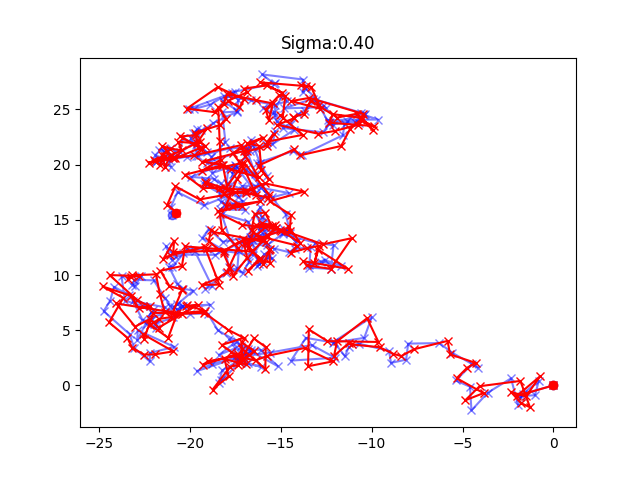
Note that the predicted line process is completely deterministic whereas the Brownian motion points has, by definition, Gaussian noise. In both cases, the actual sequence is generated by adding (additional) Gaussian noise to the predicted sequence: the -th request in the actual sequence is equal to , where are i.i.d. random variables chosen from . The value of varies, depending on the specific experiment. An example Brownian motion sequence is depicted in Fig. 3.
Set up
We use the two data sets to compare the following three algorithms:
- •
Predict refers to our algorithm, which computes the optimum solution for the predicted sequence (by using standard dynamic programming) and follows that optimum to serve actual requests.
- •
Opt is the optimum offline algorithm executed on the actual sequence. This optimum is computed by using the same dynamic programming as in the implementation of Predict.
- •
Online is state-of-the-art online randomized algorithm for page migration that achieves -approximation in expectation. This algorithm is described in Section 4.1 of [Wes94]. Since it is randomized, on each input we perform runs of Online and as the output report the average of all the runs. The standard deviation is smaller than .
For both data sets, we depict the costs of the three algorithms as a function of either or . See the text above each plots for the specification.
Results
The results for the Brownian motion data set are depicted in Fig. 4. The top two figures show the cost incurred by each algorithm for fixed values of and different values of , while the bottom two figures show the costs for fixed values of while varies. Not surprisingly, for low values of , the costs Predict and Opt are almost equal, since the predicted and the actual sequences are very close to each other. As the value of increases, their costs starts to diverge. Nevertheless, the benefit of predictions is clear, as the cost of Predict is significantly lower than the cost of Online. Interestingly, this holds even though the fraction of requests predicted exactly is very close to .
The results for the Line data set is depicted in Fig. 5. They are qualitatively similar to those for Brownian motion.


References
- [ABF93] Baruch Awerbuch, Yair Bartal, and Amos Fiat. Competitive distributed file allocation. In STOC, volume 93, pages 164–173, 1993.
- [ABF03] Baruch Awerbuch, Yair Bartal, and Amos Fiat. Competitive distributed file allocation. Information and Computation, 185(1):1–40, 2003.
- [BBM17] Marcin Bienkowski, Jaroslaw Byrka, and Marcin Mucha. Dynamic beats fixed: On phase-based algorithms for file migration. ICALP, 2017.
- [BCI97] Yair Bartal, Moses Charikar, and Piotr Indyk. On page migration and other relaxed task systems. SODA, 1997.
- [BDSV18] Maria-Florina Balcan, Travis Dick, Tuomas Sandholm, and Ellen Vitercik. Learning to branch. In International Conference on Machine Learning, pages 353–362, 2018.
- [BFK+17] Joan Boyar, Lene M Favrholdt, Christian Kudahl, Kim S Larsen, and Jesper W Mikkelsen. Online algorithms with advice: A survey. ACM Computing Surveys (CSUR), 50(2):19, 2017.
- [BFR95] Yair Bartal, Amos Fiat, and Yuval Rabani. Competitive algorithms for distributed data management. Journal of Computer and System Sciences, 51(3):341–358, 1995.
- [Bie12] Marcin Bienkowski. Migrating and replicating data in networks. Computer Science-Research and Development, 27(3):169–179, 2012.
- [BJPD17] Ashish Bora, Ajil Jalal, Eric Price, and Alexandros G Dimakis. Compressed sensing using generative models. In International Conference on Machine Learning, pages 537–546, 2017.
- [BS89] David L Black and Daniel D Sleator. Competitive algorithms for replication and migration problems. Carnegie-Mellon University. Department of Computer Science, 1989.
- [CLRW97] Marek Chrobak, Lawrence L Larmore, Nick Reingold, and Jeffery Westbrook. Page migration algorithms using work functions. Journal of Algorithms, 24(1):124–157, 1997.
- [GP19a] Sreenivas Gollapudi and Debmalya Panigrahi. Online algorithms for rent-or-buy with expert advice. In Proceedings of the 36th International Conference on Machine Learning, pages 2319–2327, 2019.
- [GP19b] Sreenivas Gollapudi and Debmalya Panigrahi. Online algorithms for rent-or-buy with expert advice. In International Conference on Machine Learning, pages 2319–2327, 2019.
- [HIKV19] Chen-Yu Hsu, Piotr Indyk, Dina Katabi, and Ali Vakilian. Learning-based frequency estimation algorithms. In International Conference on Learning Representations, 2019.
- [KBC+18] Tim Kraska, Alex Beutel, Ed H Chi, Jeffrey Dean, and Neoklis Polyzotis. The case for learned index structures. In Proceedings of the 2018 International Conference on Management of Data, pages 489–504, 2018.
- [KDZ+17] Elias Khalil, Hanjun Dai, Yuyu Zhang, Bistra Dilkina, and Le Song. Learning combinatorial optimization algorithms over graphs. In Advances in Neural Information Processing Systems, pages 6348–6358, 2017.
- [KM16] Amanj Khorramian and Akira Matsubayashi. Uniform page migration problem in euclidean space. Algorithms, 9(3):57, 2016.
- [KPS+19] Ravi Kumar, Manish Purohit, Aaron Schild, Zoya Svitkina, and Erik Vee. Semi-online bipartite matching. ITCS, 2019.
- [LLMV20] Silvio Lattanzi, Thomas Lavastida, Benjamin Moseley, and Sergei Vassilvitskii. Online scheduling via learned weights. In Proceedings of the Fourteenth Annual ACM-SIAM Symposium on Discrete Algorithms, pages 1859–1877. SIAM, 2020.
- [LRWY98] Carsten Lund, Nick Reingold, Jeffery Westbrook, and Dicky Yan. Competitive on-line algorithms for distributed data management. SIAM Journal on Computing, 28(3):1086–1111, 1998.
- [LV18] Thodoris Lykouris and Sergei Vassilvitskii. Competitive caching with machine learned advice. In International Conference on Machine Learning, pages 3302–3311, 2018.
- [Mat15] Akira Matsubayashi. A 3+ omega (1) lower bound for page migration. In 2015 Third International Symposium on Computing and Networking (CANDAR), pages 314–320. IEEE, 2015.
- [Mit18] Michael Mitzenmacher. A model for learned bloom filters and optimizing by sandwiching. In Advances in Neural Information Processing Systems, pages 464–473, 2018.
- [MMS90] Mark S Manasse, Lyle A McGeoch, and Daniel D Sleator. Competitive algorithms for server problems. Journal of Algorithms, 11(2):208–230, 1990.
- [MPB15] Ali Mousavi, Ankit B Patel, and Richard G Baraniuk. A deep learning approach to structured signal recovery. In Communication, Control, and Computing (Allerton), 2015 53rd Annual Allerton Conference on, pages 1336–1343. IEEE, 2015.
- [PSK18] Manish Purohit, Zoya Svitkina, and Ravi Kumar. Improving online algorithms via ml predictions. In Advances in Neural Information Processing Systems, pages 9661–9670, 2018.
- [Roh20] Dhruv Rohatgi. Near-optimal bounds for online caching with machine learned advice. In Proceedings of the Fourteenth Annual ACM-SIAM Symposium on Discrete Algorithms, pages 1834–1845. SIAM, 2020.
- [Unc16] Special Semester on Algorithms and Uncertainty, 2016. https://simons.berkeley.edu/programs/uncertainty2016.
- [Wes94] Jeffery Westbrook. Randomized algorithms for multiprocessor page migration. SIAM Journal on Computing, 23(5):951–965, 1994.
- [WLKC16] Jun Wang, Wei Liu, Sanjiv Kumar, and Shih-Fu Chang. Learning to hash for indexing big data - a survey. Proceedings of the IEEE, 104(1):34–57, 2016.