5^★ Knowledge Graph Embeddings with Projective Transformations

A KG is a multi-relational directed graph $\mathcal{KG}=(\mathcal{E},\mathcal{R},\mathcal{T})$ where $\mathcal{E},\mathcal{R}$ are the set of nodes (entities) and edges (relations between entities) respectively. The set $\mathcal{T}=\{(h,r,t)\}\subseteq\mathcal{E}\times\mathcal{R}\times\mathcal{E}$ contains all triples as (head, relation, tail), e.g. (smartPhone, hypernym, iPhone). In order to apply learning methods on KGs, a KGE learns vector representations of entities ($\mathcal{E}$) and relations ($\mathcal{R}$). A vector representation denoted by ($\mathbf{h,r,t}$) is learned by the model per triple $(h,r,t)$, where $\mathbf{h,t}\in\mathbb{V}^{d_{e}}$, $\mathbf{r}\in\mathbb{V}^{d_{r}}$ ($\mathbb{V}^{d}$ is a $d$-dimensional vector space). TransE (Bordes et al. 2013) considers $\mathbb{V}=\mathbb{R}$ while ComplEx (Trouillon et al. 2016) and RotatE use $\mathbb{V}=\mathbb{C}$ (complex space) and QuatE (Zhang et al. 2019) considers $\mathbb{V}=\mathbb{H}$ (quaternion space). In this paper, we choose a projective space to embed the graph i.e. $\mathbb{V}=\mathbb{CP}^{1}$ (a complex projective line which is introduced later). Most KGE models are defined via a relation-specific transformation function $g_{r}:\mathbb{V}^{d_{e}}\rightarrow\mathbb{V}^{d_{e}}$ which maps head entities to tail entities, i.e. $g_{r}(\mathbf{h})=\mathbf{t}$. On top of such a transformation function, the score function $f:\mathbb{V}^{d_{e}}\times\mathbb{V}^{d_{r}}\times\mathbb{V}^{d_{e}}\rightarrow\mathbb{R}$ is defined to measure the plausibility for triples: $f(\mathbf{h},\mathbf{r},\mathbf{t})=p(g_{r}(\mathbf{h}),\mathbf{t})$. Generally, the formulation of any score function can be either $p(g_{r}(\mathbf{h}),\mathbf{t})=-\|g_{r}(\mathbf{h})-\mathbf{t}\|$ or $p(g_{r}(\mathbf{h}),\mathbf{t})=\langle g_{r}(\mathbf{h}),\mathbf{t}\rangle$.

Projective geometry uses homogeneous coordinates which represent $N$-dimensional coordinates with $N+1$ numbers (i.e. use one additional parameter). For example, a point in 2D Cartesian coordinates, $[X,Y]$ becomes $[x,y,k]$ in homogeneous coordinates where $X=x/k,Y=y/k$ (in 1-dimensional real numbers, $[X]$ becomes $[x,y]$ where $X=x/y$). The key elements of projective geometry are as follows:

A Projective Line is a space in which a projective geometry is defined. A projective geometry requires a point at infinity to satisfy the axiom of “two parallel lines intersect in infinity”. Therefore, an extended line $\mathbb{P}^{1}(\mathbb{K})$ ($\mathbb{K}$ is a real line) is realized with $\mathbb{K}$ and a point at infinity (which topologically is a circle). More concretely, the projective line is a set $\{[x,1]\in\mathbb{P}^{1}(\mathbb{K})|x\in\mathbb{K}\}$ with an additional member $[1:0]$ denoting the point at infinity. When $\mathbb{K}=\mathbb{C}$, the projective line is complex (complex projective line denoted by $\mathbb{CP}^{1}$).

The Riemann Sphere (illustrated in Figure 9) is an extended complex plane with a point at infinity. Precisely, it is built on a plane of complex numbers wrapped around a Sphere where poles denote $0$ and $\infty$. In projective geometry, a complex projective line is a Riemann Sphere which used as a tool for projective transformations.

A Projective Transformation is the mapping of the Riemann Sphere to itself. Let $[x:y]$ be the homogeneous coordinates of a point in $\mathbb{CP}^{1}$. A projective transformation in $\mathbb{CP}^{1}$ is expressed by a matrix multiplication (Richter-Gebert 2011; Salomon 2007) as $\tau:\mathbb{CP}^{1}\rightarrow\mathbb{CP}^{1}$:

where the matrix $\Im$ must be invertible ($det(\Im)\neq 0$). By identifying $\mathbb{CP}^{1}$ with $\hat{\mathbb{C}}=\mathbb{C}\cup\{\infty\},$ a projective transformation is represented by a fractional expression through a sequence of homogenization, transformation, and dehomogenization as

where the mapping $\vartheta:\hat{\mathbb{C}}\rightarrow\hat{\mathbb{C}}$ is defined as

The resulted mapping in Equation 3 describes all Möbius transformations.

The Möbius Group is the set of all Möbius transformations which is a projective linear group $PGL(2,\mathbb{C})$, i.e. the group of all $2\times 2$ invertible matrices with the operation of matrix multiplication on a projective space. This group is the automorphism group $Aut(\hat{\mathbb{C})}$ of the Riemann Sphere $\hat{\mathbb{C}}$ or equivalently $\mathbb{CP}^{1}.$

Every Möbius transformation has at most two fixed points $\gamma_{1},\gamma_{2}$ on the Riemann Sphere obtained by solving $\vartheta(\gamma)=\gamma,$ (Richter-Gebert 2011) which gives $\gamma_{1,2}=\frac{(a-d)\pm\sqrt{\Delta}}{2c}$. Depending on the number of fixed points, Möbius transformations form parabolic or circular (one fixed point), elliptic as well as hyperbolic, and loxodromic (two fixed points) transformation functions illustrated in Figure 9. A Möbius transformation is performed on a grid by (a) a stereographic projection from complex plane to Riemann Sphere, (b) moving the Sphere, (c) stereographic projection from Sphere to plane. Each transformation has a constant $k=e^{\alpha+i\beta}$ which determines sparsity/density of the transformation. $\beta$ is an expansion factor indicating the extent to which the fixed point $\gamma_{1}$ is repulsive ($\gamma_{2}$ is attractive). $\alpha$ is a rotation factor, determining the degree to which a transformation rotates the plane counter-clockwise around $\gamma_{1}$ (clockwise around $\gamma_{2}).$

Embedding on a Complex Projective Line Given a triple $(h,r,t)$, the head and tail entities $h,t\in\mathcal{E}$ are embedded into a $d$ dimensional complex projective line i.e. $\mathbf{h,t}\in\mathbb{CP}^{d}$. A relation $r\in\mathcal{R}$ is embedded into a $d$ dimensional vector $\mathbf{r}$ where each element is a $2\times 2$ matrix. $\mathbf{r}$ contains four complex vectors $\mathbf{r_{a}},\mathbf{r_{b}},\mathbf{r_{c}}$ and $\mathbf{r_{d}}\in\mathbb{C}^{d}$. With $\mathbf{r}_{ai},\mathbf{r}_{bi},\mathbf{r}_{ci},\mathbf{r}_{di},\mathbf{h}_{i},\mathbf{t}_{i}$, we refer to the $i$th element of $\mathbf{r}_{a},\mathbf{r}_{b},\mathbf{r}_{c},\mathbf{r}_{d},\mathbf{h},\mathbf{t}$ respectively.

Relation-specific Transformation Based on preliminaries a projective transformation on a complex projective line has an equivalent transformation on the Riemann Sphere. Therefore, we use both of these perspectives in our model formulation.

Möbius Representation of Transformation: We use a relation-specific Möbius transformation to map the head entity ($\mathbf{h}_{ri}$) from a source to a target complex plane ($\hat{\mathbb{C}}$). The transformation is performed using stereographic projection and transformation ($\vartheta$) on/from the Riemann Sphere. To do so, we compute $\mathbf{h}_{ri}$ to specify the element-wise transformation:

This results in the relation-specific transformed head entity $\mathbf{h}_{r}=[\mathbf{h}_{r1},\ldots,\mathbf{h}_{rd}].$

Projective Representation of Transformation: Using homogeneous coordinates, we can also represent Equation 15 as a projective transformation:

where $\doteq$ shows dehomogenization, $\Im_{ri}=\begin{bmatrix}\mathbf{r}_{ai}\,&\mathbf{r}_{bi}\\ \mathbf{r}_{ci}\,&\mathbf{r}_{di}\end{bmatrix}$ and $\det{\Im_{ri}}\neq 0$ i.e. $\Im_{ri}s$ are invertible. The matrix representation of Equation 12 is $\mathbf{h}_{r}=\mathbf{R_{r}}[\mathbf{h}:\mathbf{1}],$ where $\mathbf{R_{r}}=diag(\Im_{r1}\ldots,\Im_{rd})$ and $\mathbf{1}$ is a vector with all the elements being 1.

Score Function The correctness of triples in a KG is the similarity $\langle\mathbf{h}_{r},\mathbf{t}\rangle$ between the relation-specific transformed head $\mathbf{h}_{r}$ and tail $\mathbf{t}$. The model aims to minimize the angle between $\mathbf{h}_{r}$ and tail $\mathbf{t}$, i.e. their product ($\langle\mathbf{h}_{r},\mathbf{t}\rangle$) is maximized for positive triples. For sampled negative triples, it is conversely minimized. Overall, the score function for $5^{\bigstar}$E is

where $Re(x)$ is the real part of the complex number $x$.

We first show that $5^{\bigstar}$E covers the five transformations. We then discuss the capability of $5^{\bigstar}$E in preserving graph structures. We also prove $5^{\bigstar}$E is fully expressive and subsumes various state-of-the-art KGE models.

Möbius – Composition of Transformations The Möbius transformation in Equation 15 is a composition of a series of five subsequent transformations $\vartheta_{1},\vartheta_{2}\text{(two transformations in one)},\vartheta_{3}$ and $\vartheta_{4}$ as shown in (Kisil 2012): $\mathbf{h}_{ri}=\vartheta(\mathbf{h}_{i},\mathbf{r}_{i})=\vartheta_{4}\circ\vartheta_{3}\circ\vartheta_{2}\circ\vartheta_{1}(\mathbf{h}_{i},\mathbf{r}_{i})$, where $\vartheta_{1}(\mathbf{x},\mathbf{r}_{i})=\mathbf{x}+\frac{\mathbf{r}_{di}}{\mathbf{r}_{ci}}$ (translation by $\frac{\mathbf{r}_{di}}{\mathbf{r}_{ci}}$), $\vartheta_{2}(\mathbf{x})=\frac{1}{\mathbf{x}}$ (inversion and reflection w.r.t. real axis), $\vartheta_{3}(\mathbf{x},\mathbf{r}_{i})=\frac{\mathbf{r}_{bi}\mathbf{r}_{ci}-\mathbf{r}_{ai}\mathbf{r}_{di}}{\mathbf{r}_{ci}^{2}}\mathbf{x}$ (homothety and rotation) and $\vartheta_{4}(\mathbf{x},\mathbf{r}_{i})=\mathbf{x}+\frac{\mathbf{r}_{ai}}{\mathbf{r}_{ci}}$ (translation by $\frac{\mathbf{r}_{ai}}{\mathbf{r}_{ci}})$. This shows that $5^{\bigstar}$E is capable of performing 5 transformations simultaneously.

Capturing Structures in a Neighborhood 5^★E inherits various important properties of projective transformation as well as Möbius transformations. Because the projective linear group $PGL(2,\mathbb{C})$ is isomorphic to the Möbius group, i.e., $PGL(2,\mathbb{C})\cong Aut(\mathbb{\hat{C}})$ (Kisil 2012), the properties which are mentioned for Equation 12 are also valid for Equation 15. We investigate the inherited properties of 5^★E on clustering similar nodes of a neighborhood and Capturing Sub-graph Structures.

Clustering. The similarity of nodes in a KG is local, i.e. nodes within a close neighborhood are more likely to be semantically similar (Faerman et al. 2018; Hamilton, Ying, and Leskovec 2017) than nodes at a higher distance. A projective transformation is a bijective conformal mapping, i.e. it preserves angle locally but not necessarily the length. It also preserves orientation after mapping (Kisil 2012). Therefore, 5^★E is capable of capturing similarity by preserving angle locally via a relation-specific transformation.

Furthermore, the map $\pi:GL(2,\mathbb{C})\rightarrow Aut(\mathbb{\hat{C}})$ is a group homomorphism, where $GL(2,\mathbb{C)}$ is a generalized linear group, which transfers the matrix $\Im$ into a Möbius transformation $\vartheta$. If $\det{\Im}=1,$ then $\pi:SL(2,\mathbb{C})\rightarrow Aut(\mathbb{\hat{C}})$ becomes limited to only perform a mapping from the special linear group $SL(2,\mathbb{C})$ to a Möbius group that preserves volume and orientation.

In the context of KGs, after a relation-specific transformation (Equation 12 or equivalently Equation 15) of nodes in the head position to nodes in tail position, the relative distance of nodes can be preserved. From this ability, we expect that 5^★E is able to propagate the structural similarity from one group of nodes to another.

Capturing Sub-graph Structures. Going beyond $SL(2,\mathbb{C})$ by changing the determinant to $\det\Im\neq 1$, the volume and orientation of the graph sub-structures are changed after transformation. Therefore, 5^★E is more flexible than current KGEs as those are not able to change volume and orientation of subgraphs. This is visible in Figure 1 when the graph includes a group of nodes in a path structure besides another group of nodes with a loop structure. In the vector space, other KGEs encounter a problem in preserving this type of graph structure due to the limited transformation abilities (not supporting inversion and reflection), whereas they work fine for homogeneous structures (e.g. only lines or only circles). In contrast to this, 5^★E is capable of transforming heterogeneous structures due to the characteristics of a projective transformation (Kisil 2012).

Subsumption of Other Models We show that 5^★E subsumes other models and inherits their favorable characteristics in learning various graph patterns.

Inference of Patterns For relations which exhibit patterns in the form of $\textit{premise}\rightarrow\textit{conclusion}$, where premise can be a conjunction of several triples, a model is said to be able to infer those if the implication holds for the score function, i.e. if the score of all triples in the premise is positive then the score for the conclusion must be positive. 5^★E is able to infer reflexive, symmetric, inverse relation patterns as well as composition.

TransE only infers composition and inverse patterns. RotatE is capable of inferring more patterns but is not fully expressive. ComplEx infers these patterns and is fully expressive. However, it has less flexibility than our model in learning complex structures due to using only rotation and homothety. Therefore, it is only capable of preserving homogeneous structures (see Figure 5).

Here, we demonstrate an example for the cases presented in Figure 1 in the main body of the paper. We choose path/loop relation to build up our example. Assume that, we have a set of 10 different nodes which are positioned as a path ($h_{i}$ where $i\dots 10$) of a specific relation (e.g. hypernym). A different set of another 10 nodes ($t_{i}$ where $i\dots 10$) are connected through a relation (e.g. similar_to) in a loop structure. Our assumption is that the path structure is positioned beside a loop. The nodes in the head position are collected (e.g. through the also-see relation) to the ones in the loop position. In Figure 8, the given ranking by each embedding model for each triple is shown. Low number means a better ranking for higher plausibility of each triple, and high ranking means the chance of triple incorrectness is high. Column one shows all the possible triples which are involved in these three relations. We consider bi-directional ranking as “right hand side ranking”(RHS) and “left hand side ranking”(LHS).

The highlights to be noted are that:

• •

  In order to preserve the shape of the loop, the triple $(t_{10},\,similar-to,\,t_{1})$ should be ranked as low as possible. The problem occurs when a model gives a high rank to this triple. If this happens, the shape of the loop is transferred (wrongly) to a path.

• •

  In order to preserve the shape of the path, the $(h_{10},\,similar-to,\,h_{1})$ triple should be ranked as high as possible. The problem occurs when a model gives a low rank to this triple. If this happens, the shape of the path is transferred (wrongly) to a loop.

A perfect model should specifically learn $(t_{10},\,similar-to,\,t_{1})$ as positive (rank low) in order to preserve the loop. Moreover, the model should learn $(h_{10},\,similar-to,\,h_{1})$ as a negative triple with a high rank which means the path shape is preserved.

For $(t_{10},\,similar-to,\,t_{1})$ triple which is expected to be ranked very low by a good KGE model, $5^{\bigstar}$E ranks this triple as low as possible (2 both for LHS and RHS), without problematically affecting the ranking of $(h_{10},\,similar-to,\,h_{1})$ triple (ranked high as 19, 18 ). This concludes that the shape of loop and path are preserved by $5^{\bigstar}$E. However, other models completely miss-preserve the head triple of $(h_{10},\,similar-to,\,h_{1})$ when they take a low rank for $(t_{10},\,similar-to,\,t_{1})$. This is more visible for QuatE and RotatE. RotatE learns $(t_{10},\,similar-to,\,t_{1})$ with lowest rank (1), however it also ranks $(h_{10},\,similar-to,\,h_{1})$ with 1. Relatively similar behaviours is observed from QuatE. This concludes that the shape of loop is preserved by RotatE and QuatE, however it was with the cost of (wrongly) transferring path to loop as well. For TransE, a relatively high ranking is assigned to $(h_{10},\,similar-to,\,h_{1})$ triple (which means the model expects this triple to be incorrect) and preserves the path, however this causes a high rank for $(t_{10},\,similar-to,\,t_{1})$ as well. We see in that by using the ComplEx model, it shows a similar behaviour to TransE model. This concludes that the shape of path is preserved, however the loop part is also transferred to a path shape. This observation in connection to Figure 1 clarifies the difficulty of other KGE models when different motifs come close in subgraphs of a KG. Our proposed model has the potential to correctly preserve each structure separately. This power comes from the possible transformations covered in projective geometry, illustrated in Figure 9. In Table 4, the theoretical description and the validity conditions of each transformation is discussed. All transformations in each group form a subgroup which is isomorphic to the group of all matrices mentioned in the row Iso. Note that $tr$ in the table denotes the trance of a matrix.

As mentioned in the main paper, the RotatE model is not able to preserve a loop structure connected with a path from the graph representation in the vector space. To show this, without loss of generality, we investigate the example given in Figure one with a concrete scenario. Let us consider three entities ($h_{1},h_{2},h_{3}$) connected by the relation $r_{1}$ in a path structure i.e. $(h_{1},r_{1},h_{2}),(h_{2},r_{1},h_{3})$, and three other entities $(t_{1},t_{2},t_{3})$ connected by relation $r_{3}$ in a loop structure i.e. $(t_{1},r_{1},t_{2}),(t_{2},r_{1},t_{3}),(t_{3},r_{1},t_{1})$. RotatE encodes path as

and loop as

Additionally, entities of the path structure are connected to the entities of the loop structure i.e. $(h_{1},r_{2},t_{1}),(h_{2},r_{2},t_{2}),(h_{3},r_{2},t_{3})$, which are encoded by RotatE as

Note that the representation of relations between entities is actually a rotation in complex space when using RotatE model i.e. $\mathbf{r}=e^{i\theta}$.

After combining Equation 7 and 8, we have

After replacing $\mathbf{t}_{2}$ by $\mathbf{h}_{2}\circ\mathbf{r}_{2}$ (according to equation 9) in equation 10, we have

Comparing equation 11 and 7, we have $\mathbf{r}_{1}=\mathbf{r}_{3}.$ Therefore, $\mathbf{h}_{3}\circ\mathbf{r_{3}}\approx\mathbf{h}_{1}$ and $\mathbf{h}_{3}\circ\mathbf{r_{1}}\neq\mathbf{h}_{1}$ should be held simultaneously which is in contradiction with $\mathbf{r}_{1}=\mathbf{r}_{3}.$ Based on the above-mentioned results, RotatE cannot encode loop connected with path in the vector space and either loop becomes path or path becomes loop. Similarly, we prove that other models such as QuatE (rotation in Quaternion space) and ComplEx (rotation in complex space together with homothety) also face issues when transforming a path beside a loop structure. In Table 3, we show the capability of KGEs in preserving different transformations. Correctly learning of one of these two triples, scarifies the other.

As mentioned in the paper, our model uses bijective conformal mapping in the projective geometry which consequently preserves angle locally but not necessarily the length of motifs. Such characteristic is consistent with the nature of KGs where similarity of nodes in the graph is local i.e. nodes within a close neighborhood are more likely to be semantically similar than nodes at a higher distance. Figures 10, 11 and 12 show the clustering results of each model of QuatE, ComplEx and 5$\bigstar$E. According to this visualizations, 5$\bigstar$E puts entities of the same type more closer (lower variance) than other competitors. Moreover, the distance between center of clusters in 5$\bigstar$E is bigger than other models. Therefore, it is visible that 5$\bigstar$E provides a more accurate clustering than other competitors.

In Table 5, the results of experimenting 5^★E on FB15K and WN18 are compared to other models. In WN18, 5^★E outperforms all the models in all the metrics expect Hits@10 where 0.96 is achieved by RotatE, TuckEr, QuatE, and ConvE as well as 5^★E. On the FB15k dataset, we observe that 5^★E outperforms TransE, RotatE, TuckEr, ComplEx, SimplE, and ConvE on FB15K. 5^★E and QuatE achieve a very competitive results in most of the cases. In MRR, our model performs slightly better, and in Hits@1, QuatE is better.

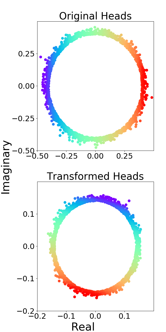
One of the main advantage of 5^★E lies in its ability to map a line to a circle after a relation-specific transformation of the head. This means that for a given relation, e.g., hypernym, if the embeddings of the entities in the head position form a line, each of the transformed heads are either forming a line or a circle. Consequently, according to the formula $\mathbf{h}_{ri}=g_{r}(\mathbf{h}_{i})=\bar{\mathbf{t}}_{i},i=1,\ldots,d$, the conjugated tails should also represent a shape which is close to the corresponding transformed head. In this way, 5^★E captures different structural motifs of different groups of nodes. The Figures 14 and 13 illustrate the state of each relation in different dimensions with regard to their original head, transformed head, and conjugated tail. Figure 14 depicts transformations in four different dimensions for the hypernym relation where the line shows head entities which are located on a line and the transformed heads start to develop in the shape of a circle. Given a fixed relation $r$ (e.g., hypernym), the similarity between all the transformed heads (which form a line or a circle) and the conjugated tails (similarly form a line or a circle) shows that the triples are considered positive in the vector space i.e.  $g_{r}(\mathbf{h}_{ij})=\bar{\mathbf{t}}_{ij},i=1,\ldots,d,j=1,\ldots,n$ where $n$ refers to the number of entities in the head/tail position. $h_{ij}$ refers to the $i$th dimension of embeddings for $j$th head entity. In one dimension, all the heads in Figure 13 form a line which are after transformation form a circle. Note that in each dimension ($i$th dimension), 5^★E learns different transformation functions. Each entity in head is shown as a point Therefore, by taking different dimensions, the shape of the transformations changes per relation.

The two relations hyponym and hypernym are inverse of each other. Therefore, we have $\Im_{\textit{Hypernym}}=\bar{\Im}^{-1}_{\textit{Hyponym}}.$ As these representing matrices ($\Im$) are normalized, their determinant is equal to one. Consequently, we have $tr(\Im_{\textit{Hypernym}})=tr(\bar{\Im}^{-1}_{\textit{Hyponym}})$ when the learned transformation function is elliptic. We conclude that for a pair of inverse relations, the learned transformation functions are in the same category (elliptic) for the $i$th element of the relation embedding. Figure 15, sub-figure (a) and (b) illustrate that the learned functions fall into the elliptic category for the same embedding dimension ($i=12$) of hyponym and hypernym. The difference between the embeddings for this pair of inverse relations is their rotation. The same pattern is notable for hasPart and partOf relations in sub-figure (c) and (d) on $i=39$.

Construction Steps of Transformations

In Figure 16 we show the learned 5^★E embeddings for hasType relations in different epochs ranging from 0 to 49 (the stabilized epoch for this relation). The figure illustrates the gradual development of the Möbious shape over different epochs.

• •

  Evaluation Metrics and Statistics of Standard Benchmarks FB15K is a standard benchmark created from the original FreeBase KG (Bollacker et al. 2008). FB15K-237 (Toutanova and Chen 2015) is a sub-version of FB15K in which the inverse relations have been removed. WN18 (Bordes et al. 2013) is a lexical database with hierarchical collection for the English language that was derived from the original WordNet dataset (Miller 1995). The main relation patterns in this dataset are symmetry antisymmetry and inversion. WN18RR is a sub-version of WN18 for which the inverse relations are omitted. We also considered four different versions of the NELL dataset in our evaluations. In Table 6, we represent the statistics of each corresponding detest.

• •

  Hyperparameter Search Generally, the range of embedding dimensions were fixed to {100, 500 } with learning rates of {0.01, 0.05, 0.1 }, except for the versions of NELL datasets, where d = 200 was used. This was done to show the effectiveness of the model in different dimensions. The considered batch sizes for all datasets are {100, 500, 1000, 2000 }. Regularization coefficients are tested among {0.01, 0.05, 0.1, 0.5 }. For all the required values in our evaluation tables, which were not reported in the original papers, we trained the models and reported our findings. To train models on NELL-995-h25, NELL-995-h50, NELL-995-h75 and NELL-995-h100, we proceeded as follows: First, the NELL-995-h25 dataset was used to find the best hyperparameter setting among the aforementioned hyperparameter settings. After the best setting is found per model, the same hyperparameters for each model are applied to NELL-995-h50, NELL-995-h75 and NELL-995-h100. The same fixed hyperparameters per model are then also used when training a NELL-995-h25 model with a different embedding dimension.

In this part, we prove that 5^★E subsumes five popular KGE models namely DistMult, ComplEx, pRotatE, RotatE and TransE. Here, we provide proofs for the following items:
(a) $5^{\bigstar}$E subsumes DistMult with its original score function $f(h,r,t)=Re(\langle\mathbf{h}_{r},\bar{\mathbf{t}}\rangle),$ where

Note that here we use homogeneous coordinates. With the symbol $\doteq$, we mean that the left hand side of Equation 12 (i.e. $g_{r}(\mathbf{h}_{i})$) equals the results of the right hand side after dehomogenization.

(b) $5^{\bigstar}$E subsumes pRotatE with its original score function $f(h,r,t)=Re(\langle\mathbf{h}_{r},\bar{\mathbf{t}}\rangle)$.

(c) $5^{\bigstar}$E subsumes ComplEx with its original score function $f(h,r,t)=Re(\langle\mathbf{h}_{r},\bar{\mathbf{t}}\rangle)$.

(d) $5^{\bigstar}$E subsumes RotatE with score function $f(h,r,t)=-\|\mathbf{h}_{r}-\mathbf{t}\|$ (changed inner product to distance).

(e) $5^{\bigstar}$E subsumes TransE with score function $f(h,r,t)=-\|\mathbf{h}_{r}-\mathbf{t}\|$ (changed inner product to distance).

References

- Balazevic, Allen, and Hospedales (2019a) Balazevic, I.; Allen, C.; and Hospedales, T. 2019a. Multi-relational Poincaré graph embeddings. In Advances in Neural Information Processing Systems, 4465–4475.
- Balazevic, Allen, and Hospedales (2019b) Balazevic, I.; Allen, C.; and Hospedales, T. 2019b. TuckER: Tensor Factorization for Knowledge Graph Completion. In EMNLP-IJCNLP Conference, 5188–5197.
- Bollacker et al. (2008) Bollacker, K.; Evans, C.; Paritosh, P.; Sturge, T.; and Taylor, J. 2008. Freebase: a collaboratively created graph database for structuring human knowledge 1247–1250.
- Bordes et al. (2013) Bordes, A.; Usunier, N.; Garcia-Duran, A.; Weston, J.; and Yakhnenko, O. 2013. Translating embeddings for modeling multi-relational data. In Advances in neural information processing systems, 2787–2795.
- Chami et al. (2020) Chami, I.; Wolf, A.; Juan, D.-C.; Sala, F.; Ravi, S.; and Ré, C. 2020. Low-Dimensional Hyperbolic Knowledge Graph Embeddings. In Proceedings of the 58th Annual Meeting of the Association for Computational Linguistics, 6901–6914.
- Dettmers et al. (2018) Dettmers, T.; Minervini, P.; Stenetorp, P.; and Riedel, S. 2018. Convolutional 2d knowledge graph embeddings. In Thirty-Second AAAI Conference.
- Faerman et al. (2018) Faerman, E.; Borutta, F.; Fountoulakis, K.; and Mahoney, M. W. 2018. Lasagne: Locality and structure aware graph node embedding. In International Conference on Web Intelligence (WI), 246–253. IEEE.
- Hamilton, Ying, and Leskovec (2017) Hamilton, W. L.; Ying, R.; and Leskovec, J. 2017. Representation learning on graphs: Methods and applications. arXiv preprint arXiv:1709.05584 .
- Ji et al. (2015) Ji, G.; He, S.; Xu, L.; Liu, K.; and Zhao, J. 2015. Knowledge graph embedding via dynamic mapping matrix. In Proceedings of the 53rd Annual Meeting of the Association for Computational Linguistics and the 7th International Joint Conference on Natural Language Processing (Volume 1: Long Papers), 687–696.
- Ji et al. (2016) Ji, G.; Liu, K.; He, S.; and Zhao, J. 2016. Knowledge Graph Completion with Adaptive Sparse Transfer Matrix. 985–991.
- Ji et al. (2020) Ji, S.; Pan, S.; Cambria, E.; Marttinen, P.; and Yu, P. S. 2020. A survey on knowledge graphs: Representation, acquisition and applications. arXiv preprint arXiv:2002.00388 .
- Kazemi and Poole (2018) Kazemi, S. M.; and Poole, D. 2018. Simple embedding for link prediction in knowledge graphs. In Advances in neural information processing systems, 4284–4295.
- Kisil (2012) Kisil, V. V. 2012. Geometry of Möbius Transformations: Elliptic, Parabolic and Hyperbolic Actions of SL2 [real Number]. World Scientific.
- Lacroix, Usunier, and Obozinski (2018) Lacroix, T.; Usunier, N.; and Obozinski, G. 2018. Canonical Tensor Decomposition for Knowledge Base Completion. In International Conference on Machine Learning (ICML), 2863–2872.
- Lin et al. (2015) Lin, Y.; Liu, Z.; Sun, M.; Liu, Y.; and Zhu, X. 2015. Learning entity and relation embeddings for knowledge graph completion. In Twenty-ninth AAAI conference on artificial intelligence.
- Miller (1995) Miller, G. A. 1995. WordNet: a lexical database for English. Communications of the ACM 38(11): 39–41.
- Moon, Jones, and Samatova (2017) Moon, C.; Jones, P.; and Samatova, N. F. 2017. Learning entity type embeddings for knowledge graph completion. In Proceedings of the 2017 ACM on conference on information and knowledge management, 2215–2218.
- Nickel and Kiela (2018) Nickel, M.; and Kiela, D. 2018. Learning Continuous Hierarchies in the Lorentz Model of Hyperbolic Geometry. volume 80 of Proceedings of Machine Learning Research, 3779–3788. PMLR.
- Nickel, Tresp, and Kriegel (2011) Nickel, M.; Tresp, V.; and Kriegel, H.-P. 2011. A Three-Way Model for Collective Learning on Multi-Relational Data. 11: 809–816.
- Richter-Gebert (2011) Richter-Gebert, J. 2011. Perspectives on projective geometry: A guided tour through real and complex geometry. Springer Science & Business Media.
- Salomon (2007) Salomon, D. 2007. Transformations and projections in computer graphics. Springer Science & Business Media.
- Socher et al. (2013) Socher, R.; Chen, D.; Manning, C. D.; and Ng, A. 2013. Reasoning with neural tensor networks for knowledge base completion 926–934.
- Sun et al. (2019) Sun, Z.; Deng, Z.-H.; Nie, J.-Y.; and Tang, J. 2019. Rotate: Knowledge graph embedding by relational rotation in complex space. arXiv preprint arXiv:1902.10197 .
- Tim Hutton (2020) Tim Hutton. 2020. Mobius Transforms. https://github.com/timhutton/mobius-transforms. Online; accessed 15 December 2020.
- Toutanova and Chen (2015) Toutanova, K.; and Chen, D. 2015. Observed versus latent features for knowledge base and text inference. In Proceedings of the 3rd Workshop on Continuous Vector Space Models and their Compositionality, 57–66.
- Trouillon et al. (2016) Trouillon, T.; Welbl, J.; Riedel, S.; Gaussier, É.; and Bouchard, G. 2016. Complex embeddings for simple link prediction. In International Conference on Machine Learning, 2071–2080.
- Wang, Gemulla, and Li (2018) Wang, Y.; Gemulla, R.; and Li, H. 2018. On multi-relational link prediction with bilinear models. In Thirty-Second AAAI Conference on Artificial Intelligence.
- Wang et al. (2014) Wang, Z.; Zhang, J.; Feng, J.; and Chen, Z. 2014. Knowledge graph embedding by translating on hyperplanes. In Twenty-Eighth AAAI conference on artificial intelligence.
- Weber and Nickel (2018) Weber, M.; and Nickel, M. 2018. Curvature and Representation Learning: Identifying Embedding Spaces for Relational Data. NeurIPS Relational Representation Learning .
- Xiong, Hoang, and Wang (2017) Xiong, W.; Hoang, T.; and Wang, W. Y. 2017. DeepPath: A Reinforcement Learning Method for Knowledge Graph Reasoning. In EMNLP Conference, 564–573.
- Yang et al. (2015) Yang, B.; Yih, W.-t.; He, X.; Gao, J.; and Deng, L. 2015. Embedding entities and relations for learning and inference in knowledge bases. In Conference on Learning Representations (ICLR).
- Zhang et al. (2019) Zhang, S.; Tay, Y.; Yao, L.; and Liu, Q. 2019. Quaternion knowledge graph embeddings. In Advances in Neural Information Processing Systems, 2731–2741.
Appendix
Capturing Path/loop