An algorithmic Introduction to Clustering

Let $x\in\mathbb{R}^{d}$ be a $d$-dimensional random vector. A Gaussian distribution (also known as Normal distribution) with mean vector $\mu\in\mathbb{R}^{d}$ and covariance matrix $\Sigma\in\mathbb{R}^{d\times d}$ can be written in the form:

where $|\Sigma|$ denotes the determinant of $\Sigma$ and $x^{T}$ is the transpose of vector $x$.

Given a dataset $X$ composed by $n$ i.i.d. data points $x_{1},x_{2},...,x_{n}$, where $\forall i,x_{i}\in\mathbb{R}^{d}$, we can use a Gaussian Distribution as a model to fit this dataset. A common criterion for fitting the parameters $\mu$ and $\Sigma$ of the Gaussian distribution given an observed dataset is to find the values that maximize the likelihood function:

This procedure is known as Maximum Likelihood Estimation (MLE). Given the form of the Gaussian distribution, it is more convenient to maximize the $\log$ of the likelihood function (maximizing this is equivalent because the logarithmic function is a monotonically increasing function). Taking $\log$ on both sides

Maximizing with respect to $\mu$ (i.e., taking the derivative of $\log p(X|\mu,\Sigma)$ w.r.t. $\mu$ and equalizing to zero), we obtain

Similarly, maximizing w.r.t. $\Sigma$

As we can see, fitting one Gaussian distribution to a dataset $X$ using maximum likelihood is a simple procedure, as shown in algorithm 1. The complexity of this algorithm is $O(nd^{2})$, due the computation of matrix $\Sigma_{MLE}$.

Figure 2(a) shows a dataset with 500 points in two dimensions. Figure 2(b) shows the same dataset and the learned configuration for the Gaussian model. The mean and the three standard-deviation contour for this model are shown as a red point and a red ellipse, respectively.

After fitting the model to the data distribution, we can sample from it and compare how a set of samples looks with respect to the original dataset. Figure 3 shows a set of 500 points sampled from the data (in red) along with the 500 original data points (in blue). We can observe a couple of things: the space covered by the sampled points is similar to the space covered by the original data points, and any of the sampled points are "close" to at least one of the original data points. Despite not being a quantitative measure, figure 3 allow us to form an intuition of how well the model fitted the data for this two dimensional dataset.

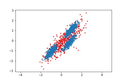
As we can imagine, there exists datasets for which one Gaussian distribution doesn’t offer the flexibility to fit the data points in the dataset to analize. Figure 4(a) shows a dataset with 1500 points in two dimensions. We will denote this dataset as $X_{1500}$. Figure 4(b) shows the dataset $X_{1500}$ and the learned configuration for one Gaussian model. Like in the previous example, the three standard-deviation contour is shown as a red ellipse. However, in this case, we can observe how the model doesn’t capture the data distribution as well as in the previous example. Specifically, sampling from the learned distribution generates points which are "far" from any of the original data points, as shown in figure 4(c). Also, we can observe how the sampled points cover parts of the space not covered by the original data points.

One way to add more flexibility to our model is to use instead a Mixture of Gaussians. A superposition of $k$ Gaussian densities of the form:

is called a mixture of Gaussians. Each Gaussian density $\mathcal{N}(x|\mu_{c},\Sigma_{c})$ is called a component of the mixture and has its own mean $\mu_{c}$ and covariance matrix $\Sigma_{c}$. The parameters $\pi_{c}\in\mathbb{R}$ are called mixing coefficients, and have two important properties:

We can view the mixing coefficients $\pi_{c}$ as the prior probability $p(c)$ of picking the $c$-th component. Similarly, we can view the Gaussian densities $\mathcal{N}(x|\mu_{c},\Sigma_{c})$ as the probability of $x$ conditioned on $c$, $p(x|c)$ (i.e., the likelihood of point $x$ given the $c$-th component). Using this notation, we can express equation (6) as:

From here, we can see that we can compute the posterior probabilities $p(c|x)$ using Bayes’ theorem:

Following the notation in [1], we denote the variables $\lambda_{i,c}$ as "responsibilities", and we will use the following notation: $\boldsymbol{\pi}\equiv\{\pi_{1},...,\pi_{k}\}$, $\boldsymbol{\mu}\equiv\{\mu_{1},...,\mu_{k}\}$ and $\boldsymbol{\Sigma}\equiv\{\Sigma_{1},...,\Sigma_{k}\}$. These responsibilities $\lambda_{i,c}$ can be interpreted as a measure of how much the point $x_{i}$ "belongs" to the $c$-th component, given the current estimates $\boldsymbol{\mu}$ and $\boldsymbol{\Sigma}$. Similar to what we did with one Gaussian distribution, we can try to fit the parameters of this model given an observed dataset $X$ using maximum likelihood. Using the i.i.d. assumption and equation (6) we have

The situation now is much more complex than with a single Gaussian, due to the presence of the summation inside the logarithm. As a result, the maximum likelihood solution for the parameters of the GMM no longer has a closed-form analytical solution. Maximizing equation (11) with respect to $\mu_{c}$, we obtain

where $n_{c}=\sum^{n}_{i=1}\lambda_{i,c}$. Similarly, maximizing equation (11) w.r.t. $\Sigma_{c}$

Finally, we need to maximize equation (11) w.r.t. $\pi_{c}$. However, in this case we need to take into acount the constraints (7) and (8). This can be achieved using Lagrange multipliers, getting as result

Despite looking as closed-form solutions, equations (12),(13) and (14) are not such, because all of them are functions of the responsibilities $\lambda_{i,c}$. However, these responsibilities depends on $\boldsymbol{\pi},\boldsymbol{\mu},\boldsymbol{\Sigma}$ in a complex way, as we can see from equation (10).

However, the last three equations suggest a simple iterative algorithm to find a solution to the GMM maximum likelihood problem:

• •

  First, we choose some initial values for the means $\mu_{c}$, matrices $\Sigma_{c}$ and mixing coefficients $\pi_{c}$

• •

  Then, we alternate between the following two updates, that we shall call the E step (from Expectation) and M step (from Maximization):

  • –

    In the E step, we use the current values of $\mu_{c}$, $\Sigma_{c}$ and $\pi_{c}$ to compute the responsibilities $\lambda_{i,c}$ using equation (10)

  • –

    Then, we use these $\lambda_{i,c}$ in the M step to re-estimate the values of $\mu_{c}$, $\Sigma_{c}$ and $\pi_{c}$ using equations (12),(13) and (14), respectively

It is important to highlight that when computing the update for $\Sigma^{new}_{c}$, we use the updated values of $\mu^{new}_{c}$. The algorithm iterates until a convergence criteria is met. In practice, the algorithm is deemed to have converged when the change in the log likelihood function , or alternatively in the parameters, falls below some threshold.

This iterative procedure using the E step and M step is an instance of a more general algorithm called Expectation-Maximization algorithm. The EM algorithm is an iterative procedure to find maximum likelihood solutions for models having latent variables. It should be emphasized that commonly, the log likelihood function has multiple local maxima, and that the EM algorithm is not guaranteed to find the global maxima. The EM algorithm for Gaussian Mixtures models (EM-GMM algorithm) is shown in algorithm 2.

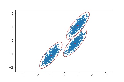
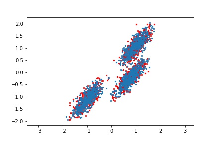
EM-GMM is the first clustering algorithm presented in this document: it takes a collection $X$ of $n$ points in a $d$ dimensional space and group them into $k$ different clusters $\Gamma_{1},\Gamma_{2},...,\Gamma_{k}$ using a mixture of Gaussians as a model. Every Gaussian distribution models a cluster $\Gamma_{c}$. Figure 5(a) shows how a GMM model with three components is able to fit the previous dataset more tightly than the one-Gaussian model. Also, sampling from the GMM model generates points which are more similar to points in the original dataset, as shown in figure 5(b). We can also observe how the space covered by the sampled points is now more similar to the space covered by the original data points.

At every iteration, the two updates more computationally intensive are the update of $\lambda_{i,c}$ in E step and the update of the matrices $\Sigma_{c}$ in the M step.

Specifically, at every iteration, the E step requires the evaluation of $nk$ Gaussian distributions, which involves the computation (for every cluster $\Gamma_{c}$) of the determinant and the inverse of a matrix of size $d\times d$, both with complexity $O(d^{2.807})$ for practical purposes (using Strassen algorithm for matrix multiplication, however there are algorithms asymptotically faster). Also, for every $x_{i}$, we need to compute a quadratic form w.r.t. every cluster $\Gamma_{c}$, with complexity $O(d^{2})$, therefore resulting in an overall complexity of $O(nd^{2}k)$. Therefore, the overall complexity for E step at every iteration is $O(nd^{2}k+d^{2.807}k)$.

Similarly, the update of any of the matrices $\Sigma_{c}$ requires the computation and addition of $n$ matrices of size $d\times d$, with complexity $O(nd^{2})$, therefore resulting in an overall complexity of $O(nd^{2}k)$ for M step at every iteration.

Therefore, the complexity of the EM-GMM algorithm is $O(nd^{2}kT+d^{2.807}kT)$, where $T$ denotes the number of iterations. This complexity and other important properties of the EM-GMM algorithm are summarized in table 1.

A GMM returns what is called a soft assignment for every data point $x_{i}$: instead of assigning it to a specific cluster $\Gamma_{c}$, it returns a "responsibility" $\lambda_{i,c}$, expressing how "responsible" is cluster $\Gamma_{c}$ for data point $x_{i}$. The set of $\lambda_{i,c}$ for a specific point $x_{i}$ forms a distribution over the clusters $\Gamma_{1},\Gamma_{2},...,\Gamma_{k}$. On the other hand, a hard assignment is an assignment where every point $x_{i}$ is assigned to exactly one cluster $\Gamma_{c}$.

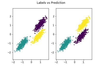
One simple way to turn the soft assignment returned by a GMM into a hard assignment is to assign point $x_{i}$ to the cluster $\Gamma_{c}$ with larger responsability $\lambda_{i,c}$. Using this rounding method, we can observe in figure 6 how the clusters found by the GMM model (right side) compare to the labels from the $X_{1500}$ dataset (left side).

Consider a GMM model with all covariance matrices equal to the identity matrix $I$ times a variance parameter $\epsilon$, i.e., $\Sigma_{c}=\epsilon I$ $\forall c$. Then, for point $x$ and cluster $\Gamma_{c}$

where we used the identity $\left\lVert x\right\rVert^{2}=x^{T}x$. Lets now consider algorithm 2 for a GMM with $k$ Gaussians of this form and treat $\epsilon$ as a fixed constant. In the E step, the responsibilities $\lambda_{i,c}$ for data point $x_{i}$ are now given by

If we consider the limit $\epsilon\to 0$, we observe that in the denominator the term for which $\left\lVert x_{i}-\mu_{j}\right\rVert^{2}$ is smallest will go to zero most slowly, and hence the responsibilities $\lambda_{i,c}$ for the data point $x_{i}$ all go to zero except for term $j$, for which the responsibility $\lambda_{i,j}$ will go to one. Note that this holds independently of the values of $\pi_{c}$ as long as none of the $\pi_{c}$ is zero. Therefore, in the limit $\epsilon\to 0$, algorithm 2 returns a hard assignment: it assigns every data point $x_{i}$ to just one specific cluster $\Gamma_{c}$. It is easy to observe that data points will be assigned to the cluster having the closest mean $\mu_{c}$. This is the E step in the $k$-means algorithm: assign every point to the cluster with the current closest mean $\mu_{c}$. Also, instead of using $\lambda_{i,c}$ as the assignments notation, we will follow [1] and use $r_{i,c}$ instead as assignments notation in the $k$-means algorithm.

Continuing with the EM-GMM algorithm, lets now observe what changes in the M step. The first thing that we can observe is that the last two equations (updating the covariance matrices $\Sigma^{new}_{c}$ and $\pi^{new}_{c}$) are no longer needed: all matrices $\Sigma_{c}$ are constant and equal, and we no longer need $\pi_{c}$ for the E step. Also, we can merge the first two equations in M step into one equation which updates the means $\mu_{c}$ to the mean of the current cluster (after the E step update):

So, the answer to the question opening this section "Can we derive the $k$-means algorithm from the EM-GMM one?" is yes: using the EM-GMM algorithm with a GMM with all covariance matrices $\Sigma_{c}=\epsilon I$ and taking the limit when $\epsilon\to 0$, leads to the $k$-means algorithm, shown in algorithm 3. The consequences of these changes made to the EM-GMM algorithm is that the $k$-means algorithm lose some flexibility w.r.t. a GMM: all points are assigned now to a single cluster, and, because all covariances matrices are diagonal matrices, all data points are assigned to the cluster with the closest mean (i.e., for $k$-means, "closest" means closest w.r.t. to Euclidean distance, while for a GMM, "closest" means closest w.r.t. to Mahalanobis distance [13]).

However, the $k$-means algorithm is more efficient than EM-GMM: we do not need to evaluate the probabilities $\mathcal{N}(x_{i}|\mu_{c},\Sigma_{c})$ for every data point and every cluster at E step. Also, is not necessary to update the covariance matrices $\Sigma^{new}_{c}$ at M step. Avoiding these updates reduces significantly the complexity of the algorithm, which is $O(ndkT)$, because at E step we need to compute the distance between every data point $x_{i}$ and every cluster mean $\mu_{c}$, at every iteration. This complexity and other important properties of the $k$-means algorithm are summarized in table 2.

Figure 7 illustrates the main difference between $k$-means and a GMM. We can observe how $k$-means is not flexible enough to capture the elliptical shape of the data, in contrast to the results obtained using a GMM. The main reason for this is the distance function used by each algorithm, the Mahalanobis distance for GMMs and the Euclidean distance for $k$-means. The circles shown for $k$-means are for illustration purpose only: as mentioned before, $k$-means does not compute the covariance matrices $\Sigma_{c}$.

Before continuing, we’ll introduce a different formulation for the $k$-means problem that will be useful in the next section. Given a dataset $X$ with $n$ data points $x_{1},x_{2},...,x_{n}$, the $k$-means algorithm tries to find $k$ points in the space (the means $\mu_{c}$) and assign every data point $x_{i}$ to one of these $k$ points such that the distance between $x_{i}$ and $\mu_{c}$ is minimized. We can then think of the $k$-means algorithm as an iterative algorithm that returns a local minima for the following optimization problem:

where we have used the notation $i\in\Gamma_{c}$ to denote that point $x_{i}$ belongs to cluster $\Gamma_{c}$, i.e., $r_{i,c}=1$ and $r_{i,j}=0$ $\forall j\neq c$. We’ll denote this optimization problem as the vanilla $k$-means problem. A solution for this problem consists of $k$ cluster means $\mu_{c}$ and a hard assignment $r_{i,c}$ for every data point $x_{i}$. The $k$-means algorithm returns a local minima for this optimization problem using the EM algorithm.

A major drawback of the $k$-means algorithm is that it can not separate clusters that are non-linearly separable in input space $\mathcal{S}$ (i.e., if the intersection of the convex hull of the clusters is not empty). One approach for tackling this problem is using the kernel method, leading to an algorithm called kernel $k$-means.

The spectral decomposition of matrix $W^{\frac{1}{2}}KW^{\frac{1}{2}}$ can provide a different solution for the weighted kernel $k$-means problem. A standard result in linear algebra [4] provides a global solution to a relaxed version of problem (24). By allowing $Y$ to be an arbitrary orthonormal matrix, we can obtain an optimal Y by taking the top $k$ eigenvectors (i.e., the eigenvectors associated to the $k$ largest eigenvalues) of the matrix $W^{\frac{1}{2}}KW^{\frac{1}{2}}$. Each row of the resulting matrix $Y$ is then interpreted as an "embedding" version of the original data point in a lower dimensional space with dimension equal to $k$. The typical way to proceed is to compute a discrete partition of the embedded data points, usually using the vanilla $k$-means algorithm with the embedded points.

In [2], Dhillon, Guan and Kulis present a different formulation of the NJW-SC algorithm using a graph cut approach. This formulation will be useful for next section.

References

- [1] Christopher M. Bishop. Pattern Recognition and Machine Learning. Springer, 2006.
- [2] Inderjit S. Dhillon, Yuqiang Guan, and Brian Kulis. Kernel -means, Spectral Clustering and Normalized Cuts. KDD, 2004.
- [3] Andrew Ng, Michael Jordan and Yair Weiss. On Spectral Clustering: Analysis and an algorithm. NIPS, 2002.
- [4] Gene H. Golub and Charles F. Van Loan. Matrix Computations. Johns Hopkins University Press, 1989.
- [5] Bernhard Scholkopf, Christopher J. C. Burges and Alexander J. Smola Advances in Kernel Methods. Support Vector Learning. Springer, 2006.
- [6] Erich Schubert, Sibylle Hess, and Katharina Morik. The Relationship of DBSCAN to Matrix Factorization and Spectral Clustering. LWDA, 2018.
- [7] Martin Ester, Hans-Peter Kriegel, Jörg Sander and Xiaowei Xu. A density-based algorithm for discovering clusters in large spatial databases with noise. KDD, 1996.
- [8] Jennifer Jang and Heinrich Jiang. DBSCAN++: Towards fast and scalable density clustering. ICML, 2019.
- [9] Peter Meer and Dorin Comaniciu. Mean Shift: A Robust Approach Toward Feature Space Analysis. IEEE Transactions on pattern analysis and machine intelligence, 24(5):603-619, 2002.
- [10] Yizong Cheng. Mean Shift, Mode Seeking, and Clustering. IEEE transactions on pattern analysis and machine intelligence, 17(8):790-799, 1995.
- [11] Lawrence Hubert and Phipps Arabie. Comparing partitions. Journal of classification, 2(1):193-218, 1985.
- [12] Nguyen Xuan Vinh, Julien Epps, and James Bailey. Information theoretic measures for clusterings comparison: Variants, properties, normalization and correction for chance. Journal of Machine Learning Research, 11(Oct):2837-2854, 2010.
- [13] Roy De Maesschalck, Jouan-Rimbaud Delphine, and Massart Désiré L. The mahalanobis distance. Chemometrics and intelligent laboratory systems, 50(1):1-18, 2000.
- [14] David M. Blei, Andrew Ng, and Michael Jordan. Latent Dirichlet Allocation. Journal of Machine Learning Research, 3(4–5):993–1022, 2003.
- [15] J. Pitman. Combinatorial Stochastic Processes. Lecture Notes for St. Flour Summer School, Springer-Verlag, 2002.
- [16] Adam Kosiorek, et. al. Stacked Capsule Autoencoders. NeurIPS, 2019.
- [17] R. Devon Hjelm, et. al. Learning deep representations by Mutual Information Estimation and Maximization. ICLR, 2019.
- [18] Xu Ji, João F. Henriques, and Andrea Vedaldi. Invariant information clustering for unsupervised image classification and segmentation. Proceedings of the IEEE International Conference on Computer Vision, 2019.
- [19] Junyuan Xie, Ross Girshick, and Ali Farhadi. Unsupervised Deep Embedding for Clustering Analysis. ICML, 2016.
- [20] Spectral Clustering. (2020, June 6). Retrieved from http://math.ucdenver.edu/˜sborgwardt/wiki/index.php/Spectral_clustering