跳到论文正文
W Papers独立论文阅读器 arXiv:2006.04869 论文正文 计算阅读时间 · 0%
引用这篇论文根据当前论文元数据生成,正式投稿前建议核对。


License: arXiv.org perpetual non-exclusive license
arXiv:2006.04869v1 [math.NT] 08 Jun 2020

Computation of the Secondary Zeta function

J. Arias de Reyna Address: Univ. de Sevilla
Facultad de Matemáticas
c/Tarfia, sn
41012-Sevilla
Spain
Email address: arias@us.es
Date: August 11, 2026
Abstract.

The secondary zeta function Z⁡(s)=∑n=1∞αn−sZ(s)=\sum_{n=1}^{\infty}\alpha_{n}^{-s}, where ρn=12+i​αn\rho_{n}=\frac{1}{2}+i\alpha_{n} are the zeros of zeta with Im⁡(ρ)>0\operatorname{Im}(\rho)>0, extends to a meromorphic function on the hole complex plane. If we assume the Riemann hypothesis the numbers αn=γn\alpha_{n}=\gamma_{n}, but we do not assume the RH. We give an algorithm to compute this analytic prolongation of the Dirichlet series Z⁡(s)=∑n=1∞αn−sZ(s)=\sum_{n=1}^{\infty}\alpha_{n}^{-s}, for all values of ss and to a given precision.

1. Introduction

The secondary zeta function is defined by

(1) Z⁡(s)=∑n=1∞1αns,Re⁡s>1Z(s)=\sum_{n=1}^{\infty}\frac{1}{\alpha_{n}^{s}},\qquad\operatorname{Re}s>1

where ρn=12+i​αn\rho_{n}=\tfrac{1}{2}+i\alpha_{n} runs through the zeros ρ\rho of ζ⁡(s)\zeta(s) with Im⁡ρ>0\operatorname{Im}\rho>0.

The function Z⁡(s)Z(s) extends to a meromorphic function on 𝐂\mathbf{C}, whose poles are double at s=1s=1, and simple at s=−(2​n−1)s=-(2n-1) for n=1n=1, 22, …. Its properties have been studied by several authors: Mellin [2], Cramér [3], Guinand [4] Delsarte [5], Chakravarty [6], [7], [8], [9], Ivić [11]. A detailed summary is found in Voros [13], [14].

Our objective is to numerically compute the values of the function Z⁡(s)Z(s) for all values of ss. The computation of Z⁡(s)Z(s) is difficult, as witnessed by Voros [14]*p. 123 who says: Apart from very few tables for special values (where special formulae apply), we had not seen such functions tabulated or plotted before, and we wanted to view them. In Section 5, we present such plots.

The difficulty with the computation arises from the fact that Z⁡(s)Z(s) is represented as the sum of several terms among which there is a great deal of cancellation. Therefore, as explained in Section 4, the computation of Z⁡(s)Z(s) requires high precision. We have implemented our program, written in Python, by means of the open source library for multiprecision floating-point arithmetic, mpmath (see [17]).

The program is now part of the standard version of mpmath (version 1.1.0). There the code may be downloaded free of charge. In mpmath the function is called secondzeta.

To compute Z⁡(s)Z(s), we follow Delsarte in his proof of the prolongation of the Dirichlet series which yields Z⁡(s)Z(s). In this way we express Z⁡(s)Z(s) as a combination of four terms

Z⁡(s)=A⁡(s)−P⁡(s)+E⁡(s)−S⁡(s),Z(s)=A(s)-P(s)+E(s)-S(s),

where A⁡(s)A(s) depends on the zeros of zeta, P⁡(s)P(s) on the primes, E⁡(s)E(s) is an entire function related to Γ⁡(s)\Gamma(s), and S⁡(s)S(s) the singular term which contains the poles of Z⁡(s)Z(s) and an asymptotic series with coefficients that depends on Euler and Bernoulli numbers. All these terms depend on a parameter a>0a>0.

Delsarte, [5] assuming the Riemann Hypothesis, proves a modular relation between a sum related to the zeros of zeta and another related to primes. Chakravarty [6] proves a similar relation without assuming the Riemann Hypothesis. In Theorem 2 it is proved that the form given by Delsarte is equivalent to the one given by Chakaravarty, and hence the result of Delsarte does not depends on Riemann Hypothesis.

Throughout the paper we arrange the zeros ρ\rho of ζ⁡(s)\zeta(s) with Im⁡ρ>0\operatorname{Im}\rho>0 in a sequence (ρn)(\rho_{n}) such that Im⁡ρn+1≥Im⁡ρn\operatorname{Im}\rho_{n+1}\geq\operatorname{Im}\rho_{n}. Furthermore, if multiple zeros of ζ⁡(s)\zeta(s) exist, the corresponding terms are repeated in the sequence according to their order of multiplicity. We then set ρn=12+i​αn\rho_{n}=\tfrac{1}{2}+i\alpha_{n}. Thus if the Riemann Hypothesis is true, then αn\alpha_{n} are real numbers (in this case usually denoted by γn\gamma_{n}), while some of the αn\alpha_{n} will be complex if the Riemann Hypothesis is not true. Our αn\alpha_{n} are the zeros of Ξ⁡(t)\Xi(t) with Re⁡α>0\operatorname{Re}\alpha>0.

2. The Modular Equation.

We shall need the following technical but interesting Lemma.

Lemma 1.

We have

(2) ∫−∞+∞{log⁡|t|−Re⁡Γ′​(12+i​t)Γ⁡(12+i​t)}​e−2​π​i​x​t​𝑑t=π2​sinh⁡π​|x|−12​|x|\int_{-\infty}^{+\infty}\Bigl\{\log|t|-\operatorname{Re}\frac{\Gamma^{\prime}(\frac{1}{2}+it)}{\Gamma(\frac{1}{2}+it)}\Bigr\}e^{-2\pi ixt}\,dt=\frac{\pi}{2\sinh\pi|x|}-\frac{1}{2|x|}

where the function in parentheses belongs to ℒ1​(𝐑)\mathcal{L}^{1}(\mathbf{R}).

Proof.

By the Stirling expansion [15]*eq. (10), p. 33, we have

(3) Re⁡Γ′​(12+i​t)Γ⁡(12+i​t)∼log⁡|t|+𝒪⁡(t−2),t→±∞.\operatorname{Re}\frac{\Gamma^{\prime}(\frac{1}{2}+it)}{\Gamma(\frac{1}{2}+it)}\sim\log|t|+\mathop{\hbox{\cmbsy O}}\nolimits(t^{-2}),\qquad t\to\pm\infty.

From (3) it is easily shown that log⁡|t|−Re⁡Γ′​(12+i​t)Γ⁡(12+i​t)∈ℒ1​(𝐑)\log|t|-\operatorname{Re}\frac{\Gamma^{\prime}(\frac{1}{2}+it)}{\Gamma(\frac{1}{2}+it)}\in\mathcal{L}^{1}(\mathbf{R}).

By diferentiating Binet’s formula (see [16]*[p. 249) we obtain

(4) Γ′​(z)Γ⁡(z)=log⁡z−12​z−∫0+∞(12−1t+1et−1)​e−t​z​𝑑t,Re⁡z>0,\frac{\Gamma^{\prime}(z)}{\Gamma(z)}=\log z-\frac{1}{2z}-\int_{0}^{+\infty}\Bigl(\frac{1}{2}-\frac{1}{t}+\frac{1}{e^{t}-1}\Bigr)e^{-tz}\,dt,\qquad\operatorname{Re}z>0,

and hence

(5) log⁡(s−12)−Γ′​(s)Γ⁡(s)=log⁡(s−12)−log⁡s+12​s+∫0+∞(12−1t+1et−1)​e−t​s​𝑑t\log\Bigl(s-\frac{1}{2}\Bigr)-\frac{\Gamma^{\prime}(s)}{\Gamma(s)}=\log\Bigl(s-\frac{1}{2}\Bigr)-\log s+\frac{1}{2s}+\int_{0}^{+\infty}\Bigl(\frac{1}{2}-\frac{1}{t}+\frac{1}{e^{t}-1}\Bigr)e^{-ts}\,dt

which may be writen as

(6) log⁡(s−12)−Γ′​(s)Γ⁡(s)=∫0+∞(1−1t​et2+1et−1)​e−t​s​𝑑t.\log\Bigl(s-\frac{1}{2}\Bigr)-\frac{\Gamma^{\prime}(s)}{\Gamma(s)}=\int_{0}^{+\infty}\Bigl(1-\frac{1}{t}e^{\frac{t}{2}}+\frac{1}{e^{t}-1}\Bigr)e^{-ts}\,dt.

Therefore

(7) log⁡s−Γ′​(12+s)Γ⁡(12+s)=∫0+∞(e−t2−1t+e−t2et−1)​e−t​s​𝑑t=∫0+∞(12​sinh⁡t2−1t)​e−t​s​𝑑t.\log s-\frac{\Gamma^{\prime}(\frac{1}{2}+s)}{\Gamma(\frac{1}{2}+s)}=\int_{0}^{+\infty}\Bigl(e^{-\frac{t}{2}}-\frac{1}{t}+\frac{e^{-\frac{t}{2}}}{e^{t}-1}\Bigr)e^{-ts}\,dt=\int_{0}^{+\infty}\Bigl(\frac{1}{2\sinh\frac{t}{2}}-\frac{1}{t}\Bigr)e^{-ts}\,dt.

The function in brackets in the integrand is in ℒ2​(𝐑)\mathcal{L}^{2}(\mathbf{R}) (taking it equal to 00 for t<0t<0). Hence its Fourier transform is obtained when we put s=2​π​i​xs=2\pi ix

(8) ℱ[(12​sinh⁡t2−1t)χ[0,+∞)(t)]=log(2πix)−Γ′​(12+2​π​i​x)Γ⁡(12+2​π​i​x).\mathcal{F}\Bigl[\Bigl(\frac{1}{2\sinh\frac{t}{2}}-\frac{1}{t}\Bigr)\chi_{[0,+\infty)}(t)\Bigr]=\log(2\pi ix)-\frac{\Gamma^{\prime}(\frac{1}{2}+2\pi ix)}{\Gamma(\frac{1}{2}+2\pi ix)}.

Taking only the real parts, the cosine transform becomes

(9) 𝒞[(12​sinh⁡t2−1t)χ[0,+∞)(t)]=log(2π|x|)−ReΓ′​(12+2​π​i​x)Γ⁡(12+2​π​i​x).\mathcal{C}\Bigl[\Bigl(\frac{1}{2\sinh\frac{t}{2}}-\frac{1}{t}\Bigr)\chi_{[0,+\infty)}(t)\Bigr]=\log(2\pi|x|)-\operatorname{Re}\frac{\Gamma^{\prime}(\frac{1}{2}+2\pi ix)}{\Gamma(\frac{1}{2}+2\pi ix)}.

The function on the right is both even and in ℒ1​(𝐑)\mathcal{L}^{1}(\mathbf{R}) and hence

(10) ∫−∞+∞(log⁡(2​π​|x|)−Re⁡Γ′​(12+2​π​i​x)Γ⁡(12+2​π​i​x))​e−2​π​i​x​t​𝑑x=14​sinh⁡|t|2−12​|t|.\int_{-\infty}^{+\infty}\Bigl(\log(2\pi|x|)-\operatorname{Re}\frac{\Gamma^{\prime}(\frac{1}{2}+2\pi ix)}{\Gamma(\frac{1}{2}+2\pi ix)}\Bigr)e^{-2\pi ixt}\,dx=\frac{1}{4\sinh\frac{|t|}{2}}-\frac{1}{2|t|}.

If xx is replaced with x/2​πx/2\pi, and tt with 2​π​t2\pi t, then equation (2) is obtained. ∎

Theorem 2.

For x>0x>0

(11) ∑n=1∞e−αn2​x=−12​π​x∑n=2∞Λ⁡(n)ne−14​x​log2​n+ex4−Φ(x),\sum_{n=1}^{\infty}e^{-\alpha_{n}^{2}x}=-\frac{1}{2\sqrt{\pi x}}\sum_{n=2}^{\infty}\frac{\Lambda(n)}{\sqrt{n}}e^{-\frac{1}{4x}\log^{2}n}+e^{\frac{x}{4}}-\Phi(x),

where

(12) Φ⁡(x):=12​π​∫0+∞e−x​t2​Ψ​(t)​dt==C0+log⁡16​π2​x8​π​x−14​π​x​∫0+∞e−u216​x​(1u−e34​ueu−1)​𝑑u\Phi(x):=\frac{1}{2\pi}\int_{0}^{+\infty}e^{-xt^{2}}\Psi(t)\,dt=\\ =\frac{C_{0}+\log 16\pi^{2}x}{8\sqrt{\pi x}}-\frac{1}{4\sqrt{\pi x}}\int_{0}^{+\infty}e^{-\frac{u^{2}}{16x}}\Bigl(\frac{1}{u}-\frac{e^{\frac{3}{4}u}}{e^{u}-1}\Bigr)\,du

and

(13) Ψ⁡(t):=log⁡2​π+π2​cosh⁡π​t−Re⁡{Γ′​(12+i​t)Γ⁡(12+i​t)}.\Psi(t):=\log 2\pi+\frac{\pi}{2\cosh\pi t}-\operatorname{Re}\Bigl\{\frac{\Gamma^{\prime}(\frac{1}{2}+it)}{\Gamma(\frac{1}{2}+it)}\Bigr\}.

and C0C_{0} is Euler constant.

Proof.

Delsarte, [5]*eq. (19) and (25), p. 424, 426, by assuming the Riemann Hypothesis, proves (11) with Φ⁡(x)\Phi(x) given by 12​π​∫0+∞e−x​t2​Ψ​(t)​𝑑t\frac{1}{2\pi}\int_{0}^{+\infty}e^{-xt^{2}}\Psi(t)\,dt.

On the other hand Chakravarty, [6]*eq. (3.2), p. 286, unconditionally proves (11) but with Φ⁡(x)\Phi(x) given by the second expression in (12)

If we prove equation (12), then the Theorem follows. (Surely equality (12) does not depend on the Riemann Hypothesis!).

We may write

(14) Ψ(t)=−log|t|2​π+π2​cosh⁡π​t+(log|t|−Re{Γ′​(12+i​t)Γ⁡(12+i​t)}).\Psi(t)=-\log\frac{|t|}{2\pi}+\frac{\pi}{2\cosh\pi t}+\Bigr(\log|t|-\operatorname{Re}\Bigl\{\frac{\Gamma^{\prime}(\frac{1}{2}+it)}{\Gamma(\frac{1}{2}+it)}\Bigr\}\Bigr).

It is easy to see that

(15) 12​π​∫0+∞log⁡t2​π​e−x​t2​𝑑t=−C0+log⁡(16​π2​x)8​π​x.\frac{1}{2\pi}\int_{0}^{+\infty}\log\frac{t}{2\pi}e^{-xt^{2}}\,dt=-\frac{C_{0}+\log(16\pi^{2}x)}{8\sqrt{\pi x}}.

The Fourier transforms are also well-known:

(16) ∫−∞+∞π2​cosh⁡π​t​e−2​π​i​y​t​𝑑t=π2​cosh⁡π​y,∫−∞+∞e−x​t2​e−2​π​i​y​t​𝑑t=πx​e−π2​y2x.\int_{-\infty}^{+\infty}\frac{\pi}{2\cosh\pi t}e^{-2\pi iyt}\,dt=\frac{\pi}{2\cosh\pi y},\quad\int_{-\infty}^{+\infty}e^{-xt^{2}}e^{-2\pi iyt}\,dt=\sqrt{\frac{\pi}{x}}e^{-\frac{\pi^{2}y^{2}}{x}}.

Hence by means of Lemma 1 and Parseval we have

(17) 12​π∫−∞+∞{π2​cosh⁡π​t+(log|t|−ReΓ′​(12+i​t)Γ⁡(12+i​t))}e−x​t2dt==12​π​∫−∞+∞{π2​cosh⁡π​y+π2​sinh⁡π​|y|−12​|y|}​πx​e−π2​y2x​dy=\frac{1}{2\pi}\int_{-\infty}^{+\infty}\Bigl\{\frac{\pi}{2\cosh\pi t}+\Bigr(\log|t|-\operatorname{Re}\frac{\Gamma^{\prime}(\frac{1}{2}+it)}{\Gamma(\frac{1}{2}+it)}\Bigr)\Bigr\}e^{-xt^{2}}\,dt=\\ =\frac{1}{2\pi}\int_{-\infty}^{+\infty}\Bigl\{\frac{\pi}{2\cosh\pi y}+\frac{\pi}{2\sinh\pi|y|}-\frac{1}{2|y|}\Bigr\}\sqrt{\frac{\pi}{x}}e^{-\frac{\pi^{2}y^{2}}{x}}\,dy=
(18) =12​π​x​∫−∞+∞{2​π​e3​π​|y|e4​π​|y|−1−12​|y|}​e−π2​y2x​𝑑y=12​π​x​∫−∞+∞{2​π​e34​|u|e|u|−1−2​π|u|}​e−u216​x​d​u4​π.=\frac{1}{2\sqrt{\pi x}}\int_{-\infty}^{+\infty}\Bigl\{\frac{2\pi e^{3\pi|y|}}{e^{4\pi|y|}-1}-\frac{1}{2|y|}\Bigr\}e^{-\frac{\pi^{2}y^{2}}{x}}\,dy=\frac{1}{2\sqrt{\pi x}}\int_{-\infty}^{+\infty}\Bigl\{\frac{2\pi e^{\frac{3}{4}|u|}}{e^{|u|}-1}-\frac{2\pi}{|u|}\Bigr\}e^{-\frac{u^{2}}{16x}}\,\frac{du}{4\pi}.

Since the integrated functions are even, this is equivalent to equation (12). ∎

3. Main formula.

Definition 3.

For Re⁡z>0\operatorname{Re}z>0 we define

(19) f⁡(z):=∑n=1∞e−αn2​z.f(z):=\sum_{n=1}^{\infty}e^{-\alpha_{n}^{2}z}.

The function ff is holomorphic in Re⁡z>0\operatorname{Re}z>0.

Proof.

We must show that the series converges uniformly in compact sets of Re⁡z>0\operatorname{Re}z>0. Let KK be such a compact. There exists δ>0\delta>0 and M<∞M<\infty such that Re⁡z≥δ>0\operatorname{Re}z\geq\delta>0 and |z|≤M|z|\leq M for z∈Kz\in K.

By setting αn=γn+i​βn\alpha_{n}=\gamma_{n}+i\beta_{n}, its real and imaginary parts, and z=x+i​y∈Kz=x+iy\in K, we have

|e−αn2​z|=e−(γn2−βn2)​x+2​γn​βn​y≤e−γn2​δ+M​βn2+2​M​γn​|βn|.|e^{-\alpha_{n}^{2}z}|=e^{-(\gamma_{n}^{2}-\beta_{n}^{2})x+2\gamma_{n}\beta_{n}y}\leq e^{-\gamma_{n}^{2}\delta+M\beta_{n}^{2}+2M\gamma_{n}|\beta_{n}|}.

Since |βn|≤1/2|\beta_{n}|\leq 1/2, for a sufficiently large nn we obtain

|e−αn2​z|≤C​e−γn2​δ+M​γn≤C​e−δ2​γn2.|e^{-\alpha_{n}^{2}z}|\leq Ce^{-\gamma_{n}^{2}\delta+M\gamma_{n}}\leq Ce^{-\frac{\delta}{2}\gamma_{n}^{2}}.

Since γn∼n​log⁡n\gamma_{n}\sim n\log n, the numerical series ∑e−δ2​γn2\sum e^{-\frac{\delta}{2}\gamma_{n}^{2}} converges. ∎

Theorem 4.

For Re⁡s>1\operatorname{Re}s>1,

(20) Γ⁡(s/2)​Z​(s)=∫0+∞f⁡(x)​xs2​d​xx.\Gamma(s/2)Z(s)=\int_{0}^{+\infty}f(x)x^{\frac{s}{2}}\frac{dx}{x}.
Proof.

For each nn, Re⁡αn=γn≥γ1=δ>12\operatorname{Re}\alpha_{n}=\gamma_{n}\geq\gamma_{1}=\delta>\tfrac{1}{2}, and hence for x>0x>0 real |e−α2​x|=e−(Re⁡α)2​x+(Im⁡α)2​x≤e−(δ2−14)​x=e−b​x|e^{-\alpha^{2}x}|=e^{-(\operatorname{Re}\alpha)^{2}x+(\operatorname{Im}\alpha)^{2}x}\leq e^{-(\delta^{2}-\frac{1}{4})x}=e^{-bx} with b>0b>0. It follows that, for each nn,

(21) ∫0∞e−αn2​x​xs2​d​xx=Γ⁡(s/2)αns,\int_{0}^{\infty}e^{-\alpha_{n}^{2}x}x^{\frac{s}{2}}\frac{dx}{x}=\frac{\Gamma(s/2)}{\alpha_{n}^{s}},

and therefore

(22) ∫0∞f⁡(x)​xs2​d​xx=∑n=1∞∫0∞e−αn2​x​xs2​d​xx=Γ⁡(s/2)​Z​(s).\int_{0}^{\infty}f(x)x^{\frac{s}{2}}\frac{dx}{x}=\sum_{n=1}^{\infty}\int_{0}^{\infty}e^{-\alpha_{n}^{2}x}x^{\frac{s}{2}}\frac{dx}{x}=\Gamma(s/2)Z(s).

The sum and the integral can be interchanged since ∑{γn2−14}−σ/2<+∞\sum\{\gamma_{n}^{2}-\frac{1}{4}\}^{-\sigma/2}<+\infty for σ>1\sigma>1. ∎

We shall take a positive real number aa, and separate Z⁡(s)Z(s) into two parts

(23) Z⁡(s)=A⁡(s)+B⁡(s),\displaystyle Z(s)=A(s)+B(s),
(24) A⁡(s)=1Γ⁡(s2)​∫a+∞f⁡(x)​xs2​d​xx,B⁡(s)=1Γ⁡(s2)​∫0af⁡(x)​xs2​d​xx.\displaystyle A(s)=\frac{1}{\Gamma(\frac{s}{2})}\int_{a}^{+\infty}f(x)x^{\frac{s}{2}}\frac{dx}{x},\qquad B(s)=\frac{1}{\Gamma(\frac{s}{2})}\int_{0}^{a}f(x)x^{\frac{s}{2}}\frac{dx}{x}.
Lemma 5.

The following bounds for the incomplete gamma function holds:

(25) Γ⁡(σ,a)≤σ​e−a​aσ−1,a>σ≥1.\Gamma(\sigma,a)\leq\sigma e^{-a}a^{\sigma-1},\qquad a>\sigma\geq 1.
(26) Γ⁡(σ,a)≤e−a​aσ−1,a>0,σ≤1.\Gamma(\sigma,a)\leq e^{-a}a^{\sigma-1},\qquad a>0,\qquad\sigma\leq 1.
Proof.

The first inequality (25) may be found in [10]*Satz 3, p. 145. The second is well-known (see Olver [12]*(1.05) p. 67) and easy to prove. Observe that for σ≤1\sigma\leq 1,

(27) a1−σ​∫a∞tσ​e−t​d​tt=∫a∞(ta)σ−1​e−t​𝑑t<∫a∞e−t​𝑑t=e−a.∎a^{1-\sigma}\int_{a}^{\infty}t^{\sigma}e^{-t}\frac{dt}{t}=\int_{a}^{\infty}\Bigl(\frac{t}{a}\Bigr)^{\sigma-1}e^{-t}\,dt<\int_{a}^{\infty}e^{-t}\,dt=e^{-a}.\qed
Theorem 6.

A⁡(s)A(s) extends to an entire function that is given by the series

(28) A⁡(s)=∑n=1∞Γ⁡(s2,a​αn2)Γ⁡(s2)​1αns.A(s)=\sum_{n=1}^{\infty}\frac{\Gamma(\frac{s}{2},a\alpha_{n}^{2})}{\Gamma(\frac{s}{2})}\frac{1}{\alpha_{n}^{s}}.
Proof.

Consider the integral

(29) ∫a∞∑n=1∞e−αn2​x​xs2−1​𝑑x\int_{a}^{\infty}\sum_{n=1}^{\infty}e^{-\alpha_{n}^{2}x}x^{\frac{s}{2}-1}\,dx

we have

(30) ∑n=1∞∫a∞|e−αn2​x​xs2−1|​𝑑x≤∑n=1∞∫a∞e−(γn2−14)​x​xσ2−1​𝑑x=∑n=1∞Γ⁡(σ2,a⁡(γn2−14))(γn2−14)σ2.\sum_{n=1}^{\infty}\int_{a}^{\infty}|e^{-\alpha_{n}^{2}x}x^{\frac{s}{2}-1}|\,dx\leq\sum_{n=1}^{\infty}\int_{a}^{\infty}e^{-(\gamma_{n}^{2}-\frac{1}{4})x}x^{\frac{\sigma}{2}-1}\,dx=\sum_{n=1}^{\infty}\frac{\Gamma(\frac{\sigma}{2},a(\gamma_{n}^{2}-\frac{1}{4}))}{(\gamma_{n}^{2}-\frac{1}{4})^{\frac{\sigma}{2}}}.

The series in (30) is convergent by Lemma 5. The integral and the sum may then be exchanged in order to obtain (28). It is clear that the bounds are uniform on compact sets. Therefore A⁡(s)A(s) extends to an integral function. ∎

We shall need an estimation of the error commited if the sum in (28) is substituted with a partial sum. We have

(31) RN:=∑N+1∞|Γ⁡(s2,a​αn2)Γ⁡(s2)​1αns|≤1|Γ⁡(s2)|​∑N+1∞Γ⁡(σ2,a⁡(γn2−14))(γn2−14)σ2.R_{N}:=\sum_{N+1}^{\infty}\Bigl|\frac{\Gamma(\frac{s}{2},a\alpha_{n}^{2})}{\Gamma(\frac{s}{2})}\frac{1}{\alpha_{n}^{s}}\Bigr|\leq\frac{1}{|\Gamma(\frac{s}{2})|}\sum_{N+1}^{\infty}\frac{\Gamma(\frac{\sigma}{2},a(\gamma_{n}^{2}-\frac{1}{4}))}{(\gamma_{n}^{2}-\frac{1}{4})^{\frac{\sigma}{2}}}.

We now assume that NN is sufficiently large to guarantee a⁡(γN2−14)>σ2a(\gamma_{N}^{2}-\frac{1}{4})>\frac{\sigma}{2} and define μ:=max⁡(σ2,1)\mu:=\max(\frac{\sigma}{2},1). Lemma 5 may therefore be applied in order to obtain

(32) RN≤μ|Γ⁡(s2)|​∑N+1∞e−a⁡(γn2−14)​(a⁡(γn2−14))σ2−1(γn2−14)σ2=μ​aσ2−1|Γ⁡(s2)|​∑N+1∞e−a⁡(γn2−14)γn2−14.R_{N}\leq\frac{\mu}{|\Gamma(\frac{s}{2})|}\sum_{N+1}^{\infty}e^{-a(\gamma_{n}^{2}-\frac{1}{4})}\frac{(a(\gamma_{n}^{2}-\frac{1}{4}))^{\frac{\sigma}{2}-1}}{(\gamma_{n}^{2}-\frac{1}{4})^{\frac{\sigma}{2}}}=\frac{\mu a^{\frac{\sigma}{2}-1}}{|\Gamma(\frac{s}{2})|}\sum_{N+1}^{\infty}\frac{e^{-a(\gamma_{n}^{2}-\frac{1}{4})}}{\gamma_{n}^{2}-\frac{1}{4}}.

Hence

(33) RN≤2​μ​aσ2−1​ea4|Γ⁡(s2)|​∑N+1∞e−a​γn2γn2=2​μ​aσ2−1​ea4|Γ⁡(s2)|​∫γN∞e−a​x2x2​𝑑N​(x).R_{N}\leq\frac{2\mu a^{\frac{\sigma}{2}-1}e^{\frac{a}{4}}}{|\Gamma(\frac{s}{2})|}\sum_{N+1}^{\infty}\frac{e^{-a\gamma_{n}^{2}}}{\gamma_{n}^{2}}=\frac{2\mu a^{\frac{\sigma}{2}-1}e^{\frac{a}{4}}}{|\Gamma(\frac{s}{2})|}\int_{\gamma_{N}}^{\infty}\frac{e^{-ax^{2}}}{x^{2}}\,dN(x).

The function N⁡(x)=12​π​log⁡x2​π−x2​π+R⁡(x)N(x)=\frac{1}{2\pi}\log\frac{x}{2\pi}-\frac{x}{2\pi}+R(x) with R⁡(x)=𝒪⁡(log⁡x)R(x)=\mathop{\hbox{\cmbsy O}}\nolimits(\log x). Therefore N⁡(x)N(x) increases as if it had a density of 12​π​log⁡x2​π\frac{1}{2\pi}\log\frac{x}{2\pi}, and hence, not rigorously, a bound may be obtained,

(34) RN⪅2​μ​aσ2−1​ea42​π​|Γ⁡(s2)|​log⁡γN2​π​∫γN∞e−a​x2x2​𝑑x=μ​aσ−12​ea42​π​Γ⁡(−12,a​γN2)|Γ⁡(s2)|​log⁡γN2​π.R_{N}\lessapprox\frac{2\mu a^{\frac{\sigma}{2}-1}e^{\frac{a}{4}}}{2\pi|\Gamma(\frac{s}{2})|}\log\frac{\gamma_{N}}{2\pi}\int_{\gamma_{N}}^{\infty}\frac{e^{-ax^{2}}}{x^{2}}\,dx=\frac{\mu a^{\frac{\sigma-1}{2}}e^{\frac{a}{4}}}{2\pi}\frac{\Gamma(-\frac{1}{2},a\gamma_{N}^{2})}{|\Gamma(\frac{s}{2})|}\log\frac{\gamma_{N}}{2\pi}.

and we have

μ​aσ−12​ea42​π​Γ⁡(−12,a​γN2)|Γ⁡(s2)|​log⁡γN2​π≤μ​aσ−12​ea42​π​(aγN2)−3/2e−a​γN2|Γ⁡(s2)|​log⁡γN2​π=μ​aσ2−2​ea42​π​γN3​e−a​γN2|Γ⁡(s2)|​log⁡γN2​π\frac{\mu a^{\frac{\sigma-1}{2}}e^{\frac{a}{4}}}{2\pi}\frac{\Gamma(-\frac{1}{2},a\gamma_{N}^{2})}{|\Gamma(\frac{s}{2})|}\log\frac{\gamma_{N}}{2\pi}\leq\frac{\mu a^{\frac{\sigma-1}{2}}e^{\frac{a}{4}}}{2\pi}\frac{(a\gamma_{N}^{2})^{-3/2}e^{-a\gamma_{N}^{2}}}{|\Gamma(\frac{s}{2})|}\log\frac{\gamma_{N}}{2\pi}=\frac{\mu a^{\frac{\sigma}{2}-2}e^{\frac{a}{4}}}{2\pi\gamma_{N}^{3}}\frac{e^{-a\gamma_{N}^{2}}}{|\Gamma(\frac{s}{2})|}\log\frac{\gamma_{N}}{2\pi}

On the other hand

∫γN∞e−a​x2x2​𝑑R​(x)=−e−a​γN2γN2​R​(γN)+∫γN∞R⁡(x)​e−a​x2​(2x3+2​ax)​𝑑x\int_{\gamma_{N}}^{\infty}\frac{e^{-ax^{2}}}{x^{2}}\,dR(x)=-\frac{e^{-a\gamma_{N}^{2}}}{\gamma_{N}^{2}}R(\gamma_{N})+\int_{\gamma_{N}}^{\infty}R(x)e^{-ax^{2}}\Bigl(\frac{2}{x^{3}}+\frac{2a}{x}\Bigr)\,dx
|∫γN∞e−a​x2x2​𝑑R​(x)|≪e−a​γN2γN2​log⁡γN+log⁡γN​∫γN∞e−a​x2​(2x3+2​ax)​𝑑x\Bigl|\int_{\gamma_{N}}^{\infty}\frac{e^{-ax^{2}}}{x^{2}}\,dR(x)\Bigr|\ll\frac{e^{-a\gamma_{N}^{2}}}{\gamma_{N}^{2}}\log\gamma_{N}+\log\gamma_{N}\int_{\gamma_{N}}^{\infty}e^{-ax^{2}}\Bigl(\frac{2}{x^{3}}+\frac{2a}{x}\Bigr)\,dx
≪e−a​γN2γN2​log⁡γN−log⁡γN​∫γN∞𝑑e−a​x2x2=2​e−a​γN2γN2​log⁡γN.\ll\frac{e^{-a\gamma_{N}^{2}}}{\gamma_{N}^{2}}\log\gamma_{N}-\log\gamma_{N}\int_{\gamma_{N}}^{\infty}d\frac{e^{-ax^{2}}}{x^{2}}=2\frac{e^{-a\gamma_{N}^{2}}}{\gamma_{N}^{2}}\log\gamma_{N}.

This is also small for N→∞N\to\infty, and possibly this bound is too large, because of cancellation in the values of R⁡(x)R(x).

In the integral defining B⁡(s)B(s), we substitute the modular equation to obtain three terms

(35) B⁡(s)=−P⁡(s)+E⁡(s)−S⁡(s),\displaystyle B(s)=-P(s)+E(s)-S(s),
(36) P⁡(s)=1Γ⁡(s2)​∫0a12​π​x​∑n=2∞Λ⁡(n)n​e−14​x​log2​n​xs2​d​xx,\displaystyle P(s)=\frac{1}{\Gamma(\frac{s}{2})}\int_{0}^{a}\frac{1}{2\sqrt{\pi x}}\sum_{n=2}^{\infty}\frac{\Lambda(n)}{\sqrt{n}}e^{-\frac{1}{4x}\log^{2}n}x^{\frac{s}{2}}\frac{dx}{x},
(37) E⁡(s)=1Γ⁡(s2)​∫0aex4​xs2​d​xx,S⁡(s)=1Γ⁡(s2)​∫0aΦ⁡(x)​xs2​d​xx.\displaystyle E(s)=\frac{1}{\Gamma(\frac{s}{2})}\int_{0}^{a}e^{\frac{x}{4}}x^{\frac{s}{2}}\frac{dx}{x},\qquad S(s)=\frac{1}{\Gamma(\frac{s}{2})}\int_{0}^{a}\Phi(x)x^{\frac{s}{2}}\frac{dx}{x}.

We shall say that P⁡(s)P(s) is the prime term, E⁡(s)E(s) the exponential term and S⁡(s)S(s) the singular term.

Theorem 7.

The prime term P⁡(s)P(s) extends to an entire function given by the series

(38) P⁡(s)=12​π​∑n=2∞Λ⁡(n)n​Γ⁡(1−s2,log2⁡n4​a)Γ⁡(s2)​(2log⁡n)1−s.P(s)=\frac{1}{2\sqrt{\pi}}\sum_{n=2}^{\infty}\frac{\Lambda(n)}{\sqrt{n}}\frac{\Gamma(\frac{1-s}{2},\frac{\log^{2}n}{4a})}{\Gamma(\frac{s}{2})}\Bigl(\frac{2}{\log n}\Bigr)^{1-s}.
Proof.

For a real ss, the series in the integrand in the definition (36) of P⁡(s)P(s) has positive terms. In this case the sum and integral may be interchanged. Furthermore, it is easy to see that if this series is convergent for s=σs=\sigma, the sum and integral may be interchanged for a Re⁡s>σ\operatorname{Re}s>\sigma.

What is obtained after interchange is the series in (38). Hence it only remains to be proved that this series is absolutely convergent, to justify the interchange of sum and integral. It is preferable to bound the rest of the sum.

(39) |PN|≤12​π​|∑n=N+1∞Λ⁡(n)n​Γ⁡(1−s2,log2⁡n4​a)Γ⁡(s2)​(2log⁡n)1−s|≤≤12​π​|Γ⁡(s/2)|​∑n=N+1∞Λ⁡(n)n​Γ​(1−σ2,log2⁡n4​a)​(2log⁡n)1−σ.|P_{N}|\leq\frac{1}{2\sqrt{\pi}}\Bigl|\sum_{n=N+1}^{\infty}\frac{\Lambda(n)}{\sqrt{n}}\frac{\Gamma(\frac{1-s}{2},\frac{\log^{2}n}{4a})}{\Gamma(\frac{s}{2})}\Bigl(\frac{2}{\log n}\Bigr)^{1-s}\Bigr|\leq\\ \leq\frac{1}{2\sqrt{\pi}|\Gamma(s/2)|}\sum_{n=N+1}^{\infty}\frac{\Lambda(n)}{\sqrt{n}}\Gamma\Bigl(\frac{1-\sigma}{2},\frac{\log^{2}n}{4a}\Bigr)\Bigl(\frac{2}{\log n}\Bigr)^{1-\sigma}.

By first assuming that 1−σ2≥1\frac{1-\sigma}{2}\geq 1, and by taking a sufficiently large NN we will have log2⁡N4​a>1−σ2\frac{\log^{2}N}{4a}>\frac{1-\sigma}{2}, and by (25)

(40) |PN|≤1−σ2​2​a1+σ2π​|Γ⁡(s/2)|​∑n=N+1∞Λ⁡(n)n​log2​n​e−log2⁡n4​a.|P_{N}|\leq\frac{1-\sigma}{2}\frac{2a^{\frac{1+\sigma}{2}}}{\sqrt{\pi}|\Gamma(s/2)|}\sum_{n=N+1}^{\infty}\frac{\Lambda(n)}{\sqrt{n}\log^{2}n}e^{-\frac{\log^{2}n}{4a}}.

The only difference when 1−σ2<1\frac{1-\sigma}{2}<1 (by (26)) is that the factor 1−σ2\frac{1-\sigma}{2} must be eliminated.

Now

(41) RN:=∑n=N+1∞Λ⁡(n)n​log2​n​e−log2⁡n4​a≤∑n=N+1∞1n​log⁡n​e−log2⁡n4​a.R_{N}:=\sum_{n=N+1}^{\infty}\frac{\Lambda(n)}{\sqrt{n}\log^{2}n}e^{-\frac{\log^{2}n}{4a}}\leq\sum_{n=N+1}^{\infty}\frac{1}{\sqrt{n}\log n}e^{-\frac{\log^{2}n}{4a}}.

The terms of this sum are decreasing and hence

(42) RN≤∫N∞1u​log⁡u​e−log2⁡u4​a​𝑑u=∫log⁡N2​a∞e−t2+a​t​d​tt.R_{N}\leq\int_{N}^{\infty}\frac{1}{\sqrt{u}\log u}e^{-\frac{\log^{2}u}{4a}}\,du=\int_{\frac{\log N}{2\sqrt{a}}}^{\infty}e^{-t^{2}+\sqrt{a}t}\frac{dt}{t}.

Multiplying the integrand by 4​a​t2log2⁡N>1\frac{4at^{2}}{\log^{2}N}>1 yields

(43) RN≤4​alog2⁡N​∫log⁡N2​a∞t​e−t2+a​t​dt≤4​a​ea4log2⁡N​∫log⁡N2​a∞t​e−(t−a2)2​dt≤≤4​a​ea4log2⁡N​∫log⁡N2​a−a2∞(u+12​a)​e−u2​du.R_{N}\leq\frac{4a}{\log^{2}N}\int_{\frac{\log N}{2\sqrt{a}}}^{\infty}t\,e^{-t^{2}+\sqrt{a}t}\,dt\leq\frac{4ae^{\frac{a}{4}}}{\log^{2}N}\int_{\frac{\log N}{2\sqrt{a}}}^{\infty}te^{-(t-\frac{\sqrt{a}}{2})^{2}}\,dt\leq\\ \leq\frac{4ae^{\frac{a}{4}}}{\log^{2}N}\int_{\frac{\log N}{2\sqrt{a}}-\frac{\sqrt{a}}{2}}^{\infty}(u+\tfrac{1}{2}\sqrt{a})e^{-u^{2}}\,du.

Taking log⁡N>2​a\log N>2a, gives u>a/2u>\sqrt{a}/2 and therefore

(44) RN≤4​a​ea4log2⁡N​∫log⁡N2​a−a2∞2​u​e−u2​𝑑u=4​a​ea4log2⁡N​e−(log⁡N2​a−a2)2.R_{N}\leq\frac{4ae^{\frac{a}{4}}}{\log^{2}N}\int_{\frac{\log N}{2\sqrt{a}}-\frac{\sqrt{a}}{2}}^{\infty}2u\,e^{-u^{2}}\,du=\frac{4ae^{\frac{a}{4}}}{\log^{2}N}e^{-(\frac{\log N}{2\sqrt{a}}-\frac{\sqrt{a}}{2})^{2}}.

For practical purposes 0<a<10<a<1 is always assumed. Hence log⁡N>2​a\log N>2a will be true if N≥8N\geq 8. In this case, 12​log⁡N2​a>a2\frac{1}{2}\frac{\log N}{2\sqrt{a}}>\frac{\sqrt{a}}{2}. It follows that

(45) RN≤4​a​ea4log2⁡N​e−log2⁡N16​a≤6log2⁡N​e−log2⁡N16​a.R_{N}\leq\frac{4ae^{\frac{a}{4}}}{\log^{2}N}e^{-\frac{\log^{2}N}{16a}}\leq\frac{6}{\log^{2}N}e^{-\frac{\log^{2}N}{16a}}.

Hence for N≥8N\geq 8,

(46) PN≤δ​2​a1+σ2π​|Γ⁡(s/2)|​6log2⁡N​e−log2⁡N16​a,P_{N}\leq\delta\frac{2a^{\frac{1+\sigma}{2}}}{\sqrt{\pi}|\Gamma(s/2)|}\frac{6}{\log^{2}N}e^{-\frac{\log^{2}N}{16a}},

where δ=max⁡(1,1−σ2)\delta=\max(1,\frac{1-\sigma}{2}).

Since this bound is uniform on compact sets, the function P⁡(s)P(s) is entire. ∎

Theorem 8.

The exponential term extends to an entire function. It can be computed by the formula

(47) E⁡(s)=1Γ⁡(s2)​∑n=0∞14n​n!​an+s2n+s2E(s)=\frac{1}{\Gamma(\frac{s}{2})}\sum_{n=0}^{\infty}\frac{1}{4^{n}n!}\frac{a^{n+\frac{s}{2}}}{n+\frac{s}{2}}

and for s=−2​ns=-2n we have

(48) E(−2n)=(−1)n4n,n=0,1,2,….E(-2n)=\frac{(-1)^{n}}{4^{n}},\qquad n=0,1,2,\dots.
Proof.

For Re⁡s>0\operatorname{Re}s>0,

(49) E⁡(s)=1Γ⁡(s2)​∫0aex4​xs2​d​xx=1Γ⁡(s2)​∑n=0∞14n​n!​∫0axn+s2​d​xx=1Γ⁡(s2)​∑n=0∞14n​n!​an+s2n+s2.E(s)=\frac{1}{\Gamma(\frac{s}{2})}\int_{0}^{a}e^{\frac{x}{4}}x^{\frac{s}{2}}\frac{dx}{x}=\frac{1}{\Gamma(\frac{s}{2})}\sum_{n=0}^{\infty}\frac{1}{4^{n}n!}\int_{0}^{a}x^{n+\frac{s}{2}}\frac{dx}{x}=\frac{1}{\Gamma(\frac{s}{2})}\sum_{n=0}^{\infty}\frac{1}{4^{n}n!}\frac{a^{n+\frac{s}{2}}}{n+\frac{s}{2}}.

From the above expression it is clear that E⁡(s)E(s) extends to an entire function, since the poles s=−2​ns=-2n of the sum cancel out the poles of Γ⁡(s2)\Gamma(\frac{s}{2}). The value of E⁡(−2​n)E(-2n) is now straightforward to obtain. ∎

Theorem 9.

For x>0x>0 and x→0x\to 0,

(50) Φ⁡(x)=C0+log⁡16​π2​x8​π​x+18​π​∑n=1N22​n​Bn​(3/4)n!​Γ​(n/2)​xn−12+𝒪⁡(xN2)\Phi(x)=\frac{C_{0}+\log 16\pi^{2}x}{8\sqrt{\pi x}}+\frac{1}{8\sqrt{\pi}}\sum_{n=1}^{N}\frac{2^{2n}B_{n}(3/4)}{n!}\Gamma(n/2)x^{\frac{n-1}{2}}+\mathop{\hbox{\cmbsy O}}\nolimits(x^{\frac{N}{2}})

for all integers N≥1N\geq 1.

Proof.

By (12) it suffices to show that

(51) 14​π​x​∫0+∞e−u216​x​(e34​ueu−1−1u)​𝑑u=18​π​∑n=1N22​n​Bn​(3/4)n!​Γ​(n/2)​xn−12+𝒪⁡(xN2).\frac{1}{4\sqrt{\pi x}}\int_{0}^{+\infty}e^{-\frac{u^{2}}{16x}}\Bigl(\frac{e^{\frac{3}{4}u}}{e^{u}-1}-\frac{1}{u}\Bigr)\,du=\frac{1}{8\sqrt{\pi}}\sum_{n=1}^{N}\frac{2^{2n}B_{n}(3/4)}{n!}\Gamma(n/2)x^{\frac{n-1}{2}}+\mathop{\hbox{\cmbsy O}}\nolimits(x^{\frac{N}{2}}).

From the definition of the Bernoulli polynomials ,

(52) e34​ueu−1−1u=1u​(u​e34​ueu−1−1)=∑n=1∞Bn​(3/4)n!​un−1\frac{e^{\frac{3}{4}u}}{e^{u}-1}-\frac{1}{u}=\frac{1}{u}\Bigl(\frac{ue^{\frac{3}{4}u}}{e^{u}-1}-1\Bigr)=\sum_{n=1}^{\infty}\frac{B_{n}(3/4)}{n!}u^{n-1}

Now the result is consequence of the Watson Lemma [15]*p. 4–5. ∎

Theorem 10.

S⁡(s)S(s) extends to a meromorphic function with poles at s=1s=1 and s=−(2​n−1)s=-(2n-1) for n=1n=1, 22, …

Let NN be a natural number, and Re⁡s>−N−1\operatorname{Re}s>-N-1. Then for a→0a\to 0 with a>0a>0

(53) S(s)=as−124​π​Γ​(s/2){(−2(s−1)2+C0+log⁡(16​π2​a)(s−1))++∑n=1NBn​(3/4)n!(4​a)n​Γ​(n2)s+n−1}+𝒪(aN+σ2),S(s)=\frac{a^{\frac{s-1}{2}}}{4\sqrt{\pi}\Gamma(s/2)}\Bigl\{\Bigl(-\frac{2}{(s-1)^{2}}+\frac{C_{0}+\log(16\pi^{2}a)}{(s-1)}\Bigr)+\\ +\sum_{n=1}^{N}\frac{B_{n}(3/4)}{n!}\frac{(4\sqrt{a})^{n}\Gamma(\frac{n}{2})}{s+n-1}\Bigr\}+\mathop{\hbox{\cmbsy O}}\nolimits(a^{\frac{N+\sigma}{2}}),

where the implicit constant depends on ss and NN.

Proof.

By definition, S⁡(s)=Γ​(s2)−1​∫0aΦ⁡(x)​xs2​d​xxS(s)=\Gamma(\frac{s}{2})^{-1}\int_{0}^{a}\Phi(x)x^{\frac{s}{2}}\frac{dx}{x}. We substitute the value of Φ⁡(x)\Phi(x) given in (50). Since

(54) 1Γ⁡(s2)​∫0aC0+log⁡16​π2​x8​π​x​xs2​d​xx=as−124​π​Γ​(s2)​(−2(s−1)2+C+log⁡(16​a​π2)s−1)\frac{1}{\Gamma(\frac{s}{2})}\int_{0}^{a}\frac{C_{0}+\log 16\pi^{2}x}{8\sqrt{\pi x}}x^{\frac{s}{2}}\frac{dx}{x}=\frac{a^{\frac{s-1}{2}}}{4\sqrt{\pi}\Gamma(\frac{s}{2})}\Bigl(-\frac{2}{(s-1)^{2}}+\frac{C+\log(16a\pi^{2})}{s-1}\Bigr)

we have

(55) S⁡(s)=as−124​π​Γ​(s2)​(−2(s−1)2+C+log⁡(16​a​π2)s−1)++1Γ⁡(s2)∫0a(18​π∑n=1N22​n​Bn​(3/4)n!Γ(n/2)xn−12+RN(x))xs2d​xxS(s)=\frac{a^{\frac{s-1}{2}}}{4\sqrt{\pi}\Gamma(\frac{s}{2})}\Bigl(-\frac{2}{(s-1)^{2}}+\frac{C+\log(16a\pi^{2})}{s-1}\Bigr)+\\ +\frac{1}{\Gamma(\frac{s}{2})}\int_{0}^{a}\Bigl(\frac{1}{8\sqrt{\pi}}\sum_{n=1}^{N}\frac{2^{2n}B_{n}(3/4)}{n!}\Gamma(n/2)x^{\frac{n-1}{2}}+R_{N}(x)\Bigr)x^{\frac{s}{2}}\frac{dx}{x}

where RN​(x)R_{N}(x) is continuous on (0,1)(0,1) and where RN​(x)R_{N}(x) is 𝒪⁡(xN2)\mathop{\hbox{\cmbsy O}}\nolimits(x^{\frac{N}{2}}) for x→0+x\to 0^{+}.

Through integration

(56) S⁡(s)=as−124​π​Γ​(s2)​(−2(s−1)2+C+log⁡(16​a​π2)s−1)++1Γ⁡(s2)​(18​π​∑n=1N22​n​Bn​(3/4)n!​Γ​(n/2)​2​as+n−12s+n−1)+1Γ⁡(s2)​∫0aRN​(x)​xs2​d​xx.S(s)=\frac{a^{\frac{s-1}{2}}}{4\sqrt{\pi}\Gamma(\frac{s}{2})}\Bigl(-\frac{2}{(s-1)^{2}}+\frac{C+\log(16a\pi^{2})}{s-1}\Bigr)+\\ +\frac{1}{\Gamma(\frac{s}{2})}\Bigl(\frac{1}{8\sqrt{\pi}}\sum_{n=1}^{N}\frac{2^{2n}B_{n}(3/4)}{n!}\Gamma(n/2)\frac{2a^{\frac{s+n-1}{2}}}{s+n-1}\Bigr)+\frac{1}{\Gamma(\frac{s}{2})}\int_{0}^{a}R_{N}(x)x^{\frac{s}{2}}\frac{dx}{x}.

Since the integral of RN​(x)R_{N}(x) is convergent and defines an analytic function for σ>−N\sigma>-N, it follows that S⁡(s)S(s) extends to a meromorphic function in that range.

When NN is moved then S⁡(s)S(s) is meromorphic on the plane, and it is easy to see that its poles are s=1s=1 double and s=−(2​n−1)s=-(2n-1) simple for n=1n=1, 22, …

Finally, (53) follows from the easy bound of the integral of RN​(s)R_{N}(s) applying that RN​(x)=𝒪⁡(xN2)R_{N}(x)=\mathop{\hbox{\cmbsy O}}\nolimits(x^{\frac{N}{2}}). ∎

4. Implementation.

We need arbitrary high precision in the computations. In fact the four terms in the decomposition Z⁡(s)=A⁡(s)−P⁡(s)+E⁡(s)−S⁡(s)Z(s)=A(s)-P(s)+E(s)-S(s) are usually very large compared with the value of Z⁡(s)Z(s). The large amount of cancellation render the use of high precision necessary. For example when Z=Z⁡(0.5+100​i)Z=Z(0.5+100i) is computed with a=0.015a=0.015 the following values of the real parts of the four components are obtained. (The imaginary parts are similar).

a=0.015a=0.015
Re​(A)\text{Re}(A) −1217647861137338225487423130072.80874450435043989-1217647861137338225487423130072.80874450435043989
Re​(P)\text{Re}(P) 1391575559381350246767527628.77441994927826677111391575559381350246767527628.7744199492782667711
Re​(E)\text{Re}(E) 18001556143696111321715567598902.961049040423121318001556143696111321715567598902.9610490404231213
Re​(S)\text{Re}(S) 16782516706999391745981376941201.594156598071132216782516706999391745981376941201.5941565980711322
Re​(Z)\text{Re}(Z) −0.21627201127671758-0.21627201127671758

If the value of aa is changed then completely different values are obtained

a=0.005a=0.005
Re​(A)\text{Re}(A) 38410059566483986070633575784051.182399079208092538410059566483986070633575784051.1823990792080925
Re​(P)\text{Re}(P) −4537279027536395371164.63554410664485168750617707-4537279027536395371164.63554410664485168750617707
Re​(E)\text{Re}(E) −71944459339240131526392135204651.586794692259377-71944459339240131526392135204651.586794692259377
Re​(S)\text{Re}(S) −33534399768218866428222164049435.5525794951297153-33534399768218866428222164049435.5525794951297153
Re​(Z)\text{Re}(Z) −0.21627201127671736-0.21627201127671736

In the first case, with a=0.015a=0.015, AA is computed using 35 zeros of zeta and 29 values of the von Mangoldt function. In the second case, with a=0.005a=0.005, the program needs 75 zeros of zeta and 9 values of the von Mangoldt function.

Hence, a library that computes special functions to high precision and also computes the zeros of zeta is needed. Mathematica, may be used, although in order to compute zeros of zeta with high precision it is better to use mpmath [17], which is also free and open source.

The term E⁡(s)E(s) is usually the major term and may be computed easily, and hence this term is employed to determine to what degree of precision the computation must be carried out, given the approximation required on the final result.

By adding the terms of the sum (28) together (all the terms greater than the current epsilon of mpmath), the main term is calculated. The error commited is then estimated by applying formula (34).

To compute P⁡(s)P(s), the terms of (38) are added together while they are greater in absolute value than the current epsilon of mpmath. The estimation (46) of the error is not applied since it is unrealistic and usually large. It is instead assumed that the error may be estimated by the first ommited term. The series (38) is adequately convergent if a sufficiently small aa is taken.

Since a sufficiently small aa is always taken, the series (47) is highly efficient for the calculation of the exponential term E⁡(s)E(s), except when s=−2​ns=-2n where the exact value given in (48) is used directly. The error in the computation of E⁡(s)E(s) is always very small and no estimation of it is computed.

The error of the expression (53) of the singular term is difficult to obtain rigorously. It is a typical asymptotic expansion for which the error is usually approximately of the order of the first term omitted.

In this case (of the singular term) the odd terms are very different in magnitude from the even terms (|t2​n|<|t2​n±1||t_{2n}|<|t_{2n\pm 1}|). Therefore the terms are added together until |t2​n−1||t_{2n-1}| is smaller than the mpmath epsilon, or these terms start to increase. The estimation of the error has to take into account the fact that these terms are multiplied by a large factor. We estimate the magnitude of this factor, and adequately increase the precision of mpmath in order to obtain an error of the desired magnitude. The factors must be recomputed to this new precision.

There is another way to estimate the error. If Z⁡(s)Z(s) is computed using two different values of the parameter aa, then the coincident digits are very probably correct. This procedure may be repeated several times. In practice, there is a limitation to the values of aa. A very small value of aa needs many zeros of zeta (mpmath will compute reliably γn\gamma_{n} for 1≤n≤10161\leq n\leq 10^{16}). A large value of aa will need many values of the von Mangoldt function Λ⁡(n)\Lambda(n).

The program is now part of the standard version of mpmath (version 1.1.0), from which our code in Python may be obtained.

The program contains an option to provide on estimation of the error, and another to print the values of the four numbers AA, PP, EE and SS, the number of zeros of zeta used on the computation and the number of values of the von Mangoldt function used.

5. X ray and plots of Z⁡(s)Z(s).

Figure 1. x-ray of Z⁡(s)Z(s)

Following a tradition that started with Gauss [1]*plate in p. 31, we present the X-ray of the function Z⁡(s)Z(s). This is a plot of the lines where the function Z⁡(s)Z(s) is real (continuous) or purely imaginary (dotted).

The yy-axis is also plotted. The double pole is clearly visible at s=1s=1. There are some dotted lines that cut the real axis approximately at the even negative integers −2-2, −4-4, −6-6, …These crossing points are zeros of Z⁡(s)Z(s), but it is known that Z⁡(−2​n)=(−1)n​8−E2​n22​n+3≠0Z(-2n)=(-1)^{n}\frac{8-E_{2n}}{2^{2n+3}}\neq 0. With our program we may compute these zeros. They are certainly very near the even integers. In the following table they are the numbers a2a_{2}, a4a_{4}, a6a_{6}, …

Real Zeros of Z⁡(s)Z(s)
a1a_{1} -0.99131855134306435 a2a_{2} -1.87934753430942316
a3a_{3} -3.00020218979105365 a4a_{4} -3.99946823514428604
a5a_{5} -4.99999673336932148 a6a_{6} -5.99994478082934430
a7a_{7} -7.00000004296610568 a8a_{8} -8.00000245703478924
a9a_{9} -8.99999999946336456 a10a_{10} -9.99999987797814206

In this table there are other real zeros of Z⁡(s)Z(s): a1a_{1}, a3a_{3}, a5a_{5}, …These zeros are very near the poles at −1-1, −3-3, −5-5, …The reason nothing is visible in the plot at these points is that in fact there are closed lines that join the zeros and the poles. However they are so small that they fail to appear in the plot on this scale.

Indeed there are two cases. At the points −1-1, −3-3, −7-7, −11-11, the X-ray contains only a closed (almost a circle) dotted line joining the zero and pole. At the points −5-5, −9-9, there are also two additional points c5c_{5}, d5d_{5} and c9c_{9}, d9d_{9} at which Z′​(s)Z^{\prime}(s) vanishes. The X-ray in these cases also has an additional closed line (at which the function Z⁡(s)Z(s) is real) which joins the zeros of the derivative (see Figure 2), that is not drawn to scale, since again the two loops are very different in magnitude.

Figure 2. Sketch of X-ray near −5-5 and near −7-7 (not at scale).

Assuming the Riemann hypothesis all αn\alpha_{n} are real αn=γn\alpha_{n}=\gamma_{n}. In this case is easy to see that Z⁡(2+i​t)≈1γ12​e−i​t​log⁡γ1Z(2+it)\approx\frac{1}{\gamma_{1}^{2}}e^{-it\log\gamma_{1}} where γ1=14.134725​…\gamma_{1}=14.134725\dots, the ordinate of the first non-trivial zero of ζ⁡(s)\zeta(s). Therefore in this case the X-ray contains parallel (real and imaginary) lines on the right of the complex plane. On these lines the function Z⁡(s)Z(s) is monotonous, and since limσ→+∞Z⁡(σ+i​t)=0\lim_{\sigma\to+\infty}Z(\sigma+it)=0 the function Z⁡(s)Z(s) does not vanish on these lines. It follows that assuming the Riemann hypothesis if there are some non-real zeros of Z⁡(s)Z(s) they must be situated on other lines, that do not pass through the half-plane σ≥2\sigma\geq 2. The X-ray suggest that these zeros do not exist. If the Riemann hypothesis is not true and, for example, αn\alpha_{n} is not real, then αn2+i​t\alpha_{n}^{2+it} is not bounded for t→+∞t\to+\infty. In this case it it is not clear to me that Z⁡(s)Z(s) do not have zeros ρ\rho with Re⁡(ρ)>2\operatorname{Re}(\rho)>2.

Voros in [14] sought plots of the function Z⁡(x)Z(x) and provides only a somewhat poor plot of a related function on p. 125 based on a few computed values. We now give plots of a more complete nature. For a plot of Z⁡(x)Z(x) for real xx, some useful facts are known:

Figure 3. Plot of Z⁡(s)Z(s) in the interval (−5.1,2)(-5.1,2)

ZZ has poles at each of the points x=1−2​nx=1-2n for n=0n=0, 11, 22, … Therefore the graph of Z⁡(x)Z(x) has asymptotes at x=1−2​nx=1-2n.

Since the pole at s=1s=1 is double and the main part is known to be 12​π​(s−1)2−log⁡2​π2​π​(s−1)\frac{1}{2\pi(s-1)^{2}}-\frac{\log 2\pi}{2\pi(s-1)}, it follows that Z⁡(1+)=Z⁡(1−)=+∞Z(1^{+})=Z(1^{-})=+\infty. The rest of the poles are simple with main part (−1)n​(1−21−2​n)2​π​B2​n2​n​1s+2​n−1(-1)^{n}\frac{(1-2^{1-2n})}{2\pi}\frac{B_{2n}}{2n}\frac{1}{s+2n-1}. All the residues are negative. Therefore Z⁡(x)Z(x) is increasing near every pole −1-1, −3-3, −5-5, …

In Figure 3, it can be observed that at the poles −3-3 and −1-1, the graph of the function appears similar to that of a regular function plus a straight vertical line. There is an extreme of the function at point −3.50543​…-3.50543\dots Finally, on the interval (−5,−4.3)(-5,-4.3), the function is so large that it disappear off the graph. This is general, and hence the function must be plotted in small segments, see Figures 4 and 5 and 6.

Figure 4. Plot of Z⁡(s)Z(s) in the interval (−7,−3)(-7,-3)

The extremes of the function appear to be of two types: A sequence (b2​n+1)n≥1(b_{2n+1})_{n\geq 1} that is alternately minimum and maximum

Figure 5. Plot of Z⁡(s)Z(s) in the interval (−9,−5)(-9,-5)
Z⁡(x)​ has a minimum at\displaystyle Z(x)\text{ has a minimum at } b3=−3.5054329756​ with ​Z​(b3)=−8.5349210063\displaystyle b_{3}=-3.5054329756\text{ with }Z(b_{3})=-8.5349210063
Z⁡(x)​ has a maximum at\displaystyle Z(x)\text{ has a maximum at } b5=−5.5962251804​ with ​Z​(b5)=382.9537364130\displaystyle b_{5}=-5.5962251804\text{ with }Z(b_{5})=382.9537364130
Z⁡(x)​ has a minimum at\displaystyle Z(x)\text{ has a minimum at } b7=−7.6370844920​ with ​Z​(b7)=−38316.132343\displaystyle b_{7}=-7.6370844920\text{ with }Z(b_{7})=-38316.132343
Z⁡(x)​ has a maximum at\displaystyle Z(x)\text{ has a maximum at } b9=−9.6625777781​ with ​Z​(b9)=6547191.834042\displaystyle b_{9}=-9.6625777781\text{ with }Z(b_{9})=6547191.834042

The second type of extreme consists of two sequences c4​n+1c_{4n+1} and dn+1d_{n+1}, where d4​n+1<−4​n−1<c4​n+1d_{4n+1}<-4n-1<c_{4n+1} whereby d4​n+1d_{4n+1} is a minimum and c4​n+1c_{4n+1} a maximum.

Z⁡(x)​ has a maximum at\displaystyle Z(x)\text{ has a maximum at } c5=−4.9987263742​ with ​Z​(c5)=186.337380852\displaystyle c_{5}=-4.9987263742\text{ with }Z(c_{5})=186.337380852
Z⁡(x)​ has a minimum at\displaystyle Z(x)\text{ has a minimum at } d5=−5.0012721685​ with ​Z​(d5)=188.260023541\displaystyle d_{5}=-5.0012721685\text{ with }Z(d_{5})=188.260023541
Z⁡(x)​ has a maximum at\displaystyle Z(x)\text{ has a maximum at } c9=−8.9999856651​ with ​Z​(c5)=2242256.38095\displaystyle c_{9}=-8.9999856651\text{ with }Z(c_{5})=2242256.38095
Z⁡(x)​ has a minimum at\displaystyle Z(x)\text{ has a minimum at } d9=−9.0000143345​ with ​Z​(d5)=2242592.17120\displaystyle d_{9}=-9.0000143345\text{ with }Z(d_{5})=2242592.17120
Figure 6. Plot of Z⁡(s)Z(s) in the interval (−11,−7)(-11,-7)

With our program and the capabilities of mpmath to compute to arbitrary precision, these values may be computed with arbitrary precision. For example

c5\displaystyle c_{5} =−4.998726374199056073034302436758537803935149729503553078275\displaystyle=-4.998726374199056073034302436758537803935149729503553078275
d5\displaystyle d_{5} =−5.001272168535916515656748009012378452508585888323143641629\displaystyle=-5.001272168535916515656748009012378452508585888323143641629
c9\displaystyle c_{9} =−8.999985665110044168150122555612459563666918804653018290127\displaystyle=-8.999985665110044168150122555612459563666918804653018290127
d9\displaystyle d_{9} =−9.000014334538926435239900710801932564852235975121014884881\displaystyle=-9.000014334538926435239900710801932564852235975121014884881
Refer to caption
Figure 7. Computing d9d_{9} in Sage

Finally, the apparent values of the function at the poles must coincide with the mean value of the function, or, equivalently, the finite part of the function. These are easily computed by means of
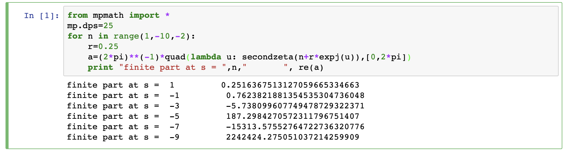
Refer to caption
Figure 8. Computation of the apparent value at s=1−2​ns=1-2n

where the implied precision is expected to hold, but is not guaranteed.

The first increasing and decreasing intervals of the function appear to be

d9↗−9↗c9↘b7↗−7↗b5↘d5↗−5↗c5↘b3↗−1↗1↘+∞d_{9}\nearrow-9\nearrow c_{9}\searrow b_{7}\nearrow-7\nearrow b_{5}\searrow d_{5}\nearrow-5\nearrow c_{5}\searrow b_{3}\nearrow-1\nearrow 1\searrow+\infty

After seen these plots Voros asked me to represent the function 2​Z​(s)​cos⁡π​s22Z(s)\cos\frac{\pi s}{2} that would be pole-free. We give here two pieces of this plot. This function vanishes at the points −2​n-2n and at points a2​n+1≈−(2​n+1)a_{2n+1}\approx-(2n+1)

and have a pole at s=1s=1

References

  • [1] C. F. Gauss, Demonstratio nova Theorematis omnem functionem algebraicam rationalem integram unius variabilis in factores reales primi vel secundi gradus resolvi posse, in Carl Friedrich Gauss Werke, Band III, p. 3–31, Göttingen, 1866.
  • [2] H. Mellin, Über die Nullstellen der Zetafunktion, Acta Soc. Fennicae (A) 10 n. 11 (1917). English translation in App. D in [14].
  • [3] H. Cramér, Studien über die Nullstellen der Riemannschen Zetafunktion, Mathematische Z. 4 (1919) 104–130.
  • [4] A. P. Guinand, A summation formula in the theory of prime numbers, Proc. London Math. Soc. (2) 50 (1948) 107–119.
  • [5] J. Delsarte, Formules de Poisson avec reste, J. Analyse Math. 17 (1966) 419–431.
  • [6] I. C. Chakravarty, The secondary zeta-functions, J. Math. Anal. Appl. 30 (1970) 280–294.
  • [7] I. C. Chakravarty, A proof of the prime number summation formula without assuming the Riemann hypothesis, Aequationes Math. 4 (1970) 384–394.
  • [8] I. C. Chakravarty, Certain properties of a pair of secondary zeta-functions, J. Math. Anal. Appl. 35 (1971) 484–495.
  • [9] I. C. Chakravarty, On the functional equation of the secondary zeta-functions, Aequationes Math. 14 (1976) 49–57.
  • [10] W. Gabcke, Neue Herleitung und explicite Restabschätzung der Riemann-Siegel-Formel, Mathematisch-Naturwissenschaftlichen Fakultät der Georg-August-Universität zu Göttingen, Dissertation, Göttingen 1979.
  • [11] A. Ivić, On certain sums over ordinates of zeta zeros, Bull. Cl. Sci. Math. Nat. Sci. Math. 26 (2001) 39–52.
  • [12] F. W. J. Olver, Introduction to Asymptotics and Special functions, Academic Press, New York, 1974.
  • [13] A. Voros, Zeta functions for the Riemann zeros, Ann. Institute Fourier,53 (2003) 665–699.
  • [14] A. Voros, Zeta functions over Zeros of Zeta Functions, Lecture Notes of the Unione Matematica Italiana, Springer, 2010.
  • [15] Y. L. Luke, The Special Functions and Their Approximations, Vol 1, Academic Press, 1959.
  • [16] E. T. Whittaker, G. N. Watson, A Course in Modern Analysis, Cambridge University Press, 1965.
  • [17] F. Johansson et al., mpmath: a Python library for arbitrary-precision floating-point arithmetic (version 1.1.0), December 2018. http://mpmath.org/. (documentation of secondzeta in mpmath).