Picket: Guarding Against Corrupted Data in Tabular Data during Learning and Inference
Abstract.
Data corruption is an impediment to modern machine learning deployments. Corrupted data can severely bias the learned model and can also lead to invalid inferences. We present, Picket, a simple framework to safeguard against data corruptions during both training and deployment of machine learning models over tabular data. For the training stage, Picket identifies and removes corrupted data points from the training data to avoid obtaining a biased model. For the deployment stage, Picket flags, in an online manner, corrupted query points to a trained machine learning model that due to noise will result in incorrect predictions. To detect corrupted data, Picket uses a self-supervised deep learning model for mixed-type tabular data, which we call PicketNet. To minimize the burden of deployment, learning a PicketNet model does not require any human-labeled data. Picket is designed as a plugin that can increase the robustness of any machine learning pipeline. We evaluate Picket on a diverse array of real-world data considering different corruption models that include systematic and adversarial noise during both training and testing. We show that Picket consistently safeguards against corrupted data during both training and deployment of various models ranging from SVMs to neural networks, beating a diverse array of competing methods that span from data quality validation models to robust outlier-detection models.
1. Introduction
Data quality assessment is critical in all phases of the machine learning (ML) life cycle. Both in the training and deployment (inference) stages of ML models, erroneous data can have devastating effects. In the training stage, errors in the data can lead to biased ML models (Koh et al. 2018; Schelter et al. 2019; Breck et al. [n.d.]; Baylor et al. 2017), i.e., models that learn wrong decision boundaries. In the deployment stage, errors in the inference queries can result in wrong predictions, which in turn can be harmful for critical decision making systems (Breck et al. [n.d.]; Steinhardt et al. 2017). ML pipelines need reliable data quality assessment during both training and inference to be robust to data errors.
We focus on tabular data and seek to develop a simple, plug-and-play approach to guard against corrupted data (including adversarially corrupted data) during both training and inference in ML pipelines. During training, our goal is to identify and filter corrupted examples from the data used to train a model, while during deployment, our goal is to flag erroneous query points to a pre-trained ML model, i.e., points that due to noise will result in incorrect predictions of the ML model. This work introduces a unified solution to guard against corrupted data for both the training and deployment stages of ML models.
Guarding against corrupted data in ML pipelines exhibits many challenges. First, detecting corrupted examples in the training data can be a hard exercise that requires developing methods that go beyond standard outlier detection mechanisms (Xue et al. 2010). Data poisoning techniques (Steinhardt et al. 2017; Koh et al. 2018; Muñoz-González et al. 2017; Biggio et al. 2012) attack models by adding a small fraction of adversarially crafted poisoned data to the training set. Any reliable mechanism that filters corruptions from a training data set should not only remove easy to detect outliers but also hard to detect poisoned data.
Second, online-detection of inference queries that yield a model misprediction due to corruption requires not only knowledge of the data quality, but also knowledge of the tolerance of the trained ML model to corruptions. The reason is that not all corruptions will flip the prediction of a trained ML model and different models exhibit different degrees of robustness to corruption. Moreover, adversarial noise may target specific subsets of the data or classes in the ML pipeline (Koh et al. 2018). For this reason, online-filtering of corrupted inference queries requires a method that takes both the downstream model and data quality into account.
The above challenges require rethinking the current solutions for identifying errors in data. The majority of outlier detection methods in the statistical literature (Xue et al. 2010; Liu et al. 2008; Chen et al. 2001) and error detection methods in the database literature (Heidari et al. 2019; Mahdavi et al. 2019) are not effective against adversarial corruptions (Koh et al. 2018). More advanced methods are required to defend against adversarial corruptions (Steinhardt et al. 2017). However, current methods are typically limited to real-valued data (Diakonikolas et al. 2017) and focus either on training (Diakonikolas et al. 2018) or inference (Roth et al. 2019; Grosse et al. 2017) but not both. Finally, recent techniques for data validation in ML pipelines that are deployed in industrial settings (Schelter et al. 2019; Breck et al. [n.d.]) rely on user-specified rule- or schema-based quality assertions evaluated over batches of data and it is unclear if they can support on-the-fly, single point validation, which is required during inference.
We present Picket , a framework for safeguarding against corrupted data during both the training and deployment stages of ML pipelines. Picket can be used in an offline manner to validate data that will be used for training but can also be used in an online manner to safeguard against corruptions for on-the-fly queries at inference time. We empirically demonstrate that Picket outperforms both state-of-the-art outlier detection mechanisms such as Robust Variational Autoencoders (Eduardo et al. 2020), and state-of-the-art methods for detection of adversarial corruption attacks during inference (Roth et al. 2019; Grosse et al. 2017). Our work makes the following technical contributions:
Self-Attention for Tabular Data Picket is built around PicketNet, a new deep learning-based encoder for mixed-type tabular data. PicketNet can model mixtures over numerical, categorical, and even text-based entries of limited length (e.g., descriptions). The goal of PicketNet is to learn the characteristics of the distribution governing the non-corrupted data on which the ML pipeline operates and it is used in Picket to distinguish between clean data points and corrupted ones. The architecture of PicketNet builds upon the general family of Transformer networks (Vaswani et al. 2017) and introduces a new multi-head self-attention module (Vaswani et al. 2017) over tabular data. This module follows a stream-based architecture that is able to capture not only the dependencies between attributes at the schema-level but also the statistical relations between cell values—it follows a schema stream and value stream architecture. We find that compared to schema-only models, PicketNet’s two-stream architecture is critical for obtaining accurate predictions across diverse data sets.
Robust Training over Arbitrary Corruptions We show how to learn a PicketNet model without imposing any extra labeling burden to the user and by operating directly on potentially corrupted data (i.e., we do not not require access to clean data to learn the non-corrupted data distribution). We achieve that by using a robust self-supervised training approach that is robust to corrupted data points (including adversarial points). As with standard self-supervision, the context captured in the data is used as the supervision signal. The training procedure for PicketNet monitors the reconstruction loss of tuples in the input data over early training iterations and uses related statistics to identify suspicious data points. These points are then excluded from subsequent iterations during training.
A Plugin to ML Pipelines We demonstrate how Picket can serve as a “plugin” that safeguards against corrupted data in different ML pipelines during both training and inference. We evaluate Picket over multiple data sets with different distributional characteristics and consider different types and magnitudes of corruption, ranging from simple random noise to adversarial attacks that explicitly aim to harm the performance of downstream ML models. We find that Picket provides a reliable mechanism for detecting data corruptions in ML pipelines: Picket consistently achieves an area under the receiver operating characteristic curve (AUROC) score of above or close to 80 points for detecting corrupted data across different types of noise and ML models.
2. Background
Data Corruption Models We consider data corruption due to random, systematic, and adversarial noise.
1. Random noise is drawn from some unknown distribution that does not depend on the data. Random noise is not predictable and cannot be replicated in a repeatable manner. While, many ML models are robust to purely random noise during training, high-magnitude random noise can still lead to false predictions, and hence is of interest to our study.
2. Systematic noise depends on values in the data and leads to repeated errors in data samples. This type of noise biases the distribution of the data. Systematic noise can skew the distribution of the data, and this bias can potentially harm the performance of an ML model depending on the importance of the corrupted features to the downstream prediction task.
3. Adversarial noise contaminates the data to explicitly mislead ML models and harm their performance. At training time, adversarial noise corrupts the training points to force a model to learn a bad decision boundary; at test time, adversarial noise corrupts the input queries in a manner that will lead to a false prediction by the model. It usually depends on the data and the target model, although some types of adversarial noise may work well across different models.
Dealing with Corrupted Data in ML The most common approach to deal with corrupted data during training is to identify corrupted samples and remove them from the training set. This process is referred to as filtering. Given a training data set , filtering identifies a set of clean data points to be used for training. Common filtering mechanisms rely on outlier detection methods (Liu et al. 2008; Chen et al. 2001; Eduardo et al. 2020). In addition, recent filtering methods focus on adversarial corruptions over real-valued data (Eduardo et al. 2020; Diakonikolas et al. 2017). Finally, there are data validation modules for ML platforms (Baylor et al. 2017; Schelter et al. 2019; Breck et al. [n.d.]) that rely on user-defined rules and simple statistics to check the quality of data batches. The statistical tests used by these methods are subsumed by outlier detection methods and user-defined quality rules are out of the scope of this work. For inference, apart from outlier detection methods, there are methods that accept or reject inference queries by using statistical tests that compare the query to clean data (Grosse et al. 2017) or by considering variations in a model’s internal data representation (Roth et al. 2019). We also consider the online detection of inference queries that result in wrong predictions due to corruption.
Self-Supervision In self-supervised learning systems (Devlin et al. 2018; Su et al. 2020), the learning objective is to predict part of the input from the rest of it. A typical approach to self-supervision is to mask a portion of the input, and then let the model reconstruct the masked portion based on the unmasked parts. By self-supervision, a model learns to capture dependencies between different parts of the data. Self-supervised learning is a subset of unsupervised learning in a broad sense since it does not need human supervision.
Multi-Head Self-Attention Models with multi-head self-attention mechanism learn representations for structured inputs e.g., a tuple or a text sequence, by capturing the dependencies between different parts of the inputs (Vaswani et al. 2017). One part can pay different levels of attention to other parts of the same structured input. For example, consider the text sequence “the dog wears a white hat”, the token “wears” pays more attention to “hat” than “white” although “white” is closer in the sequence. The attention mechanism can also be applied to tuples that consist of different attributes (Wu et al. 2020). Multi-head self-attention takes an ensemble of different attention functions, with each head learning one.
We provide a brief review of the multi-head self-attention model (Vaswani et al. 2017). Let be the embedding of a structured input with tokens. Each token is transformed into a query-key-value triplet (, , ) by three learnable matrices , and . The query , key , and value are real-valued vectors with the same dimension . The output of a single head for the token is , a weighted sum of all the values in the sequence, where . The attention pays to is determined by the inner product between and . Multiple heads share the same mechanism but have different transformation matrices. The outputs of all the heads are concatenated and transformed into the final output by an output matrix , which is also learnable.
3. Overview of Picket
We review Picket’s functionalities during the training and inference phases of a ML pipeline. An overview diagram of Picket’s core components and functionalities is shown in Figure 1. The corresponding pseudo-code is shown in Algorithm 1.

Input: dataset , downstream model type and configuration ;
Inference Time (Offline Phase):
Input: filtered dataset , trained downstream model ;
Inference Time (Online Phase):
Input: data stream , trained downstream model , trained PicketNet , victim sample detectors ;
Guarding against Corrupted Data in Training
We consider a tabular data set with training examples. Let be a sample (tuple) in with attributes. These attributes correspond to the features that are used by the downstream model. For each we denote its clean version; if is not corrupted then .
We assume that contains clean and corrupted samples and that the fraction of corrupted samples is always less than half. The goal of Picket is to filter out the corrupted samples in and construct a clean set of examples to be used for training a downstream model. Without loss of generality we assume that Picket performs filtering over once. This process can be repeated for data batches over time. We next describe how we construct in Picket.
Picket follows the next steps: First, Picket learns a self-supervised PicketNet model that captures how data features are distributed for the clean samples. Picket does not require human-labelled examples of corrupted or clean data. During training, Picket records the reconstruction loss across training epochs for all points in . After training of , we analyze the reconstruction loss progression over the first few training epochs to identify points in that are corrupted (see Section 5 for details). Set is constructed by removing these corrupted points from . We also proceed with training on . The pre-trained PicketNet model is used to detect corruptions during inference.


Guarding against Corrupted Data in Inference
We consider a trained model that serves inference queries over data points with the same attributes as in the training phase of the ML pipeline.
We define a victim sample to be a point such that but , i.e., the input sample is corrupted and it gets misclassified due to corruption. We show an example that illustrates the difference between non-victim and victim samples according to our definition in Figure 2.
The goal of Picket is to solve the following problem: Given an already-trained classifier , for each sample that comes on the fly, we want to tell if it is a good sample or it is a victim sample and will be misclassified due to corruption, i.e., we want to detect if . We assume access to data set and model output by Picket for safeguarding during the training phase of the ML pipeline in hand. We then adopt a two-phase approach, offline and online phase, to solve the aforementioned problem.
We now focus on the offline phase. Given the trained model , data set , and model , we learn a victim-sample detector for each class in the prediction task in-hand. Each victim-sample detector is a binary classifier that detects if an input sample will be misclassified by due to corruption. The victim-sample detectors operate on an extended feature set: Beyond the original features of the inference query we add additional features corresponding to the reconstruction-loss obtained by masking each feature in turn and applying model to predict it back.
During the online phase, we use model and the victim-sample detectors over a stream of incoming inference queries to identify victim samples. Picket performs the following: for each incoming point , Picket evaluates classifier on to obtain an initial prediction . Picket also uses to compute the reconstruction-loss vector for the features of . The extended feature vector containing the original features of and the reconstruction loss features are given as input to the victim sample detector for the class that corresponds to the prediction . Using this input, the detector identifies if point corresponds to a victim sample. If the point is not marked as suspicious the final prediction is revealed downstream, otherwise the inference query is flagged.
4. The PicketNet Model
Picket uses a new two-stream multi-head self-attention model to learn the distribution of tabular data. We refer to this model as PicketNet. The term stream refers to a path in a neural network that focuses on a specific view of the input data. For example, standard attention mechanism is one stream that learns value-based dependencies between the parts of the input data (see Section 2). Combining multiple streams, where each stream focuses on learning a different view of the data, has been shown to achieve state-of-the-art results in natural language processing tasks (Yang et al. 2019) and computer vision tasks (Simonyan and Zisserman 2014) but has not been applied on tabular data. PicketNet introduces a new two-stream model for tabular data and proposes a robust, self-supervised training procedure for learning this model.
4.1. Model Architecture
PicketNet contains two streams: a schema stream and a value stream. The schema stream captures schema-level dependencies between attributes of the data, while the value stream captures dependencies between specific data values. A design overview of PicketNet is shown in Figure 3 with details of the two streams. The input to the network is a mixed-type data tuple with attributes .
The first level of Picket obtains a numerical representation of tuple . To capture the schema- and value-level information for , we consider two numerical representations for each attribute : 1) a real-valued vector that encodes the information in value , denoted by , and 2) a real-valued vector that encodes schema-level information of attribute , denoted by . For example, a tuple with two attributes is represented as . To convert to , PicketNet uses the following process: The encoding for each attribute value is computed independently. We consider 1) categorical, 2) numerical, and 3) textual (short-text) attributes. For categorical attributes, we use a learnable lookup table to get the embedding for each value in the domain. This lookup table is learned jointly with all other components of PicketNet. For numerical attributes, we keep the raw value as one dimension and pad the other dimensions with zeros. For text attributes, we train a fastText (Bojanowski et al. 2017) model over the corpus of all the texts and apply SIF (Arora et al. 2019) to aggregate the embedding of all the words in a cell. The initial embedding vectors are inputs to the value-level stream.
Each vector serves as a positional encoding of the attribute associated with index . Positional encodings are used to capture high-level dependencies between attributes. is consistent for attribute in all examples, i.e., it does not change as the values in different examples vary. Hence, it captures common dependencies at the schema level. Each corresponds to a trainable vector that is initialized randomly and is fed as input to the schema stream.
We now describe subsequent layers of our model. These layers consider the two attention streams and form a stack of self-attention layers. The output of the previous layer serves as the input to the next layer. Self-attention layer takes the value vector and positional encoding to learn a further representation for attribute and its value . After each attention layer, the outputs of the two streams are aggregated and fed as input to the value-level stream of the next layer, while the schema stream still takes as input the positional encoding. The output of the value stream and that of the schema stream are computed as:
where MHS represents the multi-head attention function followed by a feed-forward network and , , are linear transformations that transform the input into query, key, or value vectors by the corresponding weight matrices for , , and . Finally, are matrices formed by packing the query, key and value vectors from their inputs.
The difference between the two streams is that the query in the schema stream corresponds to the positional encoding, therefore it learns higher-level dependencies. For the value stream the input to the next level is the sum of the outputs from the two streams: ; for the schema stream the input to the next level corresponds to a new positional encoding that does not depend on the previous layers. If layer is the last layer, is the final representation for attribute value .

4.2. Training Process
We learn PicketNet using the noisy data set without any human-labeled examples of corrupted or clean data. Training follows a self-supervised learning objective.
Self-Supervised Training For each point in , we mask one of the attributes and then try to reconstruct it based on the values of the other attributes in the same tuple. Other attributes may still contain noisy data or missing values. The attributes are masked in turn following an arbitrary order. The training is also multi-task since the reconstruction of each attribute forms one learning task.
We use different types of losses for the three types of attributes to quantify the quality of reconstruction. Consider a sample whose original value of attribute is . If is numerical, its a one-dimensional value, and hence, the reconstruction of the input value is a regression task: We apply a simple neural network on the output to get an one-dimensional reconstruction , and use the mean squared error (MSE) loss: .
For categorical or text-based attributes we use the cross-entropy loss. Consider a tuple and its attribute . For its attribute value let be the base-embedding before passing through the attention layers of PicketNet, and the contextual encoding of value after pushing tuple (with attribute masked) through PicketNet. Given tuple , we randomly select a set of other values from the domain of attribute . We consider the training loss associated with identifying as the correct completion value from the set of possible values . To compute the training loss we use the cosine similarity between and the input encoding for each , then we apply the softmax function over the similarities and calculate the cross-entropy (CE) loss:
where is the cosine similarity between and .
Loss-based Filtering to Ensure Robust Training
The data used to learn PicketNet can be corrupted, in which case self-supervised learning might lead to a biased model due to the presence of noise.
To make learning robust to noisy input, we use a loss-based filtering mechanism to detect and ignore corrupted data during training of a PicketNet model. The process we use follows the next steps:
1. Warm-start PicketNet by training over for epochs.
2. Train PicketNet over for epochs and, for each sample in , record the epoch-wise average loss for each attribute , .
3. For each sample, aggregate the losses attribute-wise by where computes the median over all points in .
4. Put a sample into set if its aggregated loss is less than or greater than , where and are pre-specified thresholds; is the set of samples to be removed.
5. Train PicketNet over until convergence.
The thresholds and control the sensitivity of the detection. In practice, we can set and based on a relatively clean validation set. A common strategy is setting their values based on the validation set so that the false positive rate (FPR) is under some value (e.g. 5%). When a relatively clean validation set is not available, the thresholds can be set based on the histogram of the reconstruction loss. Filtering out abnormal peaks and low density tails in the histogram is a natural strategy, and we validate the effectiveness of it in Section 6.4.
When we do the attribute-wise aggregation, we normalize the loss of each attribute by dividing with the median of it to bring different types of losses to the same scale. The normalized loss characterizes how large the loss is relative to the average level loss in that attribute. We use the median since it is robust against extremely high or low values, while the mean can be significantly shifted by them.

The filtering is two-sided because randomly or systematically corrupted samples and adversarially crafted (poisoned) samples have different behaviors during the early training stage. Outliers with random or systematic noise are internally inconsistent and thus have high reconstruction loss in the early training stage of PicketNet. However, poisoned samples tend to have unusually low reconstruction loss. The reason is that poisoned data tend to be concentrated on a few locations to be effective and appear normal, as is pointed out by Koh et al. (Koh et al. 2018). Such concentration forces deep networks such as PicketNet to fit quickly and therefore the reconstruction loss in the early stage is lower than that of the clean samples. We confirm this hypothesis experimentally. Figure 4 shows the distribution of the reconstruction loss for 1) clean, 2) randomly and systematically corrupted, and 3)poisoned samples for a real-world dataset. The noise used in this illustrative example follows the procedure described in Section 6.1. The three distributions have notable statistical distances. Hence, we need to remove samples with high loss to capture random or systematic corruptions, and samples with abnormally low loss to defend against poisoning attacks.
5. Detecting Data Corruptions
The reconstruction loss of PicketNet is the key to training time and inference time detection. We now provide more details on these functions of Picket.
Detecting Corrupted Training Data Detection of corrupted training data follows directly from the training procedure of PicketNet described in the previous section (Section 4.2). Given an ML pipeline that aims to learn a model for a downstream task, we 1) first train a PicketNet model over the data considered for training and 2) only use the data points that are not filtered during the training of PicketNet to train the downstream model . This approach allows us to apply Picket to any training pipeline regardless of the downstream model. Effectively, the pre-trained PicketNet is used as an encoder capable to detect outlier points. As we show in Section 6, our approach is effective across different types of ML models. For adversarially poisoned training data, we find that using Picket as a filter before training, allows us to train downstream ML models that exhibit similar performance to that of models trained on non-corrupted data.
Victim Sample Detection for Inference We now describe how we construct the victim sample detectors to safeguard against corruptions during inference for a trained classifier (see Section 3). For each class in the downstream classification task, we build a detector to identify victim samples, i.e., samples that will misclassify due to corruption of the feature values. The detectors are binary classifiers. In our experiments, we use logistic regression models with regularization parameter as detectors.
At inference time, the victim sample detectors are deployed along with the downstream model and a pre-trained PicketNet model . Whenever a sample comes, the downstream model gives the prediction . The corresponding detector takes into account and the feature-wise reconstruction loss (not aggregated) from and decides if should be marked as suspicious.
We learn the victim-sample detectors by using a data set with artificially corrupted data points. We describe this process below; notice that no human-labeled data is required. We start from the filtered data output by Picket during the training phase of the ML pipeline. We first apply the already-trained classifier on all points in and obtain a subset of points for which returns the correct prediction, i.e., . We denote this subset . Moreover, we partition into sets , one for each class of the downstream prediction class. For each partition, we use the points in to construct artificial victim samples and artificial noisy points for which returns the correct prediction despite the injection of noise. We discuss the artificial noise we inject in detail in Section 6.1. Let and be the set of artificial victim samples and the set of noisy but correctly classified sample generated from respectively. To construct these two data sets we select a random point from and inject artificial noise to obtain a noisy version ; we then evaluate and if we assign the generated point to otherwise we assign it to . We iteratively perform the above process for randomly selected points in until we populate sets and with enough points such that . Given these three sets, we construct a new augmented data set . We extend the feature vector for each point in by concatenating it with the reconstruction loss vector obtained after passing each point through the trained PicketNet . We also assign to it a positive label (indicative that we will obtain a correct prediction) if it originated from or and a negative label (indicating that we will obtain a wrong prediction) if it originated from . The output of this procedure is the training data for the victim sample detector . We repeat the above process for each class .
Ideally, the artificial noise that we inject should have the same distribution as that in the real-world case. However, it is impossible to know the exact noise distribution in advance. A practical solution is injecting mixed-type artificial noise to help the detectors learn an approximate boundary between good and victim samples. As mentioned we discuss the artificial noise we consider in Section 6.1. We validate the effectiveness of mixed-type artificial noise in Section 6.4.
6. Experiments
We evaluate how effective Picket and a diverse array of competing methods are on detecting different types of corruption in ML pipelines during the training and inference phases. We also provide several micro-benchmarks over different design choices in Picket. Finally, we report the runtime and discuss the scalability.
6.1. Experimental Setup
Datasets We consider six datasets with different mixtures of numerical, categorical, and text-based attributes. These datasets are obtained from the UCI repository (Dua and Graff 2017) and the CleanML benchmark (Li et al. 2019). All datasets focus on binary classification tasks. The characteristics of these datasets are summarized in Table 1. A detailed description of the datasets is as follows.
- •
Wine: The dataset consists of statistics about different types of wine based on physicochemical tests. The task is to predict if the quality of a type of wine is beyond average or not. The features are purely numerical.
- •
Adult: The dataset contains a set of US Census records of adults. The task is to predict if a person makes over $50,000 per year. The features are a mixture of categorical and numerical attributes.
- •
Marketing: The dataset comes from a survey on household income consisting of several demographic features. The task is to predict whether the annual gross income of a household is less than $25,000. The features are purely categorical.
- •
Restaurant: The dataset contains information of restaurants from Yelp. The task is to predict if the price range of a restaurant is “one dollar sign” on Yelp. The features are a mixture of categorical values and textual description,
- •
Titanic: The dataset contains personal and ticket information of passengers. The task is to predict if a passenger survives or not. The features are a mixture of numerical, categorical and textual attributes.
- •
HTRU2: The dataset contains statistics about a set of pulsar candidates collected in a universe survey. The task is to predict if a candidate is a real pulsar or not. The features are purely numeric.
The last dataset, i.e., HTRU2, is purely numerical and we use it in the context of adversarial noise. The datasets above are the ones we use for most of our experiments. In addition, we use Food labeled by (Heidari et al. 2019) for real noise, and Alarm (Herskovits 1992) for the study of scalibility. We consider downstream ML pipelines over these datasets that use 80% of each dataset as the training set, and the rest as test data. To reduce the effect of class imbalance, we undersample the unbalanced datasets where over 70% of the samples belong to one class. The numerical attributes are normalized to zero mean and unit variance before noise injection.
| Dataset | Size | Numerical Attributes | Categorical Attributes | Textual Attributes |
|---|---|---|---|---|
| Wine | 4898 | 11 | 0 | 0 |
| Adult | 32561 | 5 | 9 | 0 |
| Marketing | 8993 | 0 | 13 | 0 |
| Restaurant | 12007 | 0 | 3 | 7 |
| Titanic | 891 | 2 | 5 | 3 |
| HTRU2 | 17898 | 8 | 0 | 0 |
Noise Models In our experiments, we consider different types of noise: 1) random, 2) systematic, 3) adversarial noise, and 4) common errors in real-world datasets.
Random and systematic noise are model agnostic and only take into account the dataset. For random and systematic noise, we corrupt fraction of the cells in the noisy samples. We now provide a detailed description of the random and systematic noise generation process we consider.
Random Noise: For a categorical or textual attribute, the value of a corrupted cell is flipped to another value in the domain of that attribute. For a numerical attribute, we add Gaussian noise to the value of a corrupted cell, with zero mean and standard deviation of , where is a constant.
Systematic Noise: For categorical and textual data, we randomly generate a predefined function which maps the value of the cell to be corrupted to another value in the same domain. The mapping function depends on both the original value in that attribute and that in another pre-specified attribute, i.e., where . For a numerical attribute, we add a fixed amount of noise to the value of a corrupted cell, where is a constant.
We consider three settings with respect to the fraction of corrupted cells in the noisy samples (and the magnitude of error in the case of numerical values) for random and systematic noise, which we refer to as High (, ), Medium (, ) and Low (, ).
For adversarial attacks, we use methods that take into account specific ML models. Specifically, we use data poisoning techniques at training, and evasion attack methods at inference. For the part of our evaluation that focuses on training time, we generate poisoned samples using the back-gradient method (Muñoz-González et al. 2017). Since, this type of poisoning is specific to different downstream models we consider different dataset-model combinations in our evaluation. For the part of our evaluation that focuses on inference time, we use the projected gradient descent (PGD) attack (Madry et al. 2018a), a popular and effective white-box evasion attack method, to generate adversarial test samples. We use the implementation of PGD attack from (Nicolae et al. 2018). The corruption injected by the PGD attack is bounded by an infinity norm of . The step size is and the number of iterations is .
For common errors in real-world datasets, we consider missing values that cannot be detected during pre-processing (e.g. 99999 instead of NaN), multiplicative scaling of attributes (e.g. due to accidental changes of units), and typos in textual or categorical attributes. We synthesize this kind of noise as follows:
- (1)
If the corrupted cell is numerical, with probability 1/3 it will be 10 times larger, and with the same probability it will be 10 times smaller. Otherwise, the cell will contain a missing value.
- (2)
If the corrupted cell is categorical or textual, with probability 1/2 one of the character will be replaced by a random character. Otherwise, the cell will contain a missing value.
For this kind of noise, we set the fraction of corrupted cells in the noisy samples as . We also include Food, a dataset that contains real-world errors with manually labeled ground truth (Heidari et al. 2019). It has 3 numerical, 6 categorical and 5 textual attributes. Out of its 3000 samples, 30.3% are corrupted.
As discussed in Section 5, we use artificially generated noise to create the training data for learning the victim-sample detectors. We now describe the type of noise we consider. Recall that we consider access to the set of clean sample and we augment this set with artificially corrupted data. We emphasize that the noise is always different than the noise considered in the training data. Since we assume that the type of noise in the test set is unknown in advance, the artificial noise contains a mixture of different levels of random noise (, , ). We additionally augment with samples corrupted by random noise () and adversarial samples generated by Fast Gradient Sign Method (FGSM) (Goodfellow et al. 2015)(noise bounded by an infinite norm of ) to defend against adversarial noise. This corruption is different from the PGD attack considered during inference to ensure that we evaluate against a different noise distribution during online inference.
Downstream ML Models We consider the following downstream models: 1) A Logistic regression (LR) model with regularization parameter 1.0; 2) A Support Vector Machine (SVM) with a linear kernel and regularization parameter 1.0; 3) A fully-connected neural network (NN) with 2 hidden layers of size 100. We use a small model with 1 hidden layer of size 10 when we perform poisoning attacks due to the runtime complexity of the attack algorithm. The downstream models we choose cover different optimization objectives (logistic/hinge loss and convex/non-convex optimization objectives) and exhibit different robustness. Numerical attributes are encoded as their raw values for downstream models. Categorical and textual attributes are encoded in the same way as in Picket.
Training-Time Baselines We compare against three unsupervised outlier detection methods as follows: 1) Isolation Forest (IF) (Liu et al. 2008), an approach similar to Random Forests but targeting outlier detection, 2) One-Class SVM (OCSVM) (Chen et al. 2001) with a radial basis function kernel, and 3) Robust Variational Autoencoders (RVAE) (Eduardo et al. 2020), a state-of-the-art generative model used for outlier detection on mixed-type tabular data. For IF, we use 100 base estimators in the ensemble. For RVAE, we use the default hyperparameter recommended by Eduardo et al. (Eduardo et al. 2020), which has 972,537 parameters. Note that the capacity of the RVAE model used in our experiments is larger than PicketNet, which has 382,722 parameters. The detailed hyper-parameters we use for PicketNet is reported in Appendix A.1.
Inference-Time Baselines We compare against: 1) victim-sample detectors based, 2) naïve confidence-based, and 3) adversarial data detection methods.
Methods based on per-class victim sample detectors follow the same strategy as Picket but use different features. We consider: 1) Raw Feature (RF), the binary classifiers only use the raw features of the data; 2) RVAE, the binary classifiers use only the cell-level probability of being outliers provided by RVAE as features; 3) RVAE+, the classifiers use a combination of the features from the two methods above.
We also consider the next naïve methods: 1) Calibrated Confidence Score (CCS), which assumes that the predictions of the downstream model have lower confidence for victim samples than clean samples. We calibrate the confidence scores of the downstream models using temperature scaling (Guo et al. 2017). 2) -Nearest Neighbors (KNN), which assumes that a victim sample has a different prediction from its neighbors. We use different distances for different types of attributes. For numerical attributes, the distance is if , where is the difference between two normalized values; the distance is if . For categorical attributes, we use the Hamming distance and for text attributes the cosine distance. We set to .
We consider two methods of adversarial sample detection: The Odds are Odd (TOAO) (Roth et al. 2019), which detects adversarial samples based on the change in the distribution of the prediction logit values after the injection of random noise. It adds Gaussian, Bernoulli, and Uniform noise of different magnitude and takes the majority vote of all noise sources. 2) Model with Outlier Class (MWOC) (Grosse et al. 2017), which assumes that the feature distribution of adversarial samples is different from that of benign samples and adds a new outlier class to the downstream model to characterize the distribution of adversarial samples.
For a fair evaluation of baselines against Picket, we also reveal the augmented version of used to learn the victim-sample detectors in Picket to competing methods so that they fine-tune their models to noise (RF, RVAE, RVAE+, MWOC, Picket), or use it to find a good threshold (CCS, KNN, TOAO).
Metrics For training-time outlier detection, we report the area under the receiver operating characteristic curve (AUROC). We use AUROC since it is an aggregate measure of performance across all possible threshold settings. We also consider the test accuracy of downstream models. For victim sample detection, we report the scores of the classification between correctly classified samples and victim samples.
Evaluation Protocol All experiments are repeated five times with different random seeds that control train-test split and noise injection; the mean is reported. We also perform one-sided paired t-tests when we compare the examined methods. A method is considered significantly better than another one if the p value is less than 0.05. In addition, we provide a cross-validation-based evaluation in Appendix A.3 that examine the performance of outlier detection on unseen data.

6.2. Training-Time Evaluation
We evaluate the performance of different methods on detecting erroneous points in the training data. We then evaluate how these methods affect the performance of downstream models. We also provide a study on synthetic datasets in Appendix A.2 to see how these outlier detection methods perform when certain aspects of the data and noise vary.

Detecting Corrupted Training Examples Figures 5, 6, and 7 show the AUROC obtained by the methods for different types of noise, when 20% of the samples are corrupted. The results for random and systematic noise correspond to Medium level noise. Results for Low and High levels are reported in Appendix A.5. For Figure 7, note that the poisoned samples are model-specific and hence we report the dataset model combination on the x-axis. Due to data poisoning being limited to numerical data, we only evaluate on Wine and HTRU.

As shown, Picket is the only approach that consistently achieves an AUROC of close to or more than 0.8 for all datasets and for all noise settings. Other methods achieve comparable performance in some settings but they are not consistent across diverse settings. IF and OCSVM perform poorly on datasets with textual attributes (Restaurant and Titanic) due to their limited capacity to handle text-based attributes. RVAE works quite well under random noise, but its performance drops a lot when it comes to systematic noise, which shows that it is not robust against noise that introduces bias. In the presence of poisoned data, we find that IF performs well on Wine but poorly on HTRU2, but OCSVM shows the opposite. A possible reason is that the two datasets exhibit different types of correlation between attributes, and the two methods are good at capturing only one of them. RVAE shows poor performance for both datasets.
For common errors in the real world, the results are shown in Figure 8. We add synthetic errors of this type to Titanic and Restaurant, where 20% are corrupted. We choose these two because they contain textual attributes for typos. We also report the results on Food with real-world noise. We can see that on Restaurant and Titanic, Picket outperforms the others by more than 6 points. On Food, all the methods perform poorly. This is because the noise level in Food is very low, and therefore hard to detect. In fact, the real noise contained in Food does not have a significant effect on the downstream models (as is shown in Table 22).
We also study how the fraction of corrupted samples affects the performance of detection (see Appendix A.4). We find that Picket keeps a relatively consistent performance when the fraction of corrupted samples varies.

Effect on Downstream Models We also study the effect of different filtering methods on the downstream models. For each method, we filter 20% of the samples with highest outlier scores, and train different downstream models on the resulting training set. For each dataset, the test set is fixed and contains only clean data. As reference points, we also include the test accuracy when 1) the training data is clean without corruption (CL), and 2) the training data is corrupted but no filtering (NF) is performed. Note that in the CL and NF cases, the sample size is different from the rest since there is no filtering in these two. As a side effect of filtering, the decrease in sample size will also affect the performance of the downstream model. We want to include such an effect in our comparison, so we use CL and NF with no sample filtered out as baselines.
| Dataset | DM* | IF | OCSVM | RVAE | Picket | CL | NF |
|---|---|---|---|---|---|---|---|
| Wine | LR | 0.7261 | 0.6976 | 0.7051 | 0.7312 | 0.7349 | 0.6745 |
| SVM | 0.7286 | 0.6933 | 0.7082 | 0.7310 | 0.7386 | 0.6727 | |
| NN | 0.7210 | 0.6894 | 0.7035 | 0.7320 | 0.7365 | 0.6722 | |
| HTRU2 | LR | 0.8884 | 0.9015 | 0.8811 | 0.9067 | 0.9396 | 0.8799 |
| SVM | 0.8884 | 0.8979 | 0.8887 | 0.9232 | 0.9424 | 0.8832 | |
| NN | 0.8671 | 0.8707 | 0.8643 | 0.9000 | 0.9280 | 0.8646 |
- •
*DM = Downstream Model.
First, we consider the case of data poisoning since this type of corruption has the most significant effect on the downstream models. We measure the test accuracy of the downstream models when poisoned data are injected into the training stage. The results are shown in Table 2. If we compare CL with NF we see an average drop of six accuracy points if corruptions are ignored and no filtering is applied. We find that all methods reduce the negative impact of the poisoned data and bring up the test accuracy. Nevertheless that Picket outperforms all competing baselines and yields test time accuracy improvements of more than three points in some cases. We see that Picket is able to recover most of the accuracy loss for all models in the Wine dataset and comes very close to CL for HRTU2. All other methods exhibit smaller accuracy improvements and do not exhibit consistent behavior across datasets.
We also consider the cases of random and systematic noise, as well as common errors in the real world. These types of noise do not directly attack the downstream model. Moreover, most ML models are somewhat robust to these types of noise. As a result, we expect to see a small gap in the test accuracy between CL and NF, and all methods to perform comparably. We report the results in these setups in Appendix A.6 for completeness.
6.3. Inference-Time Evaluation
We evaluate the different methods on victim sample detection under different types of noise. The scores under random (Medium level), systematic (Medium level), adversarial noise and common errors in the real world are reported in Table 3, 4, 5 and 6. Food with real-world noise is not reported since we cannot find enough victim samples from it. We report results for High and Low noise in Appendix A.7.
| Dataset | DM* | RF | RVAE | RVAE+ | CCS | KNN | TOAO | MWOC | Picket |
|---|---|---|---|---|---|---|---|---|---|
| Wine | LR | 0.7690 | 0.7786 | 0.8172 | 0.6667 | 0.6686 | 0.6813 | 0.7150 | 0.8094 |
| SVM | 0.7812 | 0.7859 | 0.8254 | 0.6667 | 0.6750 | 0.6858 | 0.7622 | 0.8223 | |
| NN | 0.7125 | 0.7470 | 0.7833 | 0.5896 | 0.6669 | 0.5107 | 0.6988 | 0.7631 | |
| Adult | LR | 0.8352 | 0.7403 | 0.8489 | 0.6692 | 0.7866 | 0.2224 | 0.6725 | 0.8602 |
| SVM | 0.8434 | 0.7416 | 0.8553 | 0.6688 | 0.8060 | 0.4696 | 0.6215 | 0.8658 | |
| NN | 0.8131 | 0.7127 | 0.8315 | 0.5117 | 0.6891 | 0.3216 | 0.7132 | 0.8411 | |
| Restaurant | LR | 0.7726 | –# | – | 0.7403 | 0.6456 | 0.6457 | 0.7459 | 0.8266 |
| SVM | 0.6854 | – | – | 0.6796 | 0.6628 | 0.6596 | 0.5580 | 0.7618 | |
| NN | 0.7605 | – | – | 0.6994 | 0.6609 | 0.6110 | 0.7025 | 0.8203 | |
| Marketing | LR | 0.8366 | 0.6623 | 0.8403 | 0.7567 | 0.7815 | 0.6666 | 0.7996 | 0.8549 |
| SVM | 0.8461 | 0.6689 | 0.8501 | 0.7527 | 0.7886 | 0.5133 | 0.8109 | 0.8607 | |
| NN | 0.7931 | 0.6650 | 0.8029 | 0.6588 | 0.7050 | 0.6648 | 0.7265 | 0.8162 | |
| Titanic | LR | 0.8257 | – | – | 0.6990 | 0.6562 | 0.1409 | 0.7736 | 0.8424 |
| SVM | 0.8482 | – | – | 0.6658 | 0.6436 | 0.4652 | 0.7932 | 0.8528 | |
| NN | 0.8393 | – | – | 0.6631 | 0.6387 | 0.2575 | 0.7566 | 0.8483 |
- •
*DM = Downstream Model. #RVAE is not applicable to text attributes.
From the tables, we can see that Picket has the best performance in most cases. By comparing RF and our method, we show that the reconstruction loss features provided by PicketNet are good signals to help identify victim samples. Such signals are better than those provided by RVAE since our method outperforms RVAE+ most of the time. TOAO performs consistently poorly since the assumption it relies on does not hold for the downstream models and datasets we consider. It works for image classification with complex convolutional neural networks under adversarial settings since adding random noise to images could eliminate the effect of adversarial noise. However, for tabular datasets and models which are not that complex, especially when the noise is not adversarial, adding random noise does not make a big difference. Another method from the adversarial learning literature (MWOC) works well in some cases even if the noise is not adversarial.
| Dataset | DM* | RF | RVAE | RVAE+ | CCS | KNN | TOAO | MWOC | Picket |
|---|---|---|---|---|---|---|---|---|---|
| Wine | LR | 0.6883 | 0.4987 | 0.6619 | 0.6667 | 0.6499 | 0.3152 | 0.7937 | 0.7046 |
| SVM | 0.6785 | 0.5056 | 0.6630 | 0.6667 | 0.6325 | 0.3399 | 0.7957 | 0.6973 | |
| NN | 0.6760 | 0.6134 | 0.5689 | 0.6865 | 0.6659 | 0.3765 | 0.7190 | 0.6034 | |
| Adult | LR | 0.8281 | 0.6960 | 0.8342 | 0.6695 | 0.7488 | 0.1864 | 0.7430 | 0.8501 |
| SVM | 0.8414 | 0.6729 | 0.8428 | 0.6694 | 0.7900 | 0.3617 | 0.6646 | 0.8643 | |
| NN | 0.8108 | 0.6534 | 0.8245 | 0.5439 | 0.6808 | 0.2195 | 0.7850 | 0.8336 | |
| Restaurant | LR | 0.7773 | –# | – | 0.7419 | 0.6524 | 0.6496 | 0.7487 | 0.8255 |
| SVM | 0.7275 | – | – | 0.7093 | 0.6475 | 0.6356 | 0.6125 | 0.7845 | |
| NN | 0.7628 | – | – | 0.7010 | 0.6579 | 0.6051 | 0.7003 | 0.8126 | |
| Marketing | LR | 0.8358 | 0.6504 | 0.8403 | 0.7623 | 0.7770 | 0.6090 | 0.8068 | 0.8514 |
| SVM | 0.8501 | 0.6575 | 0.8552 | 0.7716 | 0.7817 | 0.6185 | 0.8208 | 0.8638 | |
| NN | 0.8036 | 0.6355 | 0.8098 | 0.6649 | 0.7074 | 0.6635 | 0.7035 | 0.8118 | |
| Titanic | LR | 0.8376 | – | – | 0.7349 | 0.6493 | 0.4076 | 0.7901 | 0.8438 |
| SVM | 0.8224 | – | – | 0.6674 | 0.6387 | 0.5592 | 0.7593 | 0.8412 | |
| NN | 0.8112 | – | – | 0.6660 | 0.6333 | 0.3139 | 0.7462 | 0.8159 |
- •
*DM = Downstream Model. #RVAE is not applicable to text attributes.
| Dataset | DM* | RF | RVAE | RVAE+ | CCS | KNN | TOAO | MWOC | Picket |
|---|---|---|---|---|---|---|---|---|---|
| Wine | LR | 0.7899 | 0.6758 | 0.7905 | 0.8233 | 0.6660 | 0.5030 | 0.8287 | 0.8197 |
| SVM | 0.7951 | 0.6791 | 0.8004 | 0.8119 | 0.6660 | 0.5743 | 0.8324 | 0.8291 | |
| NN | 0.7400 | 0.6922 | 0.7347 | 0.6815 | 0.6663 | 0.6620 | 0.3980 | 0.7442 | |
| HTRU2 | LR | 0.8727 | 0.0160 | 0.8699 | 0.6667 | 0.6654 | 0.5123 | 0.8389 | 0.8757 |
| SVM | 0.9409 | 0.3436 | 0.9399 | 0.6667 | 0.6623 | 0.6456 | 0.2211 | 0.9438 | |
| NN | 0.9103 | 0.3007 | 0.9164 | 0.7258 | 0.6656 | 0.2873 | 0.7726 | 0.9201 |
- •
*DM = Downstream Model.
| Dataset | DM* | RF | RVAE | RVAE+ | CCS | KNN | TOAO | MWOC | Picket |
|---|---|---|---|---|---|---|---|---|---|
| Restaurant | LR | 0.7335 | –# | – | 0.7420 | 0.6527 | 0.5003 | 0.7330 | 0.7445 |
| SVM | 0.6948 | – | – | 0.7168 | 0.6415 | 0.6104 | 0.6189 | 0.6928 | |
| NN | 0.7716 | – | – | 0.6818 | 0.6633 | 0.5470 | 0.6762 | 0.7713 | |
| Titanic | LR | 0.5633 | – | – | 0.3350 | 0.6792 | 0.5934 | 0.4740 | 0.8905 |
| SVM | 0.6304 | – | – | 0.4412 | 0.6798 | 0.4374 | 0.5706 | 0.8651 | |
| NN | 0.6100 | – | – | 0.4140 | 0.6816 | 0.6855 | 0.8093 | 0.8205 |
- •
*DM = Downstream Model. #RVAE is not applicable to text attributes.
6.4. Micro-Benchmarks
We perform a series of micro-benchmarks to evaluate different design decisions related to Picket.
Effectiveness of the Two-Stream Self-Attention
We perform an ablation study to validate the effectiveness of the two-stream self-attention. We evaluate the performance of outlier detection with only one stream and with both. The results are depicted in Figure 9. In the case of one stream, we simply let the output of self-attention layer be either for the value stream, or for the schema stream instead of , where is the index of the attribute. For fair comparison, we expand the dimension of all the vectors involved in the computation of multi-head self-attention functions and feed-forward networks by a factor of in the one-stream cases, so that the network capacity (number of parameters) remains the same after the pruning of one stream. We use three setups: Wine with poisoning attack on NN, Adult with systematic noise (Medium level), and Marketing with random noise (Medium level).
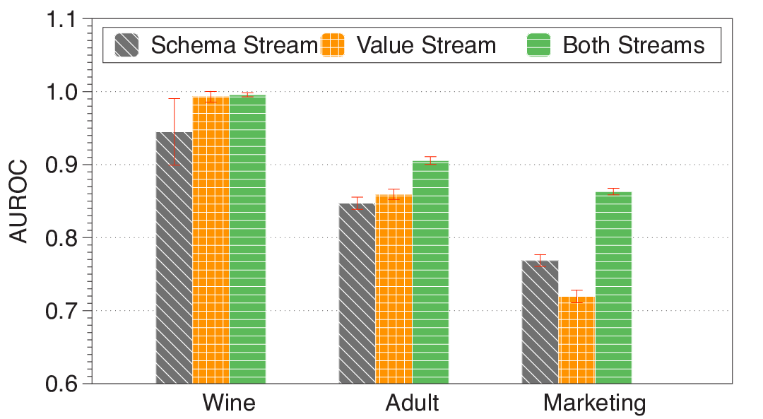
From Figure 9, we see that for Adult and Marketing, PicketNet with two streams outperforms both one-stream options. For Wine, the value stream itself works fine, but a combination of the two streams does not impair the performance of the model. Neither of the two one-stream options demonstrates obvious superiority over the other one, since there are cases that the value stream performs better than the schema stream, and cases that the opposite happens.
Effectiveness of the Early Filtering Mechanism
We validate the effectiveness of early filtering by comparing the performance of outlier detection at the early stage of PicketNet’s training to that after convergence. The results are shown in Figure 10. We use the setup from the previous micro-benchmark.
Figure 10 shows that filtering at early stages consistently outperforms filtering after convergence. The reason is that in the early stage of training, the model is less likely to overfit to the input, and therefore the reconstruction loss of the outliers differs from that of the clean samples more.

Histogram-Based Threshold Selection We validate the effectiveness of the histogram-based threshold selection strategy mentioned in Section 4.2. To better illustrate how it affects the downstream accuracy, we use Wine and HTRU2 with poisoning attacks (20% of the samples are poisoned) where corruption has a significant effect on the downstream models. For each dataset and downstream model combination, we plot the histogram of the Picket reconstruction loss in Figure 11, and select the thresholds and accordingly so that the abnormal peaks and low-density tails are filtered out. We report the downstream accuracy after filtering with this strategy (Picket-Hist) in Table 7. Same as Section 6.2, we also report the downstream accuracy under CL and NF as reference points. The results show that Picket-Hist gets very close to CL where the data is clean, and much better than NF where no filtering is applied, which verifies the effectiveness of this threshold-selection strategy.


| Dataset | Downstream Model | Picket-Hist | CL | NF |
|---|---|---|---|---|
| Wine | LR | 0.7500 | 0.7551 | 0.6846 |
| SVM | 0.7459 | 0.7530 | 0.6836 | |
| NN | 0.7133 | 0.7204 | 0.6561 | |
| HTRU2 | LR | 0.9344 | 0.9435 | 0.8810 |
| SVM | 0.9375 | 0.9435 | 0.8856 | |
| NN | 0.9207 | 0.9207 | 0.8720 |
Effectiveness of Per-Class Victim Sample Detectors We compare the performance of our per-class detectors against a unified detector and a score-based detector. The unified detector uses one single logistic regression model over the same features to distinguish between good and victim samples regardless of the downstream predictions. The score-based detector follows the logic of the training time outlier detector, i.e., it aggregates the reconstruction losses attribute-wise, and considers samples with high loss as victims. We perform the comparison on three datasets with all of the three downstream models: Wine with adversarial noise, Adult with systematic noise (Medium level) and Marketing with random noise (Medium level).
The result is shown in Table 8. Per-Class Detectors outperform the other two, which validates the effectiveness of having one detector per-class. The unified detector performs poorly because the victim samples in one class differ from those in the other statistically, in which case one class may suffer from corruption in one group of attributes, while the other class may suffer from that in another group of attributes. The score-based detector does not work well since it only has access to the noise level of the samples but does not consider the connection between corruptions and the downstream prediction.
| Dataset | Downstream Model | Per-Class Detectors | Unified Detector | Score-based Detector |
|---|---|---|---|---|
| Wine | LR | 0.8188 | 0.7023 | 0.6885 |
| SVM | 0.8287 | 0.7152 | 0.7261 | |
| NN | 0.7444 | 0.4027 | 0.6594 | |
| Adult | LR | 0.8489 | 0.6710 | 0.7197 |
| SVM | 0.8634 | 0.6983 | 0.7297 | |
| NN | 0.8336 | 0.6785 | 0.7225 | |
| Marketing | LR | 0.8553 | 0.7740 | 0.7343 |
| SVM | 0.8618 | 0.7774 | 0.7361 | |
| NN | 0.8152 | 0.7370 | 0.7174 |
Effectiveness of Mixed Artificial Noise We validate the effectiveness of our artificial noise setting (Mixed) by comparing it to the setting where the artificial noise is generated in the same way as the test time noise (Exact). The results are shown in Table 9. We use the same datasets and test time noise as the previous micro-benchmark. We find that with mixed artificial noise, the performance of Picket is comparable to the setting where the exact noise distribution is known under random (see Marketing) and systematic noise (see Adult). Under adversarial noise (see Wine), Exact is better than Mixed but the gap is not excessively large.
| Dataset | Downstream Model | Mixed | Exact |
|---|---|---|---|
| Wine | LR | 0.8197 | 0.8646 |
| SVM | 0.8291 | 0.8812 | |
| NN | 0.7442 | 0.7790 | |
| Adult | LR | 0.8501 | 0.8372 |
| SVM | 0.8643 | 0.8562 | |
| NN | 0.8336 | 0.8157 | |
| Marketing | LR | 0.8549 | 0.8544 |
| SVM | 0.8607 | 0.8592 | |
| NN | 0.8162 | 0.8120 |
6.5. Fairness of Outlier Detection
We compute the equality of opportunity between majority and minority groups to check the fairness of outlier detection. Specifically, the opportunity for each group is defined as the fraction of clean examples in that group that are kept after filtering:
where is the number of clean examples in group , and is the number of clean examples in that are not filtered out. We report the difference of opportunity , where is the majority group and is the minority. closer to indicates better fairness.
We choose two demographic datasets, Adult and Marketing, to verify the fairness of the outlier detection methods. For each dataset, we pick one sensitive attribute at a time, and divide its value domain into majority and minority groups as follows:
- (1)
Sort the values by their frequency in descending order.
- (2)
Add values in order to the majority group until it covers more than 80% of the examples.
- (3)
Add the rest of the values into the minority group.
We inject random and systematic noise of medium magnitude to 20% of the examples, filter out 20%, and report the difference of opportunity for each dataset-attribute combination in Table 10. We can see that for most of the sensitive attributes, the difference of opportunity is less than if the data are filtered by Picket. However, for certain attributes (e.g. Marketing-Marital and Marketing-Language), the difference is quite large, which shows potential risk of unfairness. The other models also show bias towards the majority group for certain attributes. We defer the improvement of fairness as a future direction to explore.
| Noise Type | Dataset-Attribute | IF | OCSVM | RVAE | Picket |
|---|---|---|---|---|---|
| Random | Marketing-Marital | -0.0469 | -0.0821 | -0.0196 | -0.1400 |
| Marketing-Age | 0.0720 | -0.0071 | 0.0019 | 0.0216 | |
| Marketing-Education | -0.0436 | -0.0521 | -0.0192 | 0.0174 | |
| Marketing-Live | -0.1131 | -0.1242 | -0.0488 | -0.0242 | |
| Marketing-Dual | -0.0226 | -0.0737 | -0.0357 | -0.0089 | |
| Marketing-Hometype | -0.0865 | -0.1581 | -0.0634 | -0.0458 | |
| Marketing-Ethnic | -0.1762 | -0.2258 | -0.0760 | -0.0610 | |
| Marketing-Language | -0.5625 | -0.4739 | -0.0753 | -0.3739 | |
| Adult-Workclass | -0.1290 | -0.0259 | -0.0277 | -0.0042 | |
| Adult-Marital-status | -0.3111 | -0.0676 | -0.0013 | -0.0706 | |
| Adult-Relationship | -0.2545 | 0.0027 | 0.0081 | -0.0188 | |
| Adult-Race | -0.4452 | -0.0326 | -0.0259 | -0.0515 | |
| Systematic | Marketing-Marital | -0.0541 | -0.1178 | -0.0418 | -0.2031 |
| Marketing-Age | 0.0902 | -0.0051 | 0.0097 | 0.0270 | |
| Marketing-Education | -0.0366 | -0.0509 | -0.0164 | 0.0142 | |
| Marketing-Live | -0.0781 | -0.1333 | -0.0640 | -0.0090 | |
| Marketing-Dual | -0.0275 | -0.0757 | -0.0224 | -0.0244 | |
| Marketing-Hometype | -0.0995 | -0.1892 | -0.1182 | -0.0528 | |
| Marketing-Ethnic | -0.1919 | -0.2465 | -0.1388 | -0.0777 | |
| Marketing-Language | -0.5981 | -0.5397 | -0.1555 | -0.4791 | |
| Adult-Workclass | -0.1819 | -0.0079 | -0.0287 | -0.0012 | |
| Adult-Marital-status | -0.3158 | -0.0690 | 0.0026 | -0.2519 | |
| Adult-Relationship | -0.2444 | -0.0148 | 0.0067 | -0.0635 | |
| Adult-Race | -0.4124 | -0.0560 | -0.0088 | -0.0719 |
6.6. Runtime and Scalability
We report the training time of PicketNet for each dataset in Table 12. The device we use is a single NVIDIA Tesla V100-PCIE GPU with 32GB memory. Note that the current runtime has not been fully optimized.
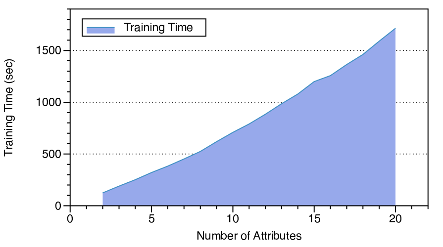
We also study the attribute-wise scalibilty of PicketNet using synthetic datasets. The datasets have a different number of attributes ranging from 2 to 20 with a increase step of one, while the other settings are the same (the dimension of and is fixed to 8). We report the training time of 100 epochs in Figure 12. The growth of the runtime is roughly quadratic as the number of attributes increases. This is expected since the dependencies between one attribute and all the others yield quadratic complexity. When the number of attributes is excessively large, we can apply simple methods like computing the correlations between attributes to split the attributes into groups, where only the attributes within the same group exhibit correlations. Then, we can apply PicketNet to learn the structure for each of the groups. We evaluate the effectiveness of this strategy on the Alarm dataset (Herskovits 1992) which contains 36 attributes and 1000 records. The functional dependencies in Alarm is known. We split the attributes into three groups based on the functional dependencies. Each group contains 12 of them. We run Picket outlier detection on the three groups independently, and then aggregate the reconstruction loss across groups. We inject random and systematic noise of medium magnitude to 20% of the records, and report the AUROC of outlier detection in Table 11. The results show that Picket provides high-quality outlier detection under the aforementioned strategy.
| Noise Type | IF | OCSVM | RVAE | Picket |
| Random | 0.8848 | 0.8835 | 0.9357 | 0.9579 |
| Systematic | 0.7410 | 0.7283 | 0.7957 | 0.7967 |
We report the inference time overhead (runtime of PicketNet loss computing and victim sample detectors) as long as the runtime of downstream prediction of each dataset in Table 13, when the data come in batches of 100. We can see that the overhead of PicketNet loss computing dominates the runtime, but it is still no more than a few seconds. As the downstream model becomes more complex, the relative overhead introduced by Picket would be reduced.
| Dataset | Wine | Adult | Restaurant | Marketing | Titanic | HTRU2 |
| Training Time (sec) | 1953 | 8256 | 3794 | 4581 | 1693 | 189 |
|---|
| Dataset | Wine | Adult | Restaurant | Marketing | Titanic | HTRU2 |
|---|---|---|---|---|---|---|
| PicketNet Loss Computing (sec) | 0.1512 | 0.4303 | 0.3003 | 0.4048 | 0.2892 | 0.0316 |
| Victim Sample Detectors (sec) | 0.0006 | 0.0009 | 0.0012 | 0.0009 | 0.0008 | 0.0004 |
| Downstream Prediction (LR) (sec) | 0.0003 | 0.0010 | 0.0016 | 0.0011 | 0.0006 | 0.0003 |
| Downstream Prediction (SVM) (sec) | 0.0003 | 0.0021 | 0.0012 | 0.0012 | 0.0006 | 0.0003 |
| Downstream Prediction (NN) (sec) | 0.0004 | 0.0021 | 0.0030 | 0.0014 | 0.0005 | 0.0004 |
7. Related Work
Data Validation Systems for ML TFX (Baylor et al. 2017; Breck et al. [n.d.]) and Deequ (Schelter et al. 2019) propose data validation modules that rely on user-defined constraints and simple anomaly detection. CleanML (Li et al. 2019) studies how the quality of training data affects the performance of downstream models. These works focus on simple constraints such as data types, value ranges, and one-column statistics and ignore the structure of the data. NaCL (Khosravi et al. 2019) and CPClean (Karlaš et al. 2020) propose algorithms to deal with missing entries, and the effect of missing entries are analyzed theoretically in (Liu et al. 2020). These works are orthogonal to ours since they only consider missing entries.
Learning Dependencies with Attention Mechanisms Attention mechanisms have been widely used in the field of natural language processing to learn the dependencies between tokens (Vaswani et al. 2017; Yang et al. 2019). Recently, AimNet (Wu et al. 2020) demonstrates that attention mechanisms are also effective in learning the dependencies between attributes in structured tabular data. AimNet employs the attention techniques to impute the missing values in tabular data and achieve state-of-the-art performance. AimNet is rather simplistic and it only captures schema-level dependencies. Furthermore, AimNet requires clean training data and does not employ any robust-training mechanism to tolerate noise.
Outlier Detection Methods Outlier detection for tabular data has been studied for years, and many rule-based methods have been proposed (Ilyas and Chu 2015; Rahm and Do 2000; Fan and Geerts 2012). Learning-based outlier detection has become popular recently and focuses on semi-supervised or unsupervised approaches. Semi-supervised methods such as the ones proposed in (Heidari et al. 2019; Xue et al. 2010; Mahdavi et al. 2019) still need human in the loop to explicitly label some data. Isolation Forest (Liu et al. 2008) and One-Class SVM (Chen et al. 2001) are simple unsupervised methods that are widely used. Autoencoder-based outlier detection methods (An and Cho 2015; Sabokrou et al. 2016; Eduardo et al. 2020) are most relevant to our work since they also rely on the reconstruction of the input, and among them RVAE (Eduardo et al. 2020) works best for mixed-type tabular data.
Adversarial Attacks and Defenses Training time attacks (Koh et al. 2018; Muñoz-González et al. 2017; Biggio et al. 2012) add poisoned samples to corrupt the target model. Filtering-based defenses (Steinhardt et al. 2017; Diakonikolas et al. 2018) remove suspicious samples during training based on training statistics. Inference time attacks (Madry et al. 2018a; Carlini and Wagner 2017; Moosavi-Dezfooli et al. 2016) add small perturbation to test samples to fool the classifier. Efforts have been made to improve the robustness of the model by training data augmentation (Goodfellow et al. 2014; Madry et al. 2018b) or making modifications to the model (Xiao et al. 2019; Pang et al. 2020; Pang et al. 2019). Those works focus on robustness from the model perspective without assessment of data quality. Hence, they are orthogonal to ours. Another group of defenses trying to detect adversarial samples at inference time are more directly related to our work. Roth et al. (Roth et al. 2019) and Hu et al. (Hu et al. 2019) add random noise to input samples and detect suspicious ones based on the changes in the logit values. Grosse et al. (Grosse et al. 2017) assume that adversarial samples have different distributions from benign samples and add another class to the classifier to detect them.
8. Conclusion
We introduced Picket, a first-of-its-kind system that safeguards against data corruptions for machine learning pipelines over tabular data either during training or deployment. To design Picket, we introduced PicketNet, a novel self-supervised deep learning model that corresponds to a Transformer network for tabular data. Picket is designed as a plugin that can increase the robustness of any machine learning pipeline.
References
- (1)
- An and Cho (2015) Jinwon An and Sungzoon Cho. 2015. Variational autoencoder based anomaly detection using reconstruction probability. Special Lecture on IE 2, 1 (2015).
- Arora et al. (2019) Sanjeev Arora, Yingyu Liang, and Tengyu Ma. 2019. A simple but tough-to-beat baseline for sentence embeddings. 5th International Conference on Learning Representations, ICLR 2017 ; Conference date: 24-04-2017 Through 26-04-2017.
- Baylor et al. (2017) Denis Baylor, Eric Breck, Heng-Tze Cheng, Noah Fiedel, Chuan Yu Foo, Zakaria Haque, Salem Haykal, Mustafa Ispir, Vihan Jain, Levent Koc, Chiu Yuen Koo, Lukasz Lew, Clemens Mewald, Akshay Naresh Modi, Neoklis Polyzotis, Sukriti Ramesh, Sudip Roy, Steven Euijong Whang, Martin Wicke, Jarek Wilkiewicz, Xin Zhang, and Martin Zinkevich. 2017. TFX: A TensorFlow-Based Production-Scale Machine Learning Platform. In Proceedings of the 23rd ACM SIGKDD International Conference on Knowledge Discovery and Data Mining (Halifax, NS, Canada) (KDD ’17). Association for Computing Machinery, New York, NY, USA, 1387–1395. https://doi.org/10.1145/3097983.3098021
- Biggio et al. (2012) Battista Biggio, Blaine Nelson, and Pavel Laskov. 2012. Poisoning Attacks against Support Vector Machines. In Proceedings of the 29th International Coference on International Conference on Machine Learning (Edinburgh, Scotland) (ICML’12). Omnipress, Madison, WI, USA, 1467–1474.
- Bojanowski et al. (2017) Piotr Bojanowski, Edouard Grave, Armand Joulin, and Tomas Mikolov. 2017. Enriching Word Vectors with Subword Information. Transactions of the Association for Computational Linguistics 5 (2017), 135–146.
- Breck et al. ([n.d.]) Eric Breck, Neoklis Polyzotis, Sudip Roy, Steven Euijong Whang, and Martin Zinkevich. [n.d.]. Data validation for machine learning. In MLSys-19.
- Carlini and Wagner (2017) Nicholas Carlini and David Wagner. 2017. Towards evaluating the robustness of neural networks. In 2017 ieee symposium on security and privacy (sp). IEEE, 39–57.
- Chen et al. (2001) Yunqiang Chen, Xiang Sean Zhou, and Thomas S Huang. 2001. One-class SVM for learning in image retrieval. In Proceedings 2001 International Conference on Image Processing (Cat. No. 01CH37205), Vol. 1. IEEE, 34–37.
- Devlin et al. (2018) Jacob Devlin, Ming-Wei Chang, Kenton Lee, and Kristina Toutanova. 2018. BERT: Pre-training of Deep Bidirectional Transformers for Language Understanding. arXiv preprint arXiv:1810.04805 (2018).
- Diakonikolas et al. (2017) Ilias Diakonikolas, Gautam Kamath, Daniel M Kane, Jerry Li, Ankur Moitra, and Alistair Stewart. 2017. Being robust (in high dimensions) can be practical. In Proceedings of the 34th International Conference on Machine Learning-Volume 70. JMLR. org, 999–1008.
- Diakonikolas et al. (2018) Ilias Diakonikolas, Gautam Kamath, Daniel M Kane, Jerry Li, Jacob Steinhardt, and Alistair Stewart. 2018. Sever: A robust meta-algorithm for stochastic optimization. arXiv preprint arXiv:1803.02815 (2018).
- Dietterich (1998) Thomas G Dietterich. 1998. Approximate statistical tests for comparing supervised classification learning algorithms. Neural computation 10, 7 (1998), 1895–1923.
- Dua and Graff (2017) Dheeru Dua and Casey Graff. 2017. UCI Machine Learning Repository. http://archive.ics.uci.edu/ml
- Eduardo et al. (2020) Simão Eduardo, Alfredo Nazábal, Christopher K. I. Williams, and Charles Sutton. 2020. Robust Variational Autoencoders for Outlier Detection in Mixed-Type Data. In The 23rd International Conference on Artificial Intelligence and Statistics.
- Fan and Geerts (2012) Wenfei Fan and Floris Geerts. 2012. Foundations of data quality management. Morgan & Claypool Publishers.
- Goodfellow et al. (2014) Ian J Goodfellow, Jonathon Shlens, and Christian Szegedy. 2014. Explaining and harnessing adversarial examples. arXiv preprint arXiv:1412.6572 (2014).
- Goodfellow et al. (2015) Ian J. Goodfellow, Jonathon Shlens, and Christian Szegedy. 2015. Explaining and Harnessing Adversarial Examples. CoRR abs/1412.6572 (2015).
- Grosse et al. (2017) Kathrin Grosse, Praveen Manoharan, Nicolas Papernot, Michael Backes, and Patrick McDaniel. 2017. On the (statistical) detection of adversarial examples. arXiv preprint arXiv:1702.06280 (2017).
- Guo et al. (2017) Chuan Guo, Geoff Pleiss, Yu Sun, and Kilian Q Weinberger. 2017. On calibration of modern neural networks. In Proceedings of the 34th International Conference on Machine Learning-Volume 70. JMLR. org, 1321–1330.
- Heidari et al. (2019) Alireza Heidari, Joshua McGrath, Ihab F Ilyas, and Theodoros Rekatsinas. 2019. Holodetect: Few-shot learning for error detection. In Proceedings of the 2019 International Conference on Management of Data. 829–846.
- Herskovits (1992) Edward Herskovits. 1992. Computer-Based Probabilistic-Network Construction. Ph.D. Dissertation. Stanford, CA, USA. UMI Order No. GAX92-05646.
- Hu et al. (2019) Shengyuan Hu, Tao Yu, Chuan Guo, Wei-Lun Chao, and Kilian Q Weinberger. 2019. A New Defense Against Adversarial Images: Turning a Weakness into a Strength. In Advances in Neural Information Processing Systems. 1633–1644.
- Ilyas and Chu (2015) Ihab F Ilyas and Xu Chu. 2015. Trends in cleaning relational data: Consistency and deduplication. Foundations and Trends in Databases 5, 4 (2015), 281–393.
- Karlaš et al. (2020) Bojan Karlaš, Peng Li, Renzhi Wu, Nezihe Merve Gürel, Xu Chu, Wentao Wu, and Ce Zhang. 2020. Nearest Neighbor Classifiers over Incomplete Information: From Certain Answers to Certain Predictions. arXiv:2005.05117 [cs.LG]
- Khosravi et al. (2019) Pasha Khosravi, Yitao Liang, YooJung Choi, and Guy Van den Broeck. 2019. What to Expect of Classifiers? Reasoning about Logistic Regression with Missing Features. In Proceedings of the Twenty-Eighth International Joint Conference on Artificial Intelligence, IJCAI-19. International Joint Conferences on Artificial Intelligence Organization, 2716–2724. https://doi.org/10.24963/ijcai.2019/377
- Kingma and Ba (2014) Diederik P Kingma and Jimmy Ba. 2014. Adam: A method for stochastic optimization. arXiv preprint arXiv:1412.6980 (2014).
- Koh et al. (2018) Pang Wei Koh, Jacob Steinhardt, and Percy Liang. 2018. Stronger data poisoning attacks break data sanitization defenses. arXiv preprint arXiv:1811.00741 (2018).
- Li et al. (2019) Peng Li, Xi Rao, Jennifer Blase, Yue Zhang, Xu Chu, and Ce Zhang. 2019. CleanML: A Benchmark for Joint Data Cleaning and Machine Learning [Experiments and Analysis]. arXiv preprint arXiv:1904.09483 (2019).
- Liu et al. (2008) Fei Tony Liu, Kai Ming Ting, and Zhi-Hua Zhou. 2008. Isolation forest. In 2008 Eighth IEEE International Conference on Data Mining. IEEE, 413–422.
- Liu et al. (2020) Zifan Liu, Jongho Park, Nils Palumbo, Theodoros Rekatsinas, and Christos Tzamos. 2020. Robust Mean Estimation under Coordinate-level Corruption. arXiv:2002.04137 [cs.LG]
- Madry et al. (2018a) Aleksander Madry, Aleksandar Makelov, Ludwig Schmidt, Dimitris Tsipras, and Adrian Vladu. 2018a. Towards Deep Learning Models Resistant to Adversarial Attacks. In International Conference on Learning Representations. https://openreview.net/forum?id=rJzIBfZAb
- Madry et al. (2018b) Aleksander Madry, Aleksandar Makelov, Ludwig Schmidt, Dimitris Tsipras, and Adrian Vladu. 2018b. Towards Deep Learning Models Resistant to Adversarial Attacks. In International Conference on Learning Representations. https://openreview.net/forum?id=rJzIBfZAb
- Mahdavi et al. (2019) Mohammad Mahdavi, Ziawasch Abedjan, Raul Castro Fernandez, Samuel Madden, Mourad Ouzzani, Michael Stonebraker, and Nan Tang. 2019. Raha: A Configuration-Free Error Detection System. In Proceedings of the 2019 International Conference on Management of Data (Amsterdam, Netherlands) (SIGMOD ’19). Association for Computing Machinery, New York, NY, USA, 865–882. https://doi.org/10.1145/3299869.3324956
- Moosavi-Dezfooli et al. (2016) Seyed-Mohsen Moosavi-Dezfooli, Alhussein Fawzi, and Pascal Frossard. 2016. Deepfool: a simple and accurate method to fool deep neural networks. In Proceedings of the IEEE conference on computer vision and pattern recognition. 2574–2582.
- Muñoz-González et al. (2017) Luis Muñoz-González, Battista Biggio, Ambra Demontis, Andrea Paudice, Vasin Wongrassamee, Emil C Lupu, and Fabio Roli. 2017. Towards poisoning of deep learning algorithms with back-gradient optimization. In Proceedings of the 10th ACM Workshop on Artificial Intelligence and Security. 27–38.
- Nicolae et al. (2018) Maria-Irina Nicolae, Mathieu Sinn, Minh Ngoc Tran, Beat Buesser, Ambrish Rawat, Martin Wistuba, Valentina Zantedeschi, Nathalie Baracaldo, Bryant Chen, Heiko Ludwig, Ian Molloy, and Ben Edwards. 2018. Adversarial Robustness Toolbox v1.2.0. CoRR 1807.01069 (2018). https://arxiv.org/pdf/1807.01069
- Pang et al. (2020) Tianyu Pang, Kun Xu, Yinpeng Dong, Chao Du, Ning Chen, and Jun Zhu. 2020. Rethinking Softmax Cross-Entropy Loss for Adversarial Robustness. In International Conference on Learning Representations. https://openreview.net/forum?id=Byg9A24tvB
- Pang et al. (2019) Tianyu Pang, Kun Xu, Chao Du, Ning Chen, and Jun Zhu. 2019. Improving adversarial robustness via promoting ensemble diversity. arXiv preprint arXiv:1901.08846 (2019).
- Rahm and Do (2000) Erhard Rahm and Hong Hai Do. 2000. Data cleaning: Problems and current approaches. IEEE Data Eng. Bull. 23, 4 (2000), 3–13.
- Roth et al. (2019) Kevin Roth, Yannic Kilcher, and Thomas Hofmann. 2019. The Odds are Odd: A Statistical Test for Detecting Adversarial Examples. In Proceedings of the 36th International Conference on Machine Learning, ICML 2019, 9-15 June 2019, Long Beach, California, USA (Proceedings of Machine Learning Research), Kamalika Chaudhuri and Ruslan Salakhutdinov (Eds.), Vol. 97. PMLR, 5498–5507. http://proceedings.mlr.press/v97/roth19a.html
- Sabokrou et al. (2016) Mohammad Sabokrou, Mahmood Fathy, and Mojtaba Hoseini. 2016. Video anomaly detection and localisation based on the sparsity and reconstruction error of auto-encoder. Electronics Letters 52, 13 (2016), 1122–1124.
- Schelter et al. (2019) Sebastian Schelter, Felix Biessmann, Dustin Lange, Tammo Rukat, Phillipp Schmidt, Stephan Seufert, Pierre Brunelle, and Andrey Taptunov. 2019. Unit Testing Data with Deequ. In Proceedings of the 2019 International Conference on Management of Data (Amsterdam, Netherlands) (SIGMOD ’19). Association for Computing Machinery, New York, NY, USA, 1993–1996. https://doi.org/10.1145/3299869.3320210
- Simonyan and Zisserman (2014) Karen Simonyan and Andrew Zisserman. 2014. Two-stream convolutional networks for action recognition in videos. In Advances in neural information processing systems. 568–576.
- Steinhardt et al. (2017) Jacob Steinhardt, Pang Wei W Koh, and Percy S Liang. 2017. Certified defenses for data poisoning attacks. In Advances in neural information processing systems. 3517–3529.
- Su et al. (2020) Weijie Su, Xizhou Zhu, Yue Cao, Bin Li, Lewei Lu, Furu Wei, and Jifeng Dai. 2020. VL-BERT: Pre-training of Generic Visual-Linguistic Representations. In International Conference on Learning Representations. https://openreview.net/forum?id=SygXPaEYvH
- Vaswani et al. (2017) Ashish Vaswani, Noam Shazeer, Niki Parmar, Jakob Uszkoreit, Llion Jones, Aidan N Gomez, Łukasz Kaiser, and Illia Polosukhin. 2017. Attention is all you need. In Advances in neural information processing systems. 5998–6008.
- Wu et al. (2020) Richard Wu, Aoqian Zhang, Ihab F Ilyas, and Theodoros Rekatsinas. 2020. Attention-based Learning for Missing Data Imputation in HoloClean. Proceedings of Machine Learning and Systems (2020), 307–325.
- Xiao et al. (2019) Chang Xiao, Peilin Zhong, and Changxi Zheng. 2019. Resisting Adversarial Attacks by -Winners-Take-All. arXiv preprint arXiv:1905.10510 (2019).
- Xue et al. (2010) Zhenxia Xue, Youlin Shang, and Aifen Feng. 2010. Semi-supervised outlier detection based on fuzzy rough C-means clustering. Mathematics and Computers in simulation 80, 9 (2010), 1911–1921.
- Yang et al. (2019) Zhilin Yang, Zihang Dai, Yiming Yang, Jaime Carbonell, Russ R Salakhutdinov, and Quoc V Le. 2019. Xlnet: Generalized autoregressive pretraining for language understanding. In Advances in neural information processing systems. 5754–5764.
Appendix A Appendix
A.1. Hyper-parameters of PicketNet
PicketNet is not sensitive to hyper-parameters in most cases. The default hyper-parameters we use in the experiments is shown in Table 14. For purely numerical datasets, we reduce the dimension of and to 8, and for HTRU2, we reduce the number of self-attention layers to 1. In the other datasets, we always use the default hyper-parameters. We use the Adam optimizer (Kingma and Ba 2014) with , and for training. The learning rate , where is the dimension of and , is the index of the training step. increases in the first few steps and then decreases. Typically, PicketNet takes 100 to 500 epochs to converge, depending on the datasets.
| Hyper-Parameter | Value |
| Number of Self-Attention Layers | 6 |
| Number of Attention Heads | 2 |
| Dimension of and | 64 |
| Number of Hidden Layers in Each Feedforward Network | 1 |
| Dimension of the Hidden Layers in Feedforward Networks | 64 |
| Dropout | 0.1 |
| Size of the Negative Sample Set | 4 |
| Warm-up Epochs for Loss-Based Filtering | 50 |
| Loss Recording Epochs | 20 |
A.2. Outlier Detection on Synthetic Data
We evaluate the performance of outlier detection on synthetic datasets to understand the effects of several aspects about the data and noise, including the strength of structure, data dimension, noise level and magnitude of extreme outliers. Here the term structure means dependencies or correlations between attributes.
We generate synthetic datasets as follows. Each synthetic data point is generated by , where and . Each entry of is sampled from the standard Gaussian distribution, and each entry of is sampled uniformly from to . Unless otherwise specified, we inject random noise with and to 20% of the samples by default.
Effect of Structure By performing outlier detection over synthetic datasets that exhibit different strength of structure, we show that the advantage of Picket over the other outlier detection methods is its ability to capture the structure of the data. We fix and vary to change the strength of structure. Smaller indicates stronger structure and more redundancy across attributes. The results are shown in Figure 13. Picket performs better when the structure is strong, while the performance of the other methods is not affected by the strength of structure, which indicates that Picket is able to capture the structure of the data and benefit from it.
Effect of Data Dimension We vary the the data dimension to study how it affects the performance. The hidden dimension is set to so that the attributes are independent. The results are shown in Figure 14. The performance of all methods increases as the data dimension gets larger. The reason is that there are more corrupted cells in corrupted samples when the dimension increases, making them easier to be detected. Note that RVAE performs quite well in this setting, which is not surprising since it is built exactly on the assumption that the data come from Gaussian distributions.
Effect of Noise Level We study the effect of noise level, including the fraction of corrupted samples, the fraction of corrupted cells in corrupted samples () and the magnitude of the random noise (). Each time we vary one of the factors and fix the others. The data dimension is fixed to , and is fixed to . As is shown in Figure 15, when we vary the fraction of corrupted samples, the performance of all methods keeps stable. Figure 16 and 17 show that the performance of all methods increases as we increase the fraction of corrupted cells in corrupted samples or the magnitude of the random noise. These results show that the corruption level of the corrupted samples have a more significant effect on the outlier detection performance than the fraction of corrupted samples.
Effect of Extreme Outliers We study how the models behave under extreme outliers with different magnitude. We corrupt 20% of the samples, and among those samples 20% of the cells are multiplied by a scaling factor. We vary the value of the scaling factor and report the detection performance in Figure 18. As the scaling factor gets larger, the performance of all methods increases. This is expected since more extreme values deviate more from the normal distribution.


A.3. Outlier Detection with Cross-Validation
We evaluate the ability to detect outliers for unseen data during training using cross-validation. We use 5 iterations of 2-fold cross-validation with a modified t-test recommended by Dietterich and Thomas (Dietterich 1998). Specifically, in each iteration, we randomly split the dataset into two folds. Then we use one fold to train the outlier detection models, and the other to validate their performance. The results are reported in Table 15. The results shows that Picket achieves the best performance among the examined methods on all dataset-noise combinations for unseen data at training time. In some cases, Picket is significantly better than all competing methods.
| Dataset | Noise Type | IF | OCSVM | RVAE | Picket |
|---|---|---|---|---|---|
| Wine | Random-Medium | 0.8876 | 0.8886 | 0.9170 | 0.9252 |
| Systematic-Medium | 0.9537 | 0.8971 | 0.9123 | 0.9669 | |
| Poison-LR | 0.9756 | 0.9054 | 0.9061 | 0.9781 | |
| Poison-SVM | 0.9761 | 0.9047 | 0.9025 | 0.9787 | |
| Poison-NN | 0.9877 | 0.8696 | 0.9356 | 0.9921 | |
| Adult | Random-Medium | 0.7800 | 0.8260 | 0.9019 | 0.9240 |
| Systematic-Medium | 0.8048 | 0.8217 | 0.8530 | 0.9180 | |
| Restaurant | Random-Medium | 0.4814 | 0.4431 | 0.6985 | 0.9281 |
| Systematic-Medium | 0.4805 | 0.4449 | 0.6596 | 0.8778 | |
| Real* | 0.5514 | 0.5116 | 0.4558 | 0.8978 | |
| Marketing | Random-Medium | 0.7539 | 0.7804 | 0.8688 | 0.8646 |
| Systematic-Medium | 0.6746 | 0.6632 | 0.7787 | 0.7810 | |
| Titanic | Random-Medium | 0.6014 | 0.6933 | 0.5819 | 0.7709 |
| Systematic-Medium | 0.5811 | 0.7037 | 0.5557 | 0.7691 | |
| Real | 0.5851 | 0.6472 | 0.5000 | 0.7314 | |
| Food | Real | 0.5094 | 0.5210 | 0.5180 | 0.5506 |
- •
*Real is short for common errors in the real world.
A.4. Performance of Training Time Outlier Detection under Different Fraction of Corrupted Samples
We vary the fraction of corrupted samples, and report the corresponding AUROC of training time outlier detection in Figure 19. The datasets we use are Wine with poisoning attack on NN, Adult with systematic noise, and Marketing with random noise. The random and systematic noise is in the Medium level.
From the results we can see that the detection performance could either increase or decrease as the fraction of corrupted samples grows, depending on the type of noise and detection method. One one hand, the outliers are easier to detect when they form a larger cluster; one the other hand, more corrupted samples may mislead the learning of the clean distribution. Nevertheless, Picket keeps a relatively consistent performance with either large or small fraction of corrupted samples, while other methods may have a large gap when the fraction varies.

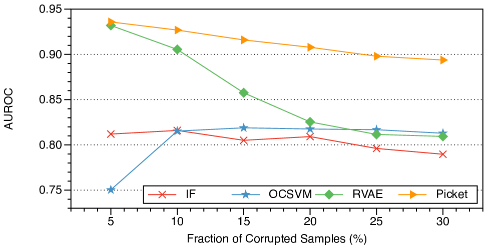

A.5. Performance of Training Time Outlier Detection under Low/High Level Random/Systematic Noise
We depict the AUROC of training time outlier detection under low/high level random/systematic noise in Figure 20, 21, 22, 23, when 20% of the samples are corrupted. The observation is quite similar to the case of medium level noise. The performance of Picket is quite good and consistent across different datasets and noise settings. RF and OCSVM perform poorly on the datasets that contain textual attributes. RVAE is competitive in some cases but fails in the others. Note that low level noise is much harder to detect than high level noise. The reason is that samples with high level noise tend to deviate a lot from the clean distribution, while samples with low level noise look quite similar to the clean ones and may not be detectable in some cases. However, low level noise will not affect the downstream model as much as high level noise, unless it is adversarially crafted.


A.6. Accuracy of Downstream Models under Random/Systematic Noise with Different Filtering Methods
We also study how the accuracy of the downstream models changes when we apply different filtering methods under random and systematic noise. We first focus on random noise. The results are shown in Tables 16, 17, 18. As expected, in the presence of random noise, the performance of the downstream models drops in some cases and remains roughly the same in the other cases if we look at CL and NF. In the cases when the downstream accuracy drops, we can see that filtering helps most of the time.
If we compare the performance of Picket and NF in Table 17 for Neural Networks, we see that for Adult, Titanic, and Restaurant Picket exhibits slightly worse test accuracy. These results are attributed to the selected thresholds for filtering in Picket (see Section 5). In Figure 24, we show the test accuracy of the downstream neural network for different levels of the Picket threshold. We can see that for some datasets, random noise serves as regularization and improves the performance of the downstream model. Therefore, we need to tune the threshold to achieve the best performance.
| Dataset | DM* | IF | OCSVM | RVAE | Picket | CL | NF |
|---|---|---|---|---|---|---|---|
| Wine | LR | 0.7429 | 0.7435 | 0.7427 | 0.7429 | 0.7457 | 0.7443 |
| SVM | 0.7447 | 0.7437 | 0.7486 | 0.7465 | 0.7465 | 0.7453 | |
| NN | 0.7857 | 0.7800 | 0.7849 | 0.7941 | 0.8051 | 0.7922 | |
| Adult | LR | 0.8207 | 0.8211 | 0.8127 | 0.8233 | 0.8240 | 0.8190 |
| SVM | 0.8181 | 0.8196 | 0.8075 | 0.8212 | 0.8238 | 0.8187 | |
| NN | 0.7818 | 0.7800 | 0.7803 | 0.7816 | 0.7909 | 0.7836 | |
| Restaurant | LR | 0.7318 | 0.7347 | 0.7361 | 0.7352 | 0.7375 | 0.7378 |
| SVM | 0.6922 | 0.7078 | 0.7123 | 0.6972 | 0.7116 | 0.7060 | |
| NN | 0.7128 | 0.6982 | 0.7099 | 0.7135 | 0.7306 | 0.7182 | |
| Marketing | LR | 0.7622 | 0.7661 | 0.7642 | 0.7663 | 0.7672 | 0.7691 |
| SVM | 0.7649 | 0.7668 | 0.7655 | 0.7678 | 0.7681 | 0.7708 | |
| NN | 0.7362 | 0.7282 | 0.7302 | 0.7265 | 0.7261 | 0.7300 | |
| Titanic | LR | 0.7810 | 0.7777 | 0.7832 | 0.7844 | 0.7877 | 0.7821 |
| SVM | 0.7799 | 0.7866 | 0.7788 | 0.7877 | 0.7888 | 0.7888 | |
| NN | 0.7654 | 0.7542 | 0.7531 | 0.7654 | 0.7743 | 0.7709 |
- •
*DM = Downstream Model.
| Dataset | DM* | IF | OCSVM | RVAE | Picket | CL | NF |
|---|---|---|---|---|---|---|---|
| Wine | LR | 0.7410 | 0.7396 | 0.7410 | 0.7398 | 0.7457 | 0.7280 |
| SVM | 0.7441 | 0.7457 | 0.7443 | 0.7431 | 0.7467 | 0.7259 | |
| NN | 0.7743 | 0.7776 | 0.7816 | 0.7776 | 0.7973 | 0.7761 | |
| Adult | LR | 0.8140 | 0.8220 | 0.8233 | 0.8224 | 0.8240 | 0.8111 |
| SVM | 0.8109 | 0.8200 | 0.8219 | 0.8207 | 0.8238 | 0.8082 | |
| NN | 0.7856 | 0.7795 | 0.7830 | 0.7850 | 0.7934 | 0.7883 | |
| Restaurant | LR | 0.7342 | 0.7321 | 0.7313 | 0.7366 | 0.7375 | 0.7349 |
| SVM | 0.7111 | 0.7083 | 0.6898 | 0.6858 | 0.7185 | 0.6872 | |
| NN | 0.7059 | 0.7064 | 0.7062 | 0.7157 | 0.7298 | 0.7210 | |
| Marketing | LR | 0.7645 | 0.7624 | 0.7642 | 0.7656 | 0.7672 | 0.7665 |
| SVM | 0.7654 | 0.7639 | 0.7654 | 0.7665 | 0.7681 | 0.7669 | |
| NN | 0.7267 | 0.7360 | 0.7301 | 0.7344 | 0.7311 | 0.7310 | |
| Titanic | LR | 0.7799 | 0.7821 | 0.7777 | 0.7877 | 0.7877 | 0.7754 |
| SVM | 0.7810 | 0.7765 | 0.7788 | 0.7933 | 0.7888 | 0.7821 | |
| NN | 0.7575 | 0.7665 | 0.7408 | 0.7765 | 0.7944 | 0.7844 |
- •
*DM = Downstream Model.
| Dataset | DM* | IF | OCSVM | RVAE | Picket | CL | NF |
|---|---|---|---|---|---|---|---|
| Wine | LR | 0.7410 | 0.7406 | 0.7398 | 0.7418 | 0.7457 | 0.6861 |
| SVM | 0.7441 | 0.7414 | 0.7427 | 0.7453 | 0.7469 | 0.6806 | |
| NN | 0.7865 | 0.7839 | 0.7896 | 0.7806 | 0.7941 | 0.7780 | |
| Adult | LR | 0.8047 | 0.8196 | 0.8218 | 0.8224 | 0.8240 | 0.8002 |
| SVM | 0.8024 | 0.8196 | 0.8207 | 0.8205 | 0.8238 | 0.7971 | |
| NN | 0.7853 | 0.7763 | 0.7867 | 0.7861 | 0.7982 | 0.7863 | |
| Restaurant | LR | 0.7380 | 0.7369 | 0.7335 | 0.7327 | 0.7375 | 0.7416 |
| SVM | 0.7161 | 0.7060 | 0.7154 | 0.7126 | 0.7053 | 0.6872 | |
| NN | 0.7147 | 0.7172 | 0.7155 | 0.7206 | 0.7251 | 0.7247 | |
| Marketing | LR | 0.7653 | 0.7649 | 0.7641 | 0.7668 | 0.7672 | 0.7671 |
| SVM | 0.7660 | 0.7660 | 0.7659 | 0.7699 | 0.7681 | 0.7686 | |
| NN | 0.7255 | 0.7265 | 0.7284 | 0.7271 | 0.7245 | 0.7295 | |
| Titanic | LR | 0.7877 | 0.7777 | 0.7799 | 0.7799 | 0.7877 | 0.7877 |
| SVM | 0.7922 | 0.7810 | 0.7855 | 0.7799 | 0.7888 | 0.7844 | |
| NN | 0.7609 | 0.7687 | 0.7709 | 0.7765 | 0.7866 | 0.7832 |
- •
*DM = Downstream Model.

We then turn our attention to systematic noise. The results are shown in Table 19, 20, 21. Picket performs the best in most cases, but still the numbers are quite close. Under common errors in the real world, CL and NF are also quite close, and filtering does not help.
| Dataset | DM* | IF | OCSVM | RVAE | Picket | CL | NF |
|---|---|---|---|---|---|---|---|
| Wine | LR | 0.7418 | 0.7424 | 0.7478 | 0.7473 | 0.7457 | 0.7408 |
| SVM | 0.7422 | 0.7453 | 0.7498 | 0.7492 | 0.7473 | 0.7484 | |
| NN | 0.7876 | 0.7890 | 0.7882 | 0.7976 | 0.8045 | 0.7939 | |
| Adult | LR | 0.8224 | 0.8205 | 0.8209 | 0.8189 | 0.8240 | 0.8200 |
| SVM | 0.8203 | 0.8196 | 0.8165 | 0.8170 | 0.8238 | 0.8186 | |
| NN | 0.7816 | 0.7746 | 0.7748 | 0.7779 | 0.7955 | 0.7815 | |
| Restaurant | LR | 0.7336 | 0.7339 | 0.7359 | 0.7336 | 0.7375 | 0.7356 |
| SVM | 0.7063 | 0.6863 | 0.7035 | 0.7082 | 0.7108 | 0.7047 | |
| NN | 0.7113 | 0.7072 | 0.7079 | 0.7160 | 0.7301 | 0.7201 | |
| Marketing | LR | 0.7639 | 0.7630 | 0.7616 | 0.7644 | 0.7672 | 0.7668 |
| SVM | 0.7658 | 0.7634 | 0.7614 | 0.7683 | 0.7681 | 0.7676 | |
| NN | 0.7316 | 0.7305 | 0.7329 | 0.7312 | 0.7324 | 0.7325 | |
| Titanic | LR | 0.7866 | 0.7888 | 0.7799 | 0.7989 | 0.7877 | 0.7821 |
| SVM | 0.7899 | 0.7866 | 0.7754 | 0.8022 | 0.7888 | 0.7911 | |
| NN | 0.7575 | 0.7520 | 0.7564 | 0.7598 | 0.7944 | 0.8011 |
- •
*DM = Downstream Model.
| Dataset | DM* | IF | OCSVM | RVAE | Picket | CL | NF |
|---|---|---|---|---|---|---|---|
| Wine | LR | 0.7414 | 0.7388 | 0.7435 | 0.7445 | 0.7457 | 0.7316 |
| SVM | 0.7441 | 0.7384 | 0.7459 | 0.7463 | 0.7461 | 0.7316 | |
| NN | 0.7959 | 0.7933 | 0.7918 | 0.7953 | 0.8000 | 0.7855 | |
| Adult | LR | 0.8136 | 0.8156 | 0.8207 | 0.8171 | 0.8240 | 0.8098 |
| SVM | 0.8103 | 0.8142 | 0.8178 | 0.8159 | 0.8238 | 0.8080 | |
| NN | 0.7822 | 0.7839 | 0.7843 | 0.7837 | 0.7931 | 0.7869 | |
| Restaurant | LR | 0.7305 | 0.7315 | 0.7351 | 0.7383 | 0.7375 | 0.7372 |
| SVM | 0.7070 | 0.7008 | 0.7107 | 0.7077 | 0.7136 | 0.6964 | |
| NN | 0.7198 | 0.7154 | 0.7175 | 0.7228 | 0.7346 | 0.7215 | |
| Marketing | LR | 0.7642 | 0.7640 | 0.7660 | 0.7673 | 0.7672 | 0.7664 |
| SVM | 0.7670 | 0.7658 | 0.7655 | 0.7686 | 0.7681 | 0.7686 | |
| NN | 0.7272 | 0.7311 | 0.7251 | 0.7281 | 0.7277 | 0.7295 | |
| Titanic | LR | 0.7877 | 0.7821 | 0.7799 | 0.7866 | 0.7877 | 0.7877 |
| SVM | 0.7922 | 0.7777 | 0.7821 | 0.8022 | 0.7888 | 0.7911 | |
| NN | 0.7464 | 0.7508 | 0.7464 | 0.7553 | 0.7866 | 0.7777 |
- •
*DM = Downstream Model.
| Dataset | DM* | IF | OCSVM | RVAE | Picket | CL | NF |
|---|---|---|---|---|---|---|---|
| Wine | LR | 0.7437 | 0.7359 | 0.7443 | 0.7447 | 0.7457 | 0.7100 |
| SVM | 0.7457 | 0.7365 | 0.7476 | 0.7455 | 0.7467 | 0.7041 | |
| NN | 0.7961 | 0.7961 | 0.7990 | 0.8008 | 0.7992 | 0.8031 | |
| Adult | LR | 0.8071 | 0.8055 | 0.8193 | 0.8079 | 0.8240 | 0.8011 |
| SVM | 0.8039 | 0.8038 | 0.8175 | 0.8060 | 0.8238 | 0.8002 | |
| NN | 0.7843 | 0.7800 | 0.7834 | 0.7822 | 0.7961 | 0.7885 | |
| Restaurant | LR | 0.7329 | 0.7332 | 0.7346 | 0.7371 | 0.7375 | 0.7361 |
| SVM | 0.7155 | 0.7051 | 0.7041 | 0.7187 | 0.6726 | 0.6925 | |
| NN | 0.7100 | 0.7032 | 0.7132 | 0.7111 | 0.7232 | 0.7124 | |
| Marketing | LR | 0.7653 | 0.7655 | 0.7638 | 0.7636 | 0.7672 | 0.7656 |
| SVM | 0.7656 | 0.7661 | 0.7646 | 0.7640 | 0.7681 | 0.7678 | |
| NN | 0.7292 | 0.7304 | 0.7256 | 0.7258 | 0.7303 | 0.7294 | |
| Titanic | LR | 0.7777 | 0.7788 | 0.7821 | 0.7799 | 0.7877 | 0.7877 |
| SVM | 0.7799 | 0.7855 | 0.7855 | 0.7799 | 0.7888 | 0.7866 | |
| NN | 0.7553 | 0.7598 | 0.7654 | 0.7441 | 0.7855 | 0.7832 |
- •
*DM = Downstream Model.
| Dataset | DM* | IF | OCSVM | RVAE | Picket | CL | NF |
|---|---|---|---|---|---|---|---|
| Restaurant | LR | 0.7388 | 0.7351 | 0.7328 | 0.7351 | 0.7404 | 0.7395 |
| SVM | 0.7028 | 0.6937 | 0.6922 | 0.7072 | 0.6959 | 0.7112 | |
| NN | 0.7187 | 0.7176 | 0.7204 | 0.7137 | 0.7118 | 0.7215 | |
| Titanic | LR | 0.7464 | 0.7497 | 0.7732 | 0.7475 | 0.7799 | 0.7609 |
| SVM | 0.7363 | 0.7363 | 0.7609 | 0.7520 | 0.7542 | 0.7598 | |
| NN | 0.7274 | 0.7251 | 0.7285 | 0.7318 | 0.7095 | 0.7207 | |
| Food | LR | 0.6628 | 0.6960 | 0.6917 | 0.6978 | 0.7163 | 0.6868 |
| SVM | 0.6529 | 0.6849 | 0.6720 | 0.6794 | 0.7095 | 0.7108 | |
| NN | 0.6505 | 0.6443 | 0.6431 | 0.6560 | 0.6609 | 0.6597 |
- •
*DM = Downstream Model.
A.7. Test Time Victim Sample Detection under Low/High Level Random/Systematic Noise
In Table 23, 24, 25, 26, we show the F1 scores of victim sample detection under low/high level random/systematic noise. The artificial noise setting is the same as described in Section 6.3. We can see that Picket outperforms all the other methods in most cases. MWOC performs quite well for the Wine dataset, but it fails completely under high random noise (the F1 score is 0.33). Similar to the case of medium noise, we observe that the reconstruction loss from PicketNet provides extra signals that improve the detection of victim samples (see the comparison between RF and Picket).
| Dataset | DM* | RF | RVAE | RVAE+ | CCS | KNN | TOAO | MWOC | Picket |
|---|---|---|---|---|---|---|---|---|---|
| Wine | LR | 0.7408 | 0.6910 | 0.7523 | 0.6667 | 0.6626 | 0.4971 | 0.8084 | 0.7824 |
| SVM | 0.7440 | 0.6918 | 0.7558 | 0.6667 | 0.6638 | 0.6016 | 0.8004 | 0.7828 | |
| NN | 0.6882 | 0.6318 | 0.6456 | 0.6770 | 0.6656 | 0.5231 | 0.7202 | 0.6713 | |
| Adult | LR | 0.8393 | 0.6563 | 0.8486 | 0.6696 | 0.7834 | 0.1968 | 0.7902 | 0.8685 |
| SVM | 0.8456 | 0.6743 | 0.8535 | 0.6691 | 0.8131 | 0.4602 | 0.7114 | 0.8714 | |
| NN | 0.8017 | 0.5429 | 0.8052 | 0.6635 | 0.6806 | 0.1900 | 0.7965 | 0.8267 | |
| Restaurant | LR | 0.7870 | –# | – | 0.7586 | 0.6702 | 0.6441 | 0.7649 | 0.8328 |
| SVM | 0.6370 | – | – | 0.6895 | 0.6351 | 0.6634 | 0.5538 | 0.7123 | |
| NN | 0.7609 | – | – | 0.7066 | 0.6643 | 0.6071 | 0.7075 | 0.8119 | |
| Marketing | LR | 0.8503 | 0.6340 | 0.8565 | 0.7771 | 0.7913 | 0.6630 | 0.8227 | 0.8662 |
| SVM | 0.8590 | 0.6324 | 0.8635 | 0.7789 | 0.8034 | 0.6636 | 0.7748 | 0.8720 | |
| NN | 0.7917 | 0.6197 | 0.7986 | 0.6809 | 0.7134 | 0.6665 | 0.7128 | 0.8125 | |
| Titanic | LR | 0.8281 | – | – | 0.7060 | 0.6487 | 0.4377 | 0.7917 | 0.8451 |
| SVM | 0.8547 | – | – | 0.6750 | 0.6544 | 0.6489 | 0.7738 | 0.8731 | |
| NN | 0.8343 | – | – | 0.6678 | 0.6432 | 0.1717 | 0.7798 | 0.8544 |
- •
*DM is short for Downstream Model. #RVAE is not applicable to textual attributes.
| Dataset | DM* | RF | RVAE | RVAE+ | CCS | KNN | TOAO | MWOC | Picket |
|---|---|---|---|---|---|---|---|---|---|
| Wine | LR | 0.7525 | 0.7867 | 0.7950 | 0.6657 | 0.6727 | 0.5901 | 0.5860 | 0.8059 |
| SVM | 0.7496 | 0.7898 | 0.7984 | 0.6633 | 0.6815 | 0.7256 | 0.7295 | 0.8030 | |
| NN | 0.6805 | 0.7697 | 0.7887 | 0.4560 | 0.6668 | 0.5752 | 0.3301 | 0.7803 | |
| Adult | LR | 0.7969 | 0.7725 | 0.8149 | 0.6570 | 0.7593 | 0.2408 | 0.5033 | 0.8273 |
| SVM | 0.8035 | 0.7765 | 0.8201 | 0.6580 | 0.7700 | 0.4737 | 0.4909 | 0.8312 | |
| NN | 0.7952 | 0.7781 | 0.8124 | 0.3089 | 0.6988 | 0.4284 | 0.4234 | 0.8214 | |
| Restaurant | LR | 0.7457 | –# | – | 0.7075 | 0.6506 | 0.6504 | 0.7111 | 0.8137 |
| SVM | 0.6948 | – | – | 0.6704 | 0.6553 | 0.6567 | 0.5964 | 0.7824 | |
| NN | 0.7437 | – | – | 0.6788 | 0.6642 | 0.6119 | 0.6852 | 0.8135 | |
| Marketing | LR | 0.8118 | 0.7044 | 0.8146 | 0.7052 | 0.7566 | 0.6645 | 0.7590 | 0.8244 |
| SVM | 0.8111 | 0.7022 | 0.8156 | 0.6994 | 0.7527 | 0.6652 | 0.7486 | 0.8247 | |
| NN | 0.7934 | 0.7068 | 0.7999 | 0.6085 | 0.7042 | 0.6630 | 0.7042 | 0.8038 | |
| Titanic | LR | 0.8134 | – | – | 0.6437 | 0.6457 | 0.4383 | 0.7153 | 0.8227 |
| SVM | 0.8113 | – | – | 0.6533 | 0.6354 | 0.6444 | 0.6815 | 0.8105 | |
| NN | 0.7993 | – | – | 0.6516 | 0.6328 | 0.2824 | 0.6505 | 0.8058 |
- •
*DM is short for Downstream Model. #RVAE is not applicable to textual attributes.
| Dataset | DM* | RF | RVAE | RVAE+ | CCS | KNN | TOAO | MWOC | Picket |
|---|---|---|---|---|---|---|---|---|---|
| Wine | LR | 0.6826 | 0.5225 | 0.6632 | 0.6667 | 0.6474 | 0.4203 | 0.8063 | 0.7039 |
| SVM | 0.6658 | 0.5252 | 0.6566 | 0.6667 | 0.6328 | 0.4835 | 0.7933 | 0.6915 | |
| NN | 0.6741 | 0.6010 | 0.5601 | 0.6856 | 0.6661 | 0.4980 | 0.6985 | 0.6058 | |
| Adult | LR | 0.8146 | 0.6291 | 0.8176 | 0.6696 | 0.7463 | 0.1842 | 0.7412 | 0.8317 |
| SVM | 0.8360 | 0.6277 | 0.8418 | 0.6694 | 0.7952 | 0.3382 | 0.6374 | 0.8589 | |
| NN | 0.8100 | 0.5607 | 0.8208 | 0.6026 | 0.6763 | 0.1878 | 0.7740 | 0.8262 | |
| Restaurant | LR | 0.7951 | –# | – | 0.7725 | 0.6274 | 0.6460 | 0.7770 | 0.8269 |
| SVM | 0.7080 | – | – | 0.6524 | 0.6585 | 0.6488 | 0.5976 | 0.7321 | |
| NN | 0.7633 | – | – | 0.7143 | 0.6588 | 0.6080 | 0.7043 | 0.7897 | |
| Marketing | LR | 0.8540 | 0.6090 | 0.8606 | 0.7855 | 0.7923 | 0.6615 | 0.8274 | 0.8724 |
| SVM | 0.8597 | 0.6214 | 0.8590 | 0.7939 | 0.7936 | 0.6629 | 0.7828 | 0.8676 | |
| NN | 0.7892 | 0.5557 | 0.7899 | 0.6864 | 0.7142 | 0.6658 | 0.6819 | 0.7972 | |
| Titanic | LR | 0.8064 | – | – | 0.7235 | 0.6409 | 0.3751 | 0.7684 | 0.8300 |
| SVM | 0.8563 | – | – | 0.6778 | 0.6361 | 0.6498 | 0.7867 | 0.8656 | |
| NN | 0.8314 | – | – | 0.6679 | 0.6462 | 0.1507 | 0.7667 | 0.8434 |
- •
*DM is short for Downstream Model. #RVAE is not applicable to textual attributes.
| Dataset | DM* | RF | RVAE | RVAE+ | CCS | KNN | TOAO | MWOC | Picket |
|---|---|---|---|---|---|---|---|---|---|
| Wine | LR | 0.6866 | 0.3982 | 0.6697 | 0.6667 | 0.6440 | 0.3612 | 0.7826 | 0.6918 |
| SVM | 0.6784 | 0.4293 | 0.6712 | 0.6667 | 0.6175 | 0.4102 | 0.7688 | 0.6878 | |
| NN | 0.6701 | 0.6127 | 0.5913 | 0.6876 | 0.6656 | 0.5009 | 0.7536 | 0.5967 | |
| Adult | LR | 0.8100 | 0.7619 | 0.8120 | 0.6699 | 0.7234 | 0.1846 | 0.7431 | 0.8370 |
| SVM | 0.8156 | 0.7507 | 0.8174 | 0.6694 | 0.7463 | 0.3736 | 0.6833 | 0.8313 | |
| NN | 0.8086 | 0.7341 | 0.8186 | 0.4264 | 0.6883 | 0.2859 | 0.7701 | 0.8285 | |
| Restaurant | LR | 0.7552 | –# | – | 0.7156 | 0.6475 | 0.6525 | 0.7221 | 0.8136 |
| SVM | 0.7017 | – | – | 0.6693 | 0.6626 | 0.6594 | 0.5877 | 0.7705 | |
| NN | 0.7523 | – | – | 0.6853 | 0.6667 | 0.6123 | 0.7003 | 0.8149 | |
| Marketing | LR | 0.8232 | 0.6981 | 0.8285 | 0.7423 | 0.7620 | 0.6634 | 0.7864 | 0.8406 |
| SVM | 0.8361 | 0.6703 | 0.8387 | 0.7138 | 0.7701 | 0.6653 | 0.7433 | 0.8483 | |
| NN | 0.7896 | 0.6960 | 0.7991 | 0.6413 | 0.7066 | 0.6623 | 0.7176 | 0.8092 | |
| Titanic | LR | 0.8255 | – | – | 0.6843 | 0.6298 | 0.4501 | 0.7830 | 0.8270 |
| SVM | 0.7945 | – | – | 0.6517 | 0.6120 | 0.6686 | 0.6815 | 0.7972 | |
| NN | 0.8240 | – | – | 0.6665 | 0.6349 | 0.2243 | 0.7519 | 0.8347 |
- •
*DM is short for Downstream Model. #RVAE is not applicable to textual attributes.