∎
Model-agnostic Feature Importance and Effects with Dependent Features–A Conditional Subgroup Approach
Abstract
The interpretation of feature importance in machine learning models is challenging when features are dependent. Permutation feature importance (PFI) ignores such dependencies, which can cause misleading interpretations due to extrapolation. A possible remedy is more advanced conditional PFI approaches that enable the assessment of feature importance conditional on all other features. Due to this shift in perspective and in order to enable correct interpretations, it is therefore important that the conditioning is transparent and humanly comprehensible. In this paper, we propose a new sampling mechanism for the conditional distribution based on permutations in conditional subgroups. As these subgroups are constructed using decision trees (transformation trees), the conditioning becomes inherently interpretable. This not only provides a simple and effective estimator of conditional PFI, but also local PFI estimates within the subgroups. In addition, we apply the conditional subgroups approach to partial dependence plots (PDP), a popular method for describing feature effects that can also suffer from extrapolation when features are dependent and interactions are present in the model. We show that PFI and PDP based on conditional subgroups often outperform methods such as conditional PFI based on knockoffs, or accumulated local effect plots. Furthermore, our approach allows for a more fine-grained interpretation of feature effects and importance within the conditional subgroups.
Keywords:
Interpretable Machine Learning, Explainable AI, Permutation Feature Importance, Partial Dependence Plot1 Introduction
Many model-agnostic machine learning (ML) interpretation methods (see Molnar 2019; Guidotti et al. 2018 for an overview) are based on making predictions on perturbed input features, such as permutations of features. The partial dependence plot (PDP) (Friedman et al. 1991) visualizes how changing a feature affects the prediction on average. The permutation feature importance (PFI) (Breiman 2001; Fisher et al. 2019) quantifies the importance of a feature as the reduction in model performance after permuting a feature. PDP and PFI change feature values without conditioning on the remaining features. If features are dependent, such changes can lead to extrapolation to areas of the feature space with low density. For non-additive models such as tree-based methods or neural networks, extrapolation can result in misleading interpretations (Strobl et al. 2008; Toloşi and Lengauer 2011; Hooker and Mentch 2019; Molnar et al. 2020). An illustration of the problem is given in Figure 1.
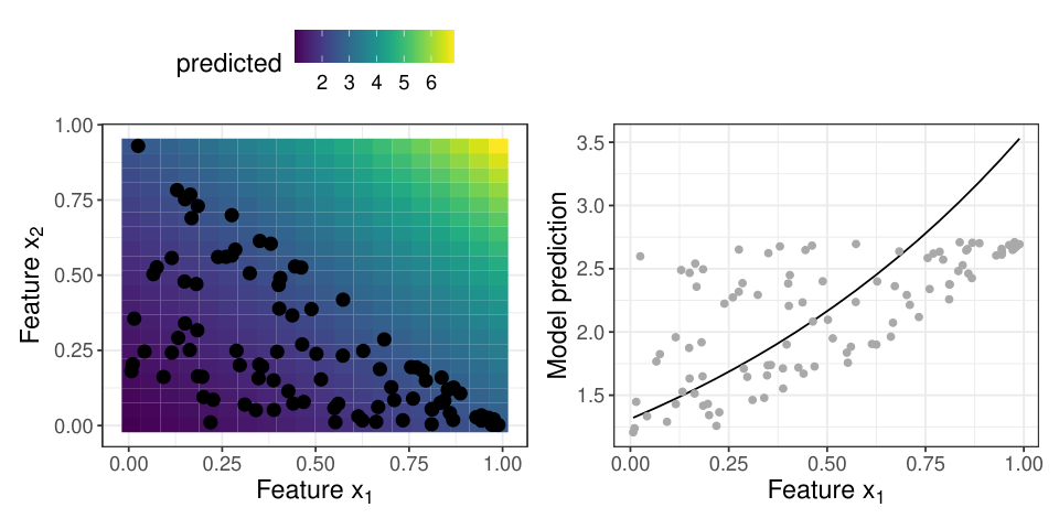
Extrapolation can be avoided by sampling a feature conditional on all other features and thereby preserving the joint distribution (Strobl et al. 2008; Hooker and Mentch 2019). This yields conditional variants of the PDP and PFI that have to be interpreted differently. While the interpretation of marginal PDP and PFI is independent of the other features, the interpretation of conditional PDP and PFI is conditional on other features.
Figure 2 shows how conditional PFI can be misinterpreted: Features and have the same coefficient in a linear model and the same marginal PFI, but has a lower conditional PFI since it is correlated with feature . The conditional PFI must be interpreted as the additional, unique contribution of a feature given all features we conditioned on (König et al. 2020; Fisher et al. 2019). It therefore has also been called “partial importance” (Debeer and Strobl 2020). If interpreted incorrectly, this can lead to the wrong conclusion that, for example, two strongly dependent features are irrelevant for the prediction model (Figure 2). The correct conclusion would be that a feature is less relevant given knowledge of the dependent feature.
In Figure 2, the conditional PDP shows a positive effect for a feature that has a negative coefficient in a linear regression model. The discrepancy is due to correlation of the feature with another feature with a large positive coefficient. The conditional effect of a feature is a mix of its marginal effect and the marginal effects of all dependent features (Hooker and Mentch 2019; Apley and Zhu 2016). While conditional PFI might assign a low importance to a feature on which the model relied heavily, the conditional PDP has the opposite pitfall: it can show an effect for a feature that was not used by the model. This interpretation might be undesirable and is similar to the omitted variable bias phenomenon, which also happens in Figure 2: regressing from , while ignoring (Apley and Zhu 2016).
The interpretation of conditional PFI and PDP requires knowledge of the dependence structure between the feature of interest and the other features. Such knowledge of dependence structures would help explain differences between a feature’s marginal and conditional PFI and break down the conditional PDP into the effect of the feature of interest and that of the dependent features. However, state-of-the-art conditional sampling mechanisms such as knockoffs (Barber et al. 2015; Candes et al. 2018; Watson and Wright 2019) do not provide a readily interpretable conditioning.
Our contributions are the following. We propose the conditional subgroup PDPs (cs-PDPs) and PFIs (cs-PFIs). Both are based on conditional subgroup permutation (cs-permutation), a sampling method for the conditional distribution. Standard (i.e., marginal) PDPs and PFIs are computed and interpreted within subgroups of the data, enabling a local interpretation of feature effect and importance while handling the problem of extrapolation. We construct the subgroups for a feature by training a decision tree in which the distribution of the feature becomes less dependent on other features. The tree structure allows interpretation of how other features influence the effect and importance of the feature at hand. We show that the conditional PFI estimate based on cs-PFIs can recover the ground truth in simulations and often outperforms related approaches. In addition, we study how well different conditional PDP/PFI approaches retain the joint distribution of data sets from the OpenML-CC18 benchmarking suite (Bischl et al. 2019) and show that cs-permutation achieves state-of-the-art data fidelity. We demonstrate that the cs-PDPs have a high model fidelity, that is, they are closer to the model prediction than other feature effect methods. By inspecting the cs-PFIs and cs-PDPs in combination with the respective subgroup descriptions, insights into the model and the dependence structure of the data are possible. We show how we can trade off human-intelligibility of the subgroups for extrapolation by choosing the granularity of the grouping. In an application, we illustrate how cs-PDPs and cs-PFIs can reveal new insights into the ML model and the data.
2 Notation and Background
We consider ML prediction functions , where is a model prediction and is a -dimensional feature vector. We use to refer to an observed feature (vector) and to refer to the -th feature as a random variable. With we refer to the complementary feature space and with to the corresponding random variables. We refer to the value of the -th feature from the -th instance as and to the tuples as data.
The Permutation Feature Importance (PFI) is defined as the increase in loss when feature is permuted:
| (1) |
If the random variable has the same marginal distribution as (e.g., permutation), the estimate yields the marginal PFI. If follows the conditional distribution , we speak of the conditional PFI. The PFI is estimated with the following formula:
| (2) |
where is the loss for the -th observation and is the loss where was replaced by the m-th sample . The latter refers to the -th feature value obtained by a sample of . The sample can be repeated -times for a more stable estimation of . Numerous variations of this formulation exist. Breiman 2001 proposed the PFI for random forests, which is computed from the out-of-bag samples of individual trees. Subsequently, Fisher et al. 2019 introduced a model-agnostic PFI version.
The marginal Partial Dependence Plot (PDP) (Friedman et al. 1991) describes the average effect of the j-th feature on the prediction.
| (3) |
If the expectation is conditional on , , we speak of the conditional PDP. The marginal PDP evaluated at feature value is estimated using Monte Carlo integration:
| (4) |
3 Related Work
In this section, we review conditional variants of PDP and PFI and other approaches that try to avoid extrapolation.
3.1 Related Work on Conditional PDP
The marginal plot (M-Plot) (Apley and Zhu 2016) averages the predictions locally on the feature grid and mixes effects of dependent features.
Hooker 2007 proposed a functional ANOVA decomposition with hierarchically orthogonal components, based on integration using the joint distribution of the data, which in practice is difficult to estimate.
Accumulated Local Effect (ALE) plots by Apley and Zhu 2016 reduce extrapolation by accumulating the finite differences computed within intervals of the feature of interest. By definition, interpretations of ALE plots are thus only valid locally within the intervals. Furthermore, there is no straightforward approach to derive ALE plots for categorical features, since ALE requires ordered feature values. Our proposed approach can handle categorical features.
Another PDP variant based on stratification was proposed by Parr and Wilson 2019. However, this stratified PDP describes only the data and is independent of the model.
Individual Conditional Expectation (ICE) curves by Goldstein et al. 2015 can be used to visualize the interactions underlying a PDP, but they also suffer from the extrapolation problem. The “conditional” in ICE refers to conditioning on individual observations and not on certain features. As a solution, Hooker and Mentch 2019 suggested to visually highlight the areas of the ICE curves in which the feature combinations are more likely.
3.2 Related Work on Conditional PFI
We review approaches that modify the PFI (Breiman 2001; Fisher et al. 2019) in presence of dependent features by using a conditional sampling strategy.
Strobl et al. 2008 proposed the conditional variable importance for random forests (CVIRF), which is a conditional PFI variant of Breiman 2001. CVIRF was further analyzed and extended by Debeer and Strobl 2020. Both CVIRF and our approach rely on permutations based on partitions of decision trees. However, there are fundamental differences. CVIRF is specifically developed for random forests and relies on the splits of the underlying individual trees of the random forest for the conditional sampling. In contrast, our cs-PFI approach trains decision trees for each feature using as features and as the target. Therefore, the subgroups for each feature are constructed from their conditional distributions (conditional on the other features) in a separate step, which is decoupled from the machine learning model to be interpreted. Our cs-PFI approach is model-agnostic, independent of the target to predict and not specific to random forests.
Hooker and Mentch 2019 made a general suggestion to replace feature values by estimates of .
Fisher et al. 2019 suggested to use matching and imputation techniques to generate samples from the conditional distribution. If has few unique combinations, they suggested to group by unique combinations and permute them for these fixed groups. For discrete and low-dimensional feature spaces, they suggest non-parametric matching and weighting methods to replace values. For continuous or high-dimensional data, they suggest imputing with and adding residuals (under the assumption of homogeneous residuals). Our approach using permutation in subgroups can be seen as a model-driven, binary weighting approach extended to continuous features.
Knockoffs (Candes et al. 2018) are random variables which are “copies” of the original features that preserve the joint distribution but are otherwise independent of the prediction target. Knockoffs can be used to replace feature values for conditional feature importance computation. Watson and Wright 2019 developed a testing framework for PFI based on knockoff samplers such as Model-X knockoffs (Candes et al. 2018). Our approach is complementary since Watson and Wright 2019 is agnostic to the sampling strategy that is used. Others have proposed to use generative adversarial networks for generating knockoffs (Romano et al. 2019). Knockoffs are not transparent with respect to how they condition on the features, while our approach creates interpretable subgroups.
Conditional importance approaches based on model retraining have been proposed (Hooker and Mentch 2019; Lei et al. 2018; Gregorutti et al. 2017). Retraining the model can be expensive, and answers a fundamentally different question, often related to feature selection and not based on a fixed set of features. Hence, we focus on approaches that compute conditional PFI for a fixed model without retraining.
None of the existing approaches makes the dependence structures between the features explicit. It is unclear which of the features in influenced the replacement of the most and how. Furthermore, little attention has been paid on evaluating how well different sampling strategies address the extrapolation problem. We address this gap with an extensive data fidelity experiment on the OpenML-CC18 benchmarking suite. To the best of our knowledge, our paper is also the first to conduct experiments using ground truth for the conditional PFI. Our approach works with any type of feature, be it categorical, numerical, ordinal and so on, since we rely on decision trees to find the subgroups used for conditioning. The differences between the different (conditional) PDP and PFI approaches ultimately boil down to how they sample from the conditional distribution. Table 1 lists different sampling strategies of model-agnostic interpretation methods and summarizes their assumptions to preserve the joint distribution.
| Sampling Strategy | Used/Suggested By | Assumptions |
|---|---|---|
| No intervention on | Drop-and-Refit, LOCO (Lei et al. 2018) | |
| Permute | Marginal PFI (Breiman 2001; Fisher et al. 2019), PDP (Friedman et al. 1991) | |
| Replace by knockoff with and | Knockoffs (Candes et al. 2018), CPI (Watson and Wright 2019) | |
| Move each to left and right interval bounds | ALE (Apley and Zhu 2016) | in intervals |
| Permute in subgroups | cs-PFI, cs-PDP | in subgroups |
| Permute in random forest tree nodes | CVIRF (Strobl et al. 2008; Debeer and Strobl 2020) | cond. on tree splits in to predict |
| Impute from | (Fisher et al. 2019) | Homogeneous residuals |
4 Conditional Subgroups
We suggest approaching the dependent feature problem by constructing an interpretable grouping such that the feature of interest becomes less dependent on remaining features within each subgroup. In the best case the features become independent: . Assuming that we find a grouping in which holds, sampling from the group-wise marginal distribution removes extrapolation (see Figure 3) and within each group, the samples from the marginal and the conditional distribution would coincide. Such groupings exist when, for example, the features in are categorical, or when the conditional distribution of only depends on discrete changes in features .
Such a grouping would consequently enable (1) the application of standard PFI and PDP within each group without extrapolation and (2) sampling from the global conditional distribution using group-wise permutation and aggregation.
With our approach we exploit these properties to derive both a group-wise marginal interpretation and, for the PFI, a global conditional interpretation.
Even when such a discrete grouping does not exist, e.g., when the true dependence is linear, the cs-permutation reduces extrapolation, see Figure 4.
Moreover, an accurate interpretation requires the groupings to be human-intelligible.
We can gain insight into how the model behaves within specific subgroups which is not possible with approaches that directly sample conditional on all features (Candes et al. 2018; Strobl et al. 2008; Aas et al. 2019; Fisher et al. 2019; Watson and Wright 2019).
For our approach, any algorithm can be used that splits the data in so that the distribution of becomes more homogeneous within a group and more heterogeneous between groups. We consider decision tree algorithms for this task, which predict based on splits in . Decision tree algorithms directly or indirectly optimize splits for heterogeneity of some aspects of the distribution of in the splits. The partitions in a decision tree can be described by decision rules that lead to that terminal leaf. We leverage this partitioning to construct an interpretable grouping based on random variable for a specific feature . The new variable can be calculated by assigning every observation the indicator of the partition that it lies in (meaning for observation with the group variable’s value is defined as ).
Transformation trees (trtr) (Hothorn and Zeileis 2017) are able to model the conditional distribution of a variable. This approach partitions the feature space so that the distribution of the target (here ) within the resulting subgroups is homogeneous, which means that the group-wise parameterization of the modeled distribution is independent of . Transformation trees directly model the target’s distribution , where is the chosen (cumulative) distribution function and a monotone increasing transformation function (hence the name transformation trees). The transformation function is defined as where is a basis function of polynomials or splines. The task of estimating the distribution is reduced to estimating , and the trees are split based on hypothesis tests for differences in given , and therefore differences in the distribution of . For more detailed explanations of transformation trees please refer to Hothorn and Zeileis 2017.
In contrast, a simpler approach would be to use classification and regression trees (CART) (Breiman et al. 1984), which, for regression, minimizes the variance within nodes, effectively finding partitions with different means in the distribution of . However, CART’s split criterion only considers differences in the expectation of the distribution of given : . This means CART could only make and independent if the distribution of only depends in its expectation on (and if the dependence can be modeled by partitioning the data). Any differences in higher moments of the distribution of such as the variance of cannot be detected.
We evaluated both trtr which are theoretically well equipped for splitting distributions and CART, which are established and well-studied. For the remainder of this paper, we have set the default minimum number of observations in a node to 30 for both approaches. For the transformation trees, we used the Normal distribution as target distribution and we used Bernstein polynomials of degree five for the transformation function. Higher-order polynomials do not seem to increase model fit further (Hothorn 2018).
We denote the subgroups by , where is the -th subgroup for feature , with groups in total for the -th feature. The subgroups per feature are disjoint: and . Let be a subset of that refers to the data subset belonging to the subgroup . Each subgroup can be described by the decision path that leads to the respective terminal node.
4.1 Remarks
4.1.1 Continuous Dependencies
For conditional independence to hold, the chosen decision tree approach has to capture the (potentially complex) dependencies between and . CART can only capture differences in the expected value of but are insensitive to changes in, for example, the variance. Transformation trees are in principle agnostic to the specified distribution and the default transformation family of distributions is very general, as empirical results suggest (Hothorn and Zeileis 2017). However, the approach is based on the assumption that the dependence can be modeled with a discrete grouping. For example, in the case of linear Gaussian dependencies, the corresponding optimal variable would be linear Gaussian itself, and would be in conflict with our proposed interpretable grouping approach. Even in these settings the approach allows an approximation of the conditional distribution. In the case of simple linear Gaussian dependencies, partitioning the feature space will still reduce extrapolation. But we never get rid of it completely, unless there are only individual data points left in each partition, see Figure 4.
4.1.2 Sparse Subgroups
Fewer subgroups are generally desirable for two reasons: (1) for a good approximation of the marginal distribution within a subgroup, a sufficient number of observations per group is required, which might lead to fewer subgroups, and (2) a large number of subgroups leads to more complex groups, which reduces their human-intelligibility and therefore forfeits the added value of the local, subgroup-wise interpretations. As we rely on decision trees, we can adjust the granularity of the grouping using hyperparameters such as the maximum tree depth. By controlling the maximum tree depth, we can control the trade-off between the depth of the tree (and hence its interpretability) and the homogeneity of the distribution within the subgroups.
4.2 Conditional Subgroup Permutation Feature Importance (cs-PFI)
We estimate the cs-PFI of feature within a subgroup as:
| (5) |
where refers to a feature value obtained from the -th permutation of within the subgroup . This estimation is exactly the same as the marginal PFI (Equation 2), except that it only includes observations from the given subgroup. Algorithm 1 describes the estimation of the cs-PFIs for a given feature on unseen data.
The algorithm has two outcomes: We get local importance values for feature for each subgroup (; Algorithm 1, line 8) and a global conditional feature importance (; Algorithm 1, line 9). The latter is equivalent to the weighted average of subgroup importances regarding the number of observations within each subgroup (see proof in Appendix A).
The cs-PFIs needs the same amount of model evaluations as the PFI (). On top of that comes the cost for training the respective decision trees and making predictions to assign a subgroup to each observation.
Theorem 4.1
When feature is independent of features for a given dataset , each has the same expectation as the marginal PFI, and an -times larger variance, where and are the number of observations in the data and the subgroup .
The proof of Theorem 4.1 is shown in Appendix B. Theorem 4.1 has the practical implication that even in the case of applying cs-PFI to an independent feature, we will retrieve the marginal PFI, and not introduce any problematic interpretations. Equivalence in expectation and higher variance under the independence of and holds true even if the partitions would be randomly chosen. Theorem 4.1 has further consequences regarding overfitting: Assuming a node has already reached independence between and , then further splitting the tree based on noise will not change the expected cs-PFIs.
4.3 Conditional Subgroup Partial Dependence Plots (cs-PDPs)
The conditional PDP has a different interpretation than the marginal PDP, as the motivating example in Figure 2 showed: The conditional PDP can be interpreted as the effect of a feature on the prediction, given that all other features would change according to the joint distribution. This violates a desirable property that the effect of features that were not used by the model should have a zero effect curve. This poses a dilemna for dependent features: Either extrapolate using the marginal PDP, or use the conditional PDP with undesirable properties for interpretation. Our proposed cs-PDPs reduces extrapolation while allowing a marginal interpretation within each subgroup. We compute the for each subgroup using the marginal PDP formula in Equation 4.
This results in multiple cs-PDPs per feature, which can be displayed together in the same plot as in Figure 12. As shown in Figure 5, even features that do not contribute to the prediction at all can have a conditional PDP different from zero. We therefore argue that an aggregation of the cs-PDPs to the conditional PDP is not meaningful for model interpretation, and we suggest to plot the group-wise curves. For the visualization of the cs-PDPs, we suggest to plot the PDPs similar to boxplots, where the dense center quartiles are indicated with a bold line (see Figure 6). We restrict each to the interval .
Equivalently to PFI, the subgroup PDPs approximate the true marginal PDP even if the features are independent.
Theorem 4.2
When feature is independent of features for a given dataset , each has the same expectation as the marginal PDP, and an -times larger variance, where and are the number of observations in the data and the subgroup .
The proof of Theorem 4.2 is shown in Appendix C. Theorem 4.2 has the same practical implications as Theorem 4.1: Even if the features are independent, we will, in expectation, get the marginal PDPs. And when trees are grown deeper than needed, in expectation the cs-PDPs will yield the same curve.
Both the PDP and the set of cs-PDPs need evaluations, since (and worst case if evaluated at each value). Again, there is an additional cost for training the respective decision trees and making predictions.
5 Training Conditional Sampling Approaches
To ensure that sampling approaches are not overfitting, we suggest to separate training and sampling, where training covers all estimation steps that involve data. For this purpose, we refer to the training data with and to the data for importance computation with . This section both describes how we compared the sampling approaches in the following chapters and serves as a general recommendation for how to use the sampling approaches.
For our cs-permutation, we trained the CART / transformation trees on and permuted of within the terminal nodes of the tree. For CVIRF (Strobl et al. 2008; Debeer and Strobl 2020), which is specific to random forests, we trained the random forest on to predict the target and permuted of within the terminal nodes. For Model-X knockoffs (Candes et al. 2018), we fitted the second-order knockoffs on and replaced in with its knockoffs. For the imputation approach (Fisher et al. 2019), we trained a random forest on to predict from , and replaced values of in with their random forest predictions plus a random residual. For the interval-based sampling (Apley and Zhu 2016), we computed quantiles of using and perturbed in by moving each observation once to the left and once to the right border of the respective intervals. The marginal permutation (PFI, PDP) required no training, we permuted (i.e., shuffled) the feature in .
6 Conditional PFI Ground Truth Simulation
We compared our cs-PFI approach using CART (tree cart) and transformation trees (tree trtr), CVIRF (Strobl et al. 2008; Debeer and Strobl 2020), Model-X knockoffs (ko) (Candes et al. 2018) and the imputation approach (impute rf) (Fisher et al. 2019) in ground truth simulations. We simulated the following data-generating process: , where . All features, except feature followed a Gaussian distribution: . Feature was simulated as a function of the other features plus noise: . We simulated the following scenarios by changing and :
- •
In the independent scenario, did not depend on any feature: , . This scenario served as a test how the different conditional PFI approaches handle the edge case of independence.
- •
The linear scenario introduces a strong correlation of with feature : , .
- •
In the non-linear scenario, we simulated as a non-linear function of multiple features: . Here also the variance of is a function of : .
- •
For the multiple linear dependencies scenario, we chose to depend on many features: , .
For each scenario, we varied the number of sampled data points and the number of features . To “train” each of the cPFI methods, we used (200 or 2000) data points and the rest (100 / 1000) to compute the cPFI. The experiment was repeated 1000 times. We examined two settings.
- •
In setting (I), we assumed that the model recovered the true model .
- •
In setting (II), we trained a random forest with 100 trees (Breiman 2001).
In both settings, the true conditional distribution of given the remaining features is known (function and error distribution is known). Therefore we can compute the ground truth conditional PFI, as defined in Equation 2. We generated the samples of according to to get the values and compute the increase in loss. The conditonal PFIs differed in settings (I) and (II) since in (I) we used the true , and in (II) the trained random forest .
6.1 Conditional PFI Ground Truth Results
For setting (I), the mean squared errors between the estimated conditional PFIs and the ground truth are displayed in Table 2, and the distributions of conditional PFI estimates in Figure 7. In the independent scenario, where conditional and marginal PFI are equal, all methods performed equally well, except in the low , high scenario, where the knockoffs sometimes failed. As expected, the variance was higher for all methods when . In the linear scenario, the marginal PFI was clearly different from the conditional PFI. There was no clear best performing conditional PFI approach, as the results differ depending on training size and number of features . For low and low , knockoffs performed best. For high , regardless of , the cs-permutation approaches worked best, which might be due to the feature selection mechanism inherent to trees. The multiple linear dependencies scenario was the only scenario in which the cs-PFI approach was consistently outperformed by the other methods. Decision trees already need multiple splits for recovering linear relationships, and in this scenario, multiple linear relationships had to be recovered. Imputation with random forest worked well when multiple linear dependencies are present. For knockoffs, the results were mixed. As expected, the cs-PFI approach worked well in the non-linear scenario, and outperformed all other approaches. Knockoffs and imputation with random forests both overestimated the conditional PFI (except for knockoffs for and ). In addition to this bias, they had a larger variance compared to the cs-PFI approaches.
Generally, the transformation trees performed equal to or outperformed CART across all scenarios, except for the multiple linear dependencies scenario. Our cs-PFI approaches worked well in all scenarios, except when multiple (linear) dependencies were present. Even for a single linear dependence, the cs-PFI approaches were on par with knockoffs and imputation, and clearly outperformed both when the relationship was more complex.
| setting | cs-PFI (cart) | cs-PFI (trtr) | impute rf | ko | mPFI |
|---|---|---|---|---|---|
| independent | |||||
| n=300, p=10 | 1.33 | 1.35 | 1.67 | 1.47 | 1.39 |
| n=300, p=90 | 1.50 | 1.29 | 1.46 | 5.81 | 1.31 |
| n=3000, p=10 | 0.14 | 0.15 | 0.16 | 0.13 | 0.15 |
| n=3000, p=90 | 0.15 | 0.14 | 0.14 | 0.18 | 0.13 |
| linear | |||||
| n=300, p=10 | 4.62 | 4.30 | 3.64 | 2.03 | 44.83 |
| n=300, p=90 | 5.55 | 5.26 | 17.53 | 11.63 | 45.36 |
| n=3000, p=10 | 0.40 | 0.26 | 0.26 | 0.63 | 37.40 |
| n=3000, p=90 | 0.45 | 0.31 | 3.55 | 0.38 | 36.32 |
| multi. lin. | |||||
| n=300, p=10 | 2443.67 | 2623.54 | 1276.41 | 1583.69 | 2739.83 |
| n=300, p=90 | 2574.54 | 2896.47 | 2141.01 | 6607.73 | 2988.68 |
| n=3000, p=10 | 1031.83 | 900.68 | 140.98 | 810.78 | 1548.37 |
| n=3000, p=90 | 1075.95 | 1041.10 | 438.25 | 185.13 | 1599.59 |
| non-linear | |||||
| n=300, p=10 | 22.00 | 17.76 | 265.73 | 668.34 | 1204.17 |
| n=300, p=90 | 19.99 | 19.81 | 504.53 | 131.77 | 1248.74 |
| n=3000, p=10 | 1.18 | 1.00 | 144.77 | 626.80 | 1156.32 |
| n=3000, p=90 | 1.17 | 1.13 | 206.01 | 579.02 | 1136.83 |
In setting (II), a random forest was analyzed, which allowed us to include the conditional variable importance for random forests (CVIRF) by Strobl et al. 2008; Debeer and Strobl 2020 in the benchmark. The MSEs are displayed in Appendix D, Table 7, and the distribution of conditional PFI estimates in Appendix D in Figure 14. The results for all other approaches are comparable to setting (I). For the low settings, CVIRF worked as well as the other approaches in the independent scenario. It outperformed the other approaches in the linear scenario and the multiple linear scenario (when was small). The CVIRF approach consistently underestimated the conditional PFI in all scenarios with high , even in the independent scenario. Therefore, we would recommend to analyze the conditional PFI for random forests using cs-PFI for lower dimensional dependence structures, and imputation for multiple (linear) dependencies.
7 Trading Interpretability for Accuracy
In an additional experiment, we examined the trade-off between the depth of the trees and the accuracy with which we recover the true conditional PFI. For scenario (I), we trained decision trees with different maximal depths (from 1 to 10) and analyzed how the resulting number of subgroups influenced the conditional PFI estimate. The experiment was repeated 1000 times. Figure 8 shows that the deeper the transformation trees (and the more subgroups), the better the true conditional PFI was approximated. The plot also shows that no overfitting occurred, which is in line with theoretical considerations in Theorem 4.1.
8 Data Fidelity Evaluation
PDP and PFI work by data intervention, prediction, and subsequent aggregation (Scholbeck et al. 2019). Based on data , the intervention creates a new data set. In order to compare different conditional sampling approaches, we define a measure of data fidelity to quantify the ability to preserve the joint distribution under intervention. Failing to preserve the joint distribution leads to extrapolation when features are dependent. Model-X knockoffs, for example, are directly motivated by preserving the joint distribution, while others, such as accumulated local effect plots do so more implicitly.
Data fidelity is the degree to which a sample of feature preserves the joint distribution, that is, the degree to which In theory, any measure that compares two multivariate distributions can be used to compute the data fidelity. In practice, however, the joint distribution is unknown, which makes measures such as the Kullback-Leibler divergence impractical. We are dealing with two samples, one data set without and one with intervention.
In this classic two-sample test-scenario, the maximum mean discrepancy (MMD) can be used to compare whether two samples come from the same distribution (Fortet and Mourier 1953; Smola et al. 2007; Gretton et al. 2007; Gretton et al. 2012). The empirical MMD is defined as:
| (6) |
where is the original data set and a data set with perturbed . For both data sets, we scaled numerical features to a mean of zero and a standard deviation of one. For the kernel we used the radial basis function kernel for all experiments. For parameter of the radial basis function kernel, we chose the median L2-distance between data points which is a common heuristic (Gretton et al. 2012). We measure data fidelity as the negative logarithm of the MMD () to obtain a more condensed scale where larger values are better.
Definition 1 (MMD-based Data Fidelity)
Let be a dataset, and be another dataset from the same distribution, but with an additional intervention. We define the data fidelity as: .
We evaluated how different sampling strategies (see Table 1) affect the data fidelity measure for numerous data sets of the OpenML-CC18 benchmarking suite (Bischl et al. 2019). We removed all data sets with 7 or fewer features and data sets with more than 500 features. See Appendix E for an overview of the remaining data sets. For each data set, we removed all categorical features from the analysis, as the underlying sampling strategies of ALE plots and Model-X knockoffs are not well equipped to handle them. We were foremost interested in two questions:
- A)
How does cs-permutation compare with other sampling strategies w.r.t. data fidelity?
- B)
How do choices of tree algorithm (CART vs. transformation trees) and tree depth parameter affect data fidelity?
In each experiment, we selected a data set, randomly sampled a feature and computed the data fidelity of various sampling strategies as described in the pseudo-code in Algorithm 2.
For an unbiased evaluation, we split the data into three pieces: (40% of rows), (30% of rows) and (30% of rows). We used to “train” each sampling method (e.g., train decision trees for cs-permutation, see Section 5). We used , which we left unchanged and , for which the chosen feature was perturbed to estimate the data fidelity. For each data set, we chose 10 features at random, for which sampling was applied. Marginal permutation (which ignores the joint distribution) and ”no perturbation” served as lower and upper bounds for data fidelity. For CVIRF, we only used one tree per random forest as we only compared the general perturbation strategy which is the same for each tree.
We repeated all experiments 30 times with different random seeds and therefore different data splits. All in all this produced results (42 data sets (up to) 10 features 30 repetitions) per sampling method. All results are shown in detail in Appendix E (Figures 15, 16, 17, 18).
Since the experiments are repeated across the same data sets and the same features, the data fidelity results are not independent. Therefore, we used a random intercept model (Bryk and Raudenbush 1992) to analyze the differences in data fidelity between different sampling approaches. The random intercepts were nested for each data set and each feature. We chose “Marginal Permutation” as the reference category. We fitted two random intercept models: One to compare cs-permutation with fully-grown trees (CART, trtr) with other sampling methods and another one to compare different tree depths.
8.1 Results A) State-of-the-art comparison
Figure 9 shows the effect estimates of different sampling approaches modeled with a random intercept model. The results show that cs-permutation performed better than all other methods. Model-X knockoffs and the imputation approach (with random forests) came in second place and outperformed ALE and CVIRF. Knockoffs were proposed to preserve the joint distribution, but are based on multivariate Gaussian distribution. This seems to be too restrictive for the data sets in our experiments. CVIRF does not have much higher data fidelity than marginal permutation. However, results for CVIRF must be viewed with caution, since data fidelity regards all features equally – regardless of their impact on the model prediction. For example, a feature can be highly correlated with the feature of interest, but might not be used in the random forest. A more informative experiment for comparing CVIRF can be found in Section 6. Figure 15 and Figure 16 in Appendix E show the individual data fidelity results for the OpenML-CC18 data sets. Not perturbing the feature at all has the highest data fidelity and serves as the upper bound. The marginal permutation serves as a lower baseline. For most data sets, cs-permutation has a higher data fidelity compared to all other sampling approaches. For all the other methods there is at least one data set on which they reach a low data fidelity (e.g., “semeion”, “qsar-biodeg” for ALE; “nodel-simulation”, “churn” for imputation; “jm1”, “pc1” for knockoffs). In contrast, cs-permutation achieves a consistently high data fidelity on all these data sets.
Additionally, we review the data fidelity rankings of the sampling methods in Table 3. The rankings show a similar picture as the random intercept model estimates, except that Model-X knockoffs have a better average ranking than imputation. This could be the case since on a few data sets (bank-marketing, electricity, see Figure 15 in Appendix E) Model-X knockoffs have a very low data fidelity but on most others a higher model fidelity than the imputation method.
| none | cs (trtr) | ko | cs (cart) | imp | ale | perm | cvirf | |
|---|---|---|---|---|---|---|---|---|
| Mean ranks | 2.50 | 3.51 | 3.70 | 3.76 | 4.25 | 4.61 | 6.82 | 6.84 |
| SD | 0.73 | 0.87 | 1.32 | 0.91 | 1.37 | 2.07 | 1.14 | 1.14 |
8.2 Results B) tree configuration
We included shallow trees with maximum depth parameter from 1 to 5 to analyze the trade-off between tree depth and data fidelity. We included trees with a maximum depth parameter of 30 (“fully-grown” trees as this was the software’s limit) as an upper bound for each decision tree algorithm. Figure 9 B) shows that the deeper the trees (and the more subgroups), the higher the data fidelity. This is to be expected, since deeper trees allow for a more fine-grained separation of distributions. More importantly, we are interested in the trade-off between depth and data fidelity. Even splitting with a maximum depth of only 1 (two subgroups) strongly improves data fidelity over the simple marginal permutation for most data sets. A maximum depth of two means another huge average improvement in data fidelity, and already puts cs-permutation on par with knockoffs. A depth of three to four is almost as good as a maximum depth parameter of 30 and already outperforms all other methods, while still being interpretable due to their shortness. CART slightly outperforms transformation trees clearly when trees are shallow, which is surprising since transformation trees are, in theory, better equipped to handle changes in the distribution. Deeply grown transformation trees (max. depth of 30) slightly outperform CART. Figure 17 and Figure 18 in Appendix E show data fidelity aggregated by data set.
9 Model Fidelity
Model fidelity has been defined as how well the predictions of an explanation method approximate the ML model (Ribeiro et al. 2016).
Similar to Szepannek 2019, we define model fidelity for feature effects as the mean squared error between model prediction and the prediction of the partial function (which depends only on feature ) defined by the feature effect method, for example .
For a given data instance with observed feature value , the predicted outcome of, for example, a PDP can be obtained by the value on the y-axis of the PDP at the observed value.
| (7) |
where is a feature effect function such as ALE or PDP. In order to evaluate ALE plots, they have to be adjusted such that they are on a comparable scale to a PDP (Apley and Zhu 2016): .
We trained random forests (500 trees), linear models and k-nearest neighbours models (k = 7) on various regression data sets (Table 4).
| wine | satellite | wind | space | pollen | quake | |
|---|---|---|---|---|---|---|
| No. of rows | 6497 | 6435 | 6574 | 3107 | 3848 | 2178 |
| No. of features | 12 | 37 | 15 | 7 | 6 | 4 |
70% of the data were used to train the ML models and the transformation trees / CARTs. This ensure that results are not over-confident due to overfitting, see also Section 5. The remaining 30% of the data were used to evaluate model fidelity. For each model and each data set, we measured model fidelity between effect prediction and model prediction (Equation 7), averaged across observations and features.
Table 5 shows that the model fidelity of ALE and PDP is similar, while the cs-PDPs have the best model fidelity. This is an interesting result since the decision trees for the cs-PDPs are neither based on the model nor on the real target, but solely on the conditional dependence structure of the features. However, the cs-PDPs have the advantage that we obtain multiple plots. We did not aggregate the plots to a single conditional PDP, but computed the model fidelity for the PDPs within the subgroups (visualized in Figure 12). Our cs-PDPs using trees with a maximum depth of 2 have a better model fidelity than using a maximum depth of 1. We limited the analysis to interpretable conditioning and therefore allowed only trees with a maximum depth of 2, since a tree depth of 3 already means up to 8 subgroups which is already an impractical number of PDPs to have in one plot. CART sometimes beats trtr (e.g., on the “satellite” data set) but sometimes trtr has a lower loss (e.g., on the “wind” data set). Using different models (knn or linear model) produced similar results, see Appendix F.
| pollen | quake | satellite | space | wind | wine | |
|---|---|---|---|---|---|---|
| PDP | 9.61 | 0.04 | 4.80 | 0.03 | 44.84 | 0.75 |
| ALE | 9.91 | 0.04 | 4.81 | 0.03 | 44.83 | 0.75 |
| cs-PDP trtr1 | 8.44 | 0.04 | 4.49 | 0.03 | 29.96 | 0.71 |
| cs-PDP cart1 | 8.44 | 0.04 | 3.71 | 0.03 | 31.38 | 0.73 |
| cs-PDP trtr2 | 8.17 | 0.04 | 3.25 | 0.03 | 26.56 | 0.70 |
| cs-PDP cart2 | 8.29 | 0.04 | 3.05 | 0.03 | 25.96 | 0.71 |
10 Application
In the following application, we demonstrate that cs-PDPs and cs-PFI are valuable tools to understand model and data beyond insights given by PFI, PDPs, or ALE plots. We trained a random forest to predict daily bike rentals (Dua and Graff 2017) with given weather and seasonal information. The data (, ) was divided into 70% training and 30% test data.
10.1 Analyzing Feature Dependence
The features in the bike data are dependent. For example, the correlation between temperature and humidity is 0.13. The data contains both categorical and numerical features and we are interested in the multivariate, non-linear dependencies. Thus, correlation is an inadequate measure of dependence. We therefore indicate the degree of dependence by showing the extent to which we can predict each feature from all other features in Table 6. This idea is based on the proportional reduction in loss (Cooil and Rust 1994). Per feature, we trained a random forest to predict that feature from all other features. We measured the proportion of loss explained to quantify the dependence of the respective feature on all other features. For numerical features, we used the R-squared measure. For categorical features, we computed , where is the mean misclassification error, the true class, the classification function of the random forest and the most frequent class in the training data. We divided the training data into two folds and trained the random forest on one half. Then, we computed the proportion of explained loss on the other half and vice versa. Finally, we averaged the results. The feature “work” can be fully predicted by weekday and holiday. Season, temperature, humidity and weather can be partially predicted and are therefore not independent.
| season | yr | holiday | weekday | temp | hum | work | weather | wind |
| 45% | 8% | 29% | 14% | 66% | 43% | 100% | 46% | 12% |
10.2 cs-PDPs and cs-PFI
To construct the subgroups, we used transformation trees with a maximum tree depth of 2 which limited the number of possible subgroups to 4.
Figure 10 shows that for most features the biggest change in the estimated conditional PFI happens when moving from a maximum depth of 0 (= marginal PFI) to a depth of 2. This makes a maximum depth of 2 a reasonable trade-off between limiting the number of subgroups and accurately approximating the conditional PFI. We compared the marginal and conditional PFI for the bike rental predictions, see Figure 11.
The most important features, according to (marginal) PFI, were temperature and year. For the year feature, the marginal and conditional PFI are the same. Temperature is less important when we condition on season and humidity. The season already holds a lot of information about the temperature, so this is not a surprise. When we know that a day is in summer, it is not as important to know the temperature to make a good prediction. On humid summer days, the PFI of temperature is zero. However, in all other cases, it is important to know the temperature to predict how many bikes will be rented on a given day. The disaggregated cs-PFI in a subgroup can be interpreted as “How important is the temperature, given we know that the season and the humidity”.
Both ALE and PDP show a monotone increase of predicted bike rentals up until a temperature of 25 ∘C and a decrease beyond that. The PDP shows a weaker negative effect of very high temperatures which might be caused by extrapolation: High temperature days are combined with e.g. winter. A limitation of the ALE plot is that we should only interpret it locally within each interval that was used to construct the ALE plot. In contrast, our cs-PDP is explicit about the subgroup conditions in which the interpretation of the cs-PDP is valid and shows the distributions in which the feature effect may be interpreted. The local cs-PDPs in subgroups reveal a more nuanced picture: For humid summer days, the temperature has no effect on the bike rentals, and the average number of rentals are below that of days with similar temperatures in spring, fall and drier summer days. The temperature has a slightly negative effect on the predicted number of bike rentals for dry summer days (humidity below 70.75).
The change in intercepts of the local cs-PDP can be interpreted as the effect of the grouping feature (season).
The slope can be interpreted as the temperature effect within a subgroup.
We also demonstrate the local cs-PDPs for the season, a categorical feature.
Figure 13 shows both the PDP and our local cs-PDPs.
The normal PDP shows that on average there is no difference between spring, summer and fall and only slightly less bike rentals in winter.
The PDP with four subgroups conditional on temperature shows that the marginal PDP is misleading.
The PDP indicates that in spring, summer and fall, around bikes are rented and in winter around fewer.
The cs-PDPs in contrast show that, conditional on temperature, the differences between the seasons are much greater, especially for low temperatures.
Only at high temperatures is the number of rented bikes similar between seasons.
11 Discussion
We proposed the cs-PFIs and cs-PDPs, wich are variants of PFI and PDP that work when features are dependent. Both cs-PFIs and cs-PDPs rely on permutations in subgroups based on decision trees. The approach is simple: Train a decision tree to predict the feature of interest and compute the (marginal) PFI / PDP in each terminal node defined by the decision tree.
Compared to other approaches, cs-PFIs and cs-PDPs enable a human comprehensible grouping, which carries information how dependencies affect feature effects and importance. As we showed in various experiments, our methods are on par or outperform other methods in many dependence settings. We therefore recommend using cs-PDPs and cs-PFIs to analyze feature effects and importances when features are dependent. However, due to their construction with decision trees, cs-PFIs and cs-PDPs do not perform well when the feature of interest depends on many other features, but only if it depends on a few features. We recommend analyzing the dependence structure beforehand, using the imputation approach with random forests in the case of multiple dependencies, and cs-PFIs in all other cases.
Our framework is flexible regarding the choice of partitioning and we leave the evaluation of the rich selection of possible decision tree and decision rules approaches to future research.
Reproducibility: All experiments were conducted using mlr (Lang et al. 2019) and R (R Core Team 2017). We used the iml package (Molnar et al. 2018) for ALE and PDP, party/partykit (Hothorn and Zeileis 2015) for CVIRF and knockoff (Patterson and Sesia 2020) for Model-X knockoffs. The code for all experiments is available at https://github.com/christophM/paper_conditional_subgroups.
Acknowledgements.
This project is funded by the Bavarian State Ministry of Science and the Arts, by the Bavarian Research Institute for Digital Transformation (bidt) and supported by the German Federal Ministry of Education and Research (BMBF) under Grant No. 01IS18036A and by the German Research Foundation (DFG), Emmy Noether Grant 437611051. The authors of this work take full responsibilities for its content.References
- Aas et al. (2019) Aas K, Jullum M, Løland A (2019) Explaining individual predictions when features are dependent: More accurate approximations to Shapley values. arXiv preprint arXiv:190310464
- Apley and Zhu (2016) Apley DW, Zhu J (2016) Visualizing the effects of predictor variables in black box supervised learning models. arXiv preprint arXiv:161208468
- Barber et al. (2015) Barber RF, Candès EJ, et al. (2015) Controlling the false discovery rate via knockoffs. The Annals of Statistics 43(5):2055–2085
- Bischl et al. (2019) Bischl B, Casalicchio G, Feurer M, Hutter F, Lang M, Mantovani RG, van Rijn JN, Vanschoren J (2019) Openml benchmarking suites. arXiv preprint arXiv:170803731
- Breiman (2001) Breiman L (2001) Random forests. Machine learning 45(1):5–32
- Breiman et al. (1984) Breiman L, Friedman J, Olshen R, Stone C (1984) Classification and Regression Trees. Wadsworth and Brooks
- Bryk and Raudenbush (1992) Bryk AS, Raudenbush SW (1992) Hierarchical linear models: Applications and data analysis methods. Sage Publications, Inc
- Candes et al. (2018) Candes E, Fan Y, Janson L, Lv J (2018) Panning for gold:‘model-x’knockoffs for high dimensional controlled variable selection. Journal of the Royal Statistical Society: Series B (Statistical Methodology) 80(3):551–577
- Casalicchio et al. (2017) Casalicchio G, Bossek J, Lang M, Kirchhoff D, Kerschke P, Hofner B, Seibold H, Vanschoren J, Bischl B (2017) OpenML: An R package to connect to the machine learning platform OpenML. Comput Stat
- Cooil and Rust (1994) Cooil B, Rust RT (1994) Reliability and expected loss: A unifying principle. Psychometrika 59(2):203–216
- Debeer and Strobl (2020) Debeer D, Strobl C (2020) Conditional permutation importance revisited. BMC bioinformatics 21(1):1–30
- Dua and Graff (2017) Dua D, Graff C (2017) UCI machine learning repository. URL http://archive.ics.uci.edu/ml
- Fisher et al. (2019) Fisher A, Rudin C, Dominici F (2019) All models are wrong, but many are useful: Learning a variable’s importance by studying an entire class of prediction models simultaneously. Journal of Machine Learning Research 20(177):1–81
- Fortet and Mourier (1953) Fortet R, Mourier E (1953) Convergence de la répartition empirique vers la répartition théorique. In: Annales scientifiques de l’École Normale Supérieure, vol 70, pp 267–285
- Friedman et al. (1991) Friedman JH, et al. (1991) Multivariate adaptive regression splines. The annals of statistics 19(1):1–67
- Goldstein et al. (2015) Goldstein A, Kapelner A, Bleich J, Pitkin E (2015) Peeking inside the black box: Visualizing statistical learning with plots of individual conditional expectation. J Comput Graph Stat 24(1):44–65
- Gregorutti et al. (2017) Gregorutti B, Michel B, Saint-Pierre P (2017) Correlation and variable importance in random forests. Statistics and Computing 27(3):659–678
- Gretton et al. (2007) Gretton A, Fukumizu K, Teo CH, Song L, Schölkopf B, Smola AJ, et al. (2007) A kernel statistical test of independence. In: Nips, Citeseer, vol 20, pp 585–592
- Gretton et al. (2012) Gretton A, Borgwardt KM, Rasch MJ, Schölkopf B, Smola A (2012) A kernel two-sample test. The Journal of Machine Learning Research 13(1):723–773
- Guidotti et al. (2018) Guidotti R, Monreale A, Ruggieri S, Turini F, Giannotti F, Pedreschi D (2018) A survey of methods for explaining black box models. ACM computing surveys (CSUR) 51(5):1–42
- Hooker (2007) Hooker G (2007) Generalized functional anova diagnostics for high-dimensional functions of dependent variables. J Comput Graph Stat 16(3)
- Hooker and Mentch (2019) Hooker G, Mentch L (2019) Please stop permuting features: An explanation and alternatives. arXiv preprint arXiv:190503151
- Hothorn (2018) Hothorn T (2018) Top-down transformation choice. Statistical Modelling 18(3-4):274–298
- Hothorn and Zeileis (2015) Hothorn T, Zeileis A (2015) partykit: A modular toolkit for recursive partytioning in r. The Journal of Machine Learning Research 16(1):3905–3909
- Hothorn and Zeileis (2017) Hothorn T, Zeileis A (2017) Transformation forests. arXiv preprint arXiv:170102110
- König et al. (2020) König G, Molnar C, Bischl B, Grosse-Wentrup M (2020) Relative feature importance. arXiv preprint arXiv:200708283
- Lang et al. (2019) Lang M, Binder M, Richter J, Schratz P, Pfisterer F, Coors S, Au Q, Casalicchio G, Kotthoff L, Bischl B (2019) mlr3: A modern object-oriented machine learning framework in R. Journal of Open Source Software
- Lei et al. (2018) Lei J, G’Sell M, Rinaldo A, Tibshirani RJ, Wasserman L (2018) Distribution-free predictive inference for regression. Journal of the American Statistical Association 113(523):1094–1111
- Molnar (2019) Molnar C (2019) Interpretable Machine Learning. https://christophm.github.io/interpretable-ml-book/
- Molnar et al. (2018) Molnar C, Bischl B, Casalicchio G (2018) iml: An R package for interpretable machine learning. JOSS 3(26):786
- Molnar et al. (2020) Molnar C, König G, Herbinger J, Freiesleben T, Dandl S, Scholbeck CA, Casalicchio G, Grosse-Wentrup M, Bischl B (2020) Pitfalls to avoid when interpreting machine learning models. arXiv preprint arXiv:200704131
- Parr and Wilson (2019) Parr T, Wilson JD (2019) A stratification approach to partial dependence for codependent variables. arXiv preprint arXiv:190706698
- Patterson and Sesia (2020) Patterson E, Sesia M (2020) knockoff: The Knockoff Filter for Controlled Variable Selection. URL https://CRAN.R-project.org/package=knockoff, r package version 0.3.3
- R Core Team (2017) R Core Team (2017) R: A Language and Environment for Statistical Computing. R Foundation for Statistical Computing, Vienna, Austria
- Ribeiro et al. (2016) Ribeiro MT, Singh S, Guestrin C (2016) Why should i trust you?: Explaining the predictions of any classifier. In: Proceedings of the 22nd ACM SIGKDD international conference on knowledge discovery and data mining, ACM, pp 1135–1144
- Romano et al. (2019) Romano Y, Sesia M, Candès E (2019) Deep knockoffs. Journal of the American Statistical Association pp 1–12
- Scholbeck et al. (2019) Scholbeck CA, Molnar C, Heumann C, Bischl B, Casalicchio G (2019) Sampling, intervention, prediction, aggregation: A generalized framework for model-agnostic interpretations. In: Joint European Conference on Machine Learning and Knowledge Discovery in Databases, Springer, pp 205–216
- Smola et al. (2007) Smola A, Gretton A, Song L, Schölkopf B (2007) A hilbert space embedding for distributions. In: International Conference on Algorithmic Learning Theory, Springer, pp 13–31
- Strobl et al. (2008) Strobl C, Boulesteix AL, Kneib T, Augustin T, Zeileis A (2008) Conditional variable importance for random forests. BMC bioinformatics 9(1):307
- Szepannek (2019) Szepannek G (2019) How much can we see? A note on quantifying explainability of machine learning models. arXiv preprint arXiv:191013376
- Toloşi and Lengauer (2011) Toloşi L, Lengauer T (2011) Classification with correlated features: unreliability of feature ranking and solutions. Bioinformatics 27(14):1986–1994
- Vanschoren et al. (2014) Vanschoren J, Van Rijn JN, Bischl B, Torgo L (2014) OpenML: networked science in machine learning. ACM SIGKDD Explorations Newsletter 15(2):49–60
- Watson and Wright (2019) Watson DS, Wright MN (2019) Testing conditional independence in supervised learning algorithms. arXiv preprint arXiv:190109917
Appendix A Decompose conditional PFI into cs-PFIs
Assuming a perfect construction of , it holds that and also that (as is a compression of ). Therefore
| (8) |
When we sample the replacement for an from the marginal within a group (, e.g., via permutation) we also sample from the conditional . Every data point from the global sample can therefore equivalently be seen as a sample from the marginal within the group, or as a sample from the global conditional distribution.
As follows, the weighted sum of marginal subgroup PFIs coincides with the conditional PFI (cPFI).
| (9) | ||||
| (10) | ||||
| (12) |
Appendix B Expectation and Variance of the PFI in a Subgroup
We show that under feature independence the PFI and a PFI in an arbitrary subgroup have the same expected value and the subgroup PFI has a higher variance. Let and .
Proof
Appendix C Expectation and Variance of the PDP in a Subgroup
We show that under feature independence the PDP and a PDP in an arbitrary subgroup have the same expected value and the subgroup PDP has a higher variance.
Proof
Appendix D cPFI Ground Truth Scenario II
This chapter contains the results for the conditional PFI ground truth simulation, scenario II with an intermediate random forest.
| setting | cs-PFI (cart) | cs-PFI (trtr) | cvirf | impute rf | ko | mPFI |
|---|---|---|---|---|---|---|
| independent | ||||||
| n=300, p=10 | 0.26 | 0.28 | 0.22 | 0.27 | 0.25 | 0.27 |
| n=300, p=90 | 0.19 | 0.17 | 0.14 | 0.18 | 0.19 | 0.17 |
| n=3000, p=10 | 0.07 | 0.07 | 1.39 | 0.07 | 0.06 | 0.08 |
| n=3000, p=90 | 0.08 | 0.08 | 1.37 | 0.08 | 0.08 | 0.08 |
| linear | ||||||
| n=300, p=10 | 1.79 | 1.69 | 0.45 | 1.87 | 1.10 | 7.11 |
| n=300, p=90 | 1.93 | 1.88 | 1.36 | 4.25 | 2.93 | 7.06 |
| n=3000, p=10 | 0.29 | 0.22 | 5.41 | 0.25 | 0.40 | 6.80 |
| n=3000, p=90 | 0.32 | 0.24 | 6.98 | 1.66 | 0.26 | 7.02 |
| multi. lin. | ||||||
| n=300, p=10 | 667.79 | 744.48 | 275.58 | 335.40 | 377.35 | 726.15 |
| n=300, p=90 | 972.42 | 1098.74 | 301.26 | 823.89 | 1473.67 | 1065.26 |
| n=3000, p=10 | 715.41 | 625.99 | 1790.45 | 114.71 | 454.26 | 1017.53 |
| n=3000, p=90 | 974.37 | 945.19 | 5090.09 | 532.44 | 110.94 | 1416.30 |
| non-linear | ||||||
| n=300, p=10 | 1.40 | 1.29 | 1.37 | 3.96 | 12.35 | 18.51 |
| n=300, p=90 | 1.06 | 1.03 | 2.05 | 6.77 | 2.38 | 12.32 |
| n=3000, p=10 | 0.17 | 0.16 | 6.53 | 1.55 | 15.29 | 17.56 |
| n=3000, p=90 | 0.15 | 0.14 | 9.09 | 3.28 | 8.00 | 11.30 |
Appendix E Data Fidelity on OpenML-CC18 data sets
An overview of data sets from the OpenML-CC18 benchmarking suit. We used a subset of 42 out of 72 data sets with 7 to 500 continuous features.
| OpenML ID | Name | No. Obs. | No. numerical feat. | No. feat. |
|---|---|---|---|---|
| 1049 | pc4 | 1458 | 38 | 38 |
| 1050 | pc3 | 1563 | 38 | 38 |
| 1053 | jm1 | 10880 | 22 | 22 |
| 1063 | kc2 | 522 | 22 | 22 |
| 1067 | kc1 | 2109 | 22 | 22 |
| 1068 | pc1 | 1109 | 22 | 22 |
| 12 | mfeat-factors | 2000 | 217 | 217 |
| 14 | mfeat-fourier | 2000 | 77 | 77 |
| 1461 | bank-marketing | 45211 | 8 | 17 |
| 1475 | first-order-theorem-proving | 6118 | 52 | 52 |
| 1480 | ilpd | 583 | 10 | 11 |
| 1486 | nomao | 34465 | 90 | 119 |
| 1487 | ozone-level-8hr | 2534 | 73 | 73 |
| 1494 | qsar-biodeg | 1055 | 42 | 42 |
| 1497 | wall-robot-navigation | 5456 | 25 | 25 |
| 15 | breast-w | 683 | 10 | 10 |
| 1501 | semeion | 1593 | 257 | 257 |
| 151 | electricity | 45312 | 8 | 9 |
| 1510 | wdbc | 569 | 31 | 31 |
| 16 | mfeat-karhunen | 2000 | 65 | 65 |
| 182 | satimage | 6430 | 37 | 37 |
| 188 | eucalyptus | 641 | 15 | 20 |
| 22 | mfeat-zernike | 2000 | 48 | 48 |
| 23517 | numerai28.6 | 96320 | 22 | 22 |
| 28 | optdigits | 5620 | 63 | 65 |
| 307 | vowel | 990 | 11 | 13 |
| 31 | credit-g | 1000 | 8 | 21 |
| 32 | pendigits | 10992 | 17 | 17 |
| 37 | diabetes | 768 | 9 | 9 |
| 40499 | texture | 5500 | 41 | 41 |
| 40701 | churn | 5000 | 17 | 21 |
| 40966 | MiceProtein | 552 | 78 | 82 |
| 40979 | mfeat-pixel | 2000 | 241 | 241 |
| 40982 | steel-plates-fault | 1941 | 28 | 28 |
| 40984 | segment | 2310 | 19 | 20 |
| 40994 | climate-model-simulation-crashes | 540 | 21 | 21 |
| 44 | spambase | 4601 | 58 | 58 |
| 4538 | GesturePhaseSegmentationProcessed | 9873 | 33 | 33 |
| 458 | analcatdata_authorship | 841 | 71 | 71 |
| 54 | vehicle | 846 | 19 | 19 |
| 6 | letter | 20000 | 17 | 17 |
| 6332 | cylinder-bands | 378 | 19 | 40 |