Bayesian beta nonlinear models with constrained parameters to describe ruminal degradation kineticsThe original article is published in Journal of Applied Statistics. Published online: 09 Apr 2021, https://doi.org/10.1080/02664763.2021.1913105. This reprint differs from the original in pagination and typographic detail.
Abstract
The models used to describe the kinetics of ruminal degradation are usually nonlinear models where the dependent variable is the proportion of degraded food. The method of least squares is the standard approach used to estimate the unknown parameters but this method can lead to unacceptable predictions. To solve this issue, a beta nonlinear model and the Bayesian perspective is proposed in this article. The application of standard methodologies to obtain prior distributions, such as the Jeffreys prior or the reference priors, involves serious difficulties here because this model is a nonlinear non-normal regression model, and the constrained parameters appear in the log-likelihood function through the Gamma function. This paper proposes an objective method to obtain the prior distribution, which can be applied to other models with similar complexity, can be easily implemented in OpenBUGS, and solves the problem of unacceptable predictions. The model is generalized to a larger class of models. The methodology was applied to real data with three models that were compared using the Deviance Information Criterion and the root mean square prediction error. A simulation study was performed to evaluate the coverage of the credible intervals.
Keywords: Bayesian analysis; Beta regression; Default prior distributions; MCMC; Ruminal degradation kinetics
1 Introduction
Feed ingested by ruminant animals is subjected to degradation in the rumen, and the final products of the degradation are used for the synthesis of microbial biomass. The nutritional value of a feed depends on its nutrient content, the extent of degradation and the digestibility of non-degraded food components. To evaluate the nutritional status of ruminant animals and to predict the amount of nutrients required, the accurate estimation of the degradation of the feed that they receive is paramount.
The model proposed by Ørskov and McDonald Ørskov and McDonald 1979 is widely used to describe the kinetics of ruminal degradation and to provide information on the quality and nutritional characteristics of food. According to the main collection of the Web of Science, this model has been cited by at least 3029 research articles. The model assumes that , the proportion of degraded food up to time , is given by the nonlinearizable curve , where means the proportion of degraded food almost instantaneously and means the remaining proportion of food to be degraded at a velocity that is controlled by . Due to the biological meaning of these parameters, they have to satisfy the following constraints: , , , and .
The method of least squares is the standard approach used to estimate the unknown parameters , , and . This method presents two deficiencies for this problem. First, the distributions of the estimators are unknown, and hence, asymptotic approximations are usually used in standard statistical packages to obtain standard errors and confidence intervals. However, very often, the sample size is not large enough in the experiments performed to study degradation kinetic curves, which limits the application of asymptotic approximations. Second, and perhaps more important, the method can lead to unacceptable predictions if the estimates do not satisfy the above constraints on , , and . For instance, the data , , have been obtained from Ørskov and McDonald 1979, the unrestricted maximum likelihood estimates of , , and are , , and , respectively, and the frequentist 95% confidence intervals are (-0.0178, 0.4380), (0.5336, 1.1210), and (-0.0164, 0.1648), respectively. The confidence intervals contain inadmissible values, , and for , the prediction of the proportion of food degraded is .
Cano and Salmerón Cano and Salmerón 2007 have shown that the Bayesian approach avoids these disadvantages automatically if the constraints are taken into account in the prior distribution and consequently in the posterior distribution. On the other hand, the Bayesian model in Cano and Salmerón 2007 assumes that the distribution of the observed proportions is the normal distribution; concretely, if is the observed proportion at times , , then the model assumes that
| (1) |
However, the data are proportions, and hence, the normal distribution might not be suitable. A reasonable solution to improve the model could be to apply a transformation, such as the logit or the log-log, and then to assume that the distribution of the transformed data is normal. However, this procedure does not allow imposing that the mean of is in a treatable way. Suppose that the transformation is and that the model for is . To obtain
we would need to solve as a function of , which complicates the inference procedure. The solution adopted in this article models the proportion using the beta distribution.
The proposed model is a beta nonlinear regression model, and it is presented in section 2. The model takes advantage of the parameterization used in Ferrari and Cribari-Neto 2004, but the mean of the response variable, , is expressed as to preserve the interpretation of the parameters instead of using the logit link function as in Ferrari and Cribari-Neto 2004. In section 3, a prior distribution is proposed that takes into account the interpretation of the parameters, and how the Bayesian model can be implemented in OpenBugs is demonstrated. Although the model of Ørskov and McDonald is widely used, these results are generalized to a large class of models in section 4. Section 5 is dedicated to illustrating the procedure with real and simulated data.
2 The beta nonlinear regression model
Let be the independent observed proportions of degraded food at times , where . The beta distribution with density function
where , is used to model these proportions. To adapt the deterministic equation proposed by Ørskov and McDonald Ørskov and McDonald 1979, the expected value of is modelled as . Concretely, the proposed model is such that
| (2) |
, where , , , , and . The restrictions on the parameters ensure that model (2) is well defined because .
The mean and variance of are given by
and
respectively, and therefore, can be interpreted as a precision parameter.
Model (2) is a nonlinear regression model with beta response and constraints on the unknown parameters, and the log-likelihood function of for the sample is
| (3) |
where , , , , . Hence, neither the frequentist nor the Bayesian approach is implemented by default in the standard statistical packages. The Bayesian approach is considered in this article.
3 The prior distribution
When prior information is not available, default prior distributions such as the Jeffreys prior, see Jeffreys 1961, or the reference priors, see Bernardo 1979, Berger and Bernardo 1989, and Berger and Bernardo 1992, are usually recommended. However, these prior distributions are difficult to obtain for models such as (2) because this model is a nonlinear non-normal regression model, and the parameters appear in the log-likelihood function (3) through the Gamma function. Note that in model (2) cannot be expressed in the framework of the generalized linear models; that is, there is no link function such that is a linear combination of the unknown parameters , , and , as in Ferrari and Cribari-Neto 2004. The procedure used here is different and allows us to easily implement the resulting model using OpenBUGS. The argument for developing a prior distribution is as follows.
The prior distribution considered is of the form
Because and are proportions and is also a proportion, the uniform distribution
is a sensible prior distribution.
Now, consider that , , and are known, and we wish to obtain a prior distribution for . Let be an arbitrary observation time. Because of and , then . Since the unknown parameter is the expected proportion at time , the uniform prior for is a reasonable choice, and then the prior distribution of should be
| (4) |
Because the choice of is arbitrary, the proposal is the average
Finally, a diffuse gamma prior is proposed for because this parameter can be interpreted as a precision parameter.
The resulting prior distribution is not a standard prior, but it can be implemented using OpenBugs because is a mixture of exponential distributions, , and
is the density of the beta . On the other hand, as one of the reviewers of the article has suggested, we can interpret in terms of a Dirichlet distribution on a 2-simplex and the relationship with the gamma distribution, that is, we can consider:
where the distribution of , , and , is the exponential distribution .
The model in BUGS language is as follows:
Ψmodel
Ψ{
ΨΨfor(i in 1 : n) {
ΨΨΨy[i] ~ dbeta(p[i],q[i])
ΨΨΨp[i]<-mu[i]*tau
ΨΨΨq[i]<-tau-p[i]
ΨΨΨmu[i] <-min(a+b*(1-exp(-c*t[i])),1)
ΨΨΨ#Take min to prevent numerical problems
ΨΨΨP[i]<-1/n
ΨΨ}
ΨΨa.star ~ dexp(1)
ΨΨb.star ~ dexp(1)
ΨΨd ~ dexp(1)
ΨΨ
ΨΨa<-a.star/suma
ΨΨb<-b.star/suma
ΨΨsuma<-a.star+b.star+d
ΨΨ
ΨΨc ~ dexp(t[j])
ΨΨj ~ dcat(P[])
ΨΨtau ~ dgamma(0.001,0.001)
Ψ}
Note that if one solves the equation and assumes the uniform distribution for , then
which is equivalent to the exponential distribution (4).
This model have been implemented using Stan, see supplementary material.
4 Generalization to other models
The model proposed by Ørskov and McDonald Ørskov and McDonald 1979 is the most commonly used model to describe ruminal degradation kinetics. However, other models have been used to describe forage degradation kinetics during incubation in the rumen; see France et al. 1993, France et al. 2000, Dhanoa et al. 1995, Dhanoa et al. 2000, Dhanoa et al. 2004, López et al. 1999, Thornley and France 2006, and Nasri et al. 2006. Most of these models can be written as , where the meanings of and are the same as that in the model proposed by Ørskov and McDonald 1979, is an unknown parameter, and the function is a positive monotonically increasing function with , that is, the distribution function of a positive random variable . For example, for the model , the function is the exponential distribution, and for the Michaelis-Mentel model, is the distribution of a random variable whose logarithm has a logistic distribution. Other examples for appear in the appendix; some of them have been previously applied to explain ruminal degradation using the least squares to estimate the unknown parameters.
Considering a general distribution function allows generalizing model (2) as follows:
| (5) |
, where , , , , , and is a distribution function on for each .
The arguments for choosing the prior distribution are similar to the previous ones for model (2). Again, . Let be the dimension of . Then, given , since
| (6) |
if the uniform distribution is assumed for , , in the set defined by (6) with , then the prior distribution of should be proportional to
under some regularity conditions on the function . Note that for model (2), it follows that , , and the set defined by (6) is the interval .
Alternatively, one can solve the system of equations
| (7) |
obtaining as a function of , where the distribution of is the uniform distribution in the set defined by (7) with .
Since the choice is arbitrary, the proposal for is the average among all the subsets with . Again, a diffuse gamma prior is proposed for .
4.1 The Michaelis-Mentel model
This model is described by the equation , with , and . Then,
and therefore
The density is the density of the random variable , where . This is equivalent to solving the equation . Hence, this prior can be implemented in OpenBUGS as follows:
Ψmodel
Ψ{
ΨΨfor(i in 1 : n) {
ΨΨΨy[i] ~ dbeta(p[i],q[i])
ΨΨΨp[i]<-mu[i]*tau
ΨΨΨq[i]<-tau-p[i]
ΨΨΨmu[i]<-min(a+b*t[i]/(xi+t[i]),1)
ΨΨΨ#Take min to prevent numerical problems
ΨΨΨP[i]<-1/n
ΨΨ}
ΨΨa.star ~ dexp(1)
ΨΨb.star ~ dexp(1)
ΨΨd ~ dexp(1)
ΨΨ
ΨΨa<-a.star/suma
ΨΨb<-b.star/suma
ΨΨsuma<-a.star+b.star+d
ΨΨ
ΨΨu ~ dunif(0,1)
ΨΨxi <- t[j]*(1-u)/u
ΨΨj ~ dcat(P[])
ΨΨtau ~ dgamma(0.001,0.001)
Ψ}
4.2 The France model
France et al. France et al. 1993 have proposed the model , with
where , and . This model generalizes the model proposed by Ørskov and McDonald Ørskov and McDonald 1979.
In this case, system of equations (7) is
and the solution is
Therefore, the model in BUGS language is as follows:
Ψmodel
Ψ{
ΨΨfor(i in 1 : n) {
ΨΨΨy[i] ~ dbeta(p[i],q[i])
ΨΨΨp[i]<-mu[i]*tau
ΨΨΨq[i]<-tau-p[i]
ΨΨΨmu[i]<-min(a+b*(1-exp(-abs(xi1)*t[i]-abs(xi2)*sqrtt[i])),1)
ΨΨΨ#Take min and absolute values to prevent numerical problems
ΨΨΨP[i]<-1/n
ΨΨΨsqrtt[i] <- sqrt(t[i])
ΨΨ}
ΨΨa.star ~ dexp(1)
ΨΨb.star ~ dexp(1)
ΨΨd ~ dexp(1)
ΨΨ
ΨΨa<-a.star/suma
ΨΨb<-b.star/suma
ΨΨsuma<-a.star+b.star+d
ΨΨ
ΨΨxi1 <- (-sqrtt[j1]*lu1+sqrtt[j2]*lu2)/deno
ΨΨxi2 <- (-t[j2]*lu2+t[j1]*lu1)/deno
ΨΨdeno <- t[j2]*sqrtt[j1]-t[j1]*sqrtt[j2]
ΨΨlu1 <- log(1-u1)
ΨΨlu2 <- log(1-u2)
ΨΨj1 ~ dcat(P[])
ΨΨj2 ~ dcat(P[])
ΨΨu1 ~ dunif(0,1)
ΨΨu2 ~ dunif(0,1)
ΨΨtau ~ dgamma(0.001,0.001)
ΨΨ
ΨΨzero1<-0
ΨΨzero1~dbern(C1)
ΨΨC1 <- step(-xi1)
ΨΨ
ΨΨzero2<-0
ΨΨzero2~dbern(C2)
ΨΨC2 <- step(-xi2)
ΨΨ
ΨΨzero3<-0
ΨΨzero3~dbern(C3)
ΨΨC3<-equals(deno,0)
Ψ}
Note that the conditions and have been imposed.
Unfortunately, is not always related to a standard prior as in model (2). For example, for the Gompertz model,
the Jacobian determinant is
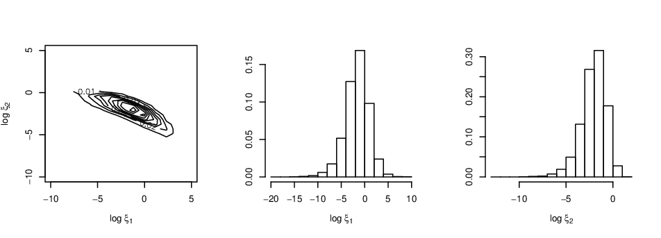
and system of equations (7) has no analytical solution in general. However, we can use a standard prior and then apply sampling importance resampling (see Smith and Gelfand 1992): after running OpenBUGS, the simulations are weighted with weights proportional to . In this case, the prior distribution can be obtained using simulation and kernel density estimation with statistical packages as np; see Hayfield and Racine 2008. The simulation from can be performed simulating the set , , , and solving (7) in the set . For example, for the Gompertz model 30000 simulations of have been performed with this procedure and the contour plot and histograms are represented in Figure 1 when .
5 Examples
5.1 Orskov and McDonald’s experiment
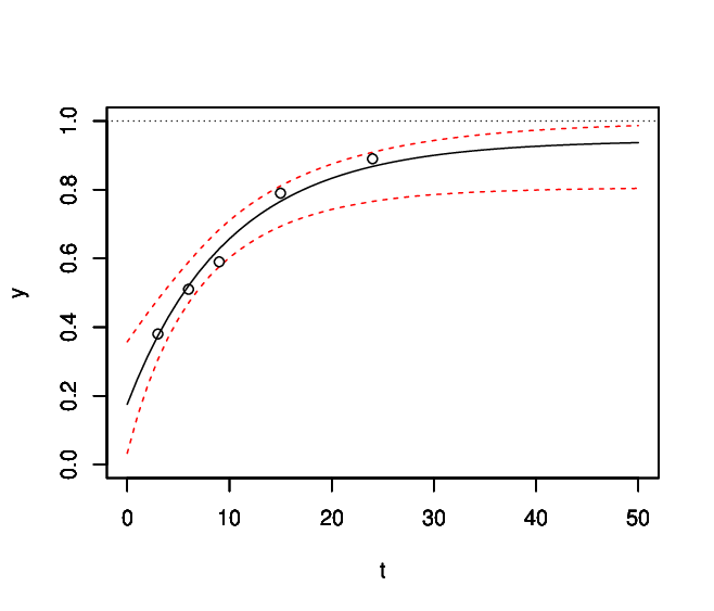
The model (2) implemented in OpenBugs was used with 3 chains, each with 50000 iterations (the first 1000 were discarded). The Bayesian estimates are shown in Table 1, and the posterior estimation of the curve for is shown in Figure 2. We can observe that the prediction for the degraded food is always between 0 and 1, as well as the 95%CI, unlike what happens with the least squares method. Table 1 shows that credible intervals do not contain immissable values. In fact, the posterior mean of was 0.946, and the 95%CI was (0.816, 0.998). The potential scale reduction factors ranged from 1.001 to 1.005, and Figures 3 and 4 show trace, autocorrelation and density for the parameters, indicating that the convergence was achieved.
In addition, the Michaelis-Mentel model and the France model were implemented in OpenBugs with 3 chains, each with 50000 iterations (first 1000 discarded). The potential scale reduction factors ranged from 1.001 to 1.015. The posterior mean of the potential degradability () was very similar for the three the models, see Tables 1, 2 and 3.
The values of the deviance information criterion (Spiegelhalter et al. 2002) were , , and , for model (2), the Michaelis-Mentel model, and the France model, respectively. The root mean square prediction errors calculated for each model as
where is the posterior mean of , were 0.0228 (model (2)), 0.0878 (Michaelis-Mentel model), and 0.0283 (France model), and therefore model (2) is the best model in terms of too. All these findings indicate that the Michaelis-Mentel model was the model that worst predicted the data.
| Parameter | Posterior inference | ||||||
|---|---|---|---|---|---|---|---|
| mean | sd | 2.50% | 25% | 50% | 75% | 97.50% | |
| 0.174 | 0.077 | 0.031 | 0.129 | 0.172 | 0.211 | 0.345 | |
| 0.772 | 0.091 | 0.538 | 0.742 | 0.787 | 0.823 | 0.902 | |
| 0.101 | 0.031 | 0.068 | 0.087 | 0.096 | 0.109 | 0.156 | |
| 251.2 | 236.8 | 12.51 | 84.13 | 179.9 | 343.1 | 890.4 | |
| Parameter | Posterior inference | ||||||
|---|---|---|---|---|---|---|---|
| mean | sd | 2.50% | 25% | 50% | 75% | 97.50% | |
| 0.224 | 0.169 | 0.008 | 0.084 | 0.187 | 0.334 | 0.607 | |
| 0.668 | 0.227 | 0.117 | 0.534 | 0.720 | 0.848 | 0.965 | |
| 14.07 | 359.8 | 1.180 | 4.185 | 5.576 | 8.033 | 39.14 | |
| 25.97 | 25.26 | 2.465 | 8.873 | 17.81 | 34.27 | 95.49 | |
| Parameter | Posterior inference | ||||||
|---|---|---|---|---|---|---|---|
| mean | sd | 2.50% | 25% | 50% | 75% | 97.50% | |
| 0.134 | 0.096 | 0.008 | 0.066 | 0.120 | 0.177 | 0.388 | |
| 0.810 | 0.126 | 0.455 | 0.772 | 0.834 | 0.888 | 0.966 | |
| 0.079 | 0.025 | 0.022 | 0.066 | 0.079 | 0.092 | 0.129 | |
| 0.085 | 0.075 | 0.003 | 0.030 | 0.067 | 0.118 | 0.272 | |
| 202.4 | 202.4 | 7.399 | 58.14 | 140.5 | 280.4 | 747.2 | |


5.2 Coverage of the credible intervals
A simulation study was performed to evaluate the coverage of the 95% credible intervals obtained under the proposed prior distribution of the parameters in model (2).
For each set of parameter values (24 sets), 300 datasets were simulated from model (2) with 10 observations, 2 at each of times 3, 6, 9, 15, and 24. For each dataset, the 95% credible intervals were based on the quantiles of the posterior distributions: for , , and , the 95% credible intervals were the intervals from to the quantile of the corresponding posterior distribution, whereas for , the % credible interval was the interval from to the quantile of the posterior distribution of . For each dataset, OpenBUGS was used with chains of 10000 iterations. Table 4 shows the proportion of credible intervals containing the true parameter values and the average length of these credible intervals. The results indicate that the proposed prior obtained good coverage of the 95% credible intervals.
| Set of parameters | Coverage | Length | |||||||||||
|---|---|---|---|---|---|---|---|---|---|---|---|---|---|
| 0.17 | 0.77 | 0.15 | 0.05 | 0.96 | 0.97 | 0.96 | 1.00 | 0.22 | 0.19 | 0.07 | 0.09 | ||
| 0.17 | 0.77 | 0.10 | 0.05 | 0.96 | 0.94 | 0.98 | 0.98 | 0.16 | 0.14 | 0.05 | 0.09 | ||
| 0.17 | 0.77 | 0.08 | 0.05 | 0.99 | 0.97 | 0.98 | 0.99 | 0.15 | 0.14 | 0.05 | 0.09 | ||
| 0.10 | 0.80 | 0.15 | 0.05 | 0.97 | 0.97 | 0.98 | 0.98 | 0.19 | 0.17 | 0.07 | 0.09 | ||
| 0.10 | 0.80 | 0.10 | 0.05 | 0.96 | 0.95 | 0.97 | 0.98 | 0.15 | 0.13 | 0.05 | 0.09 | ||
| 0.10 | 0.80 | 0.08 | 0.05 | 0.99 | 0.96 | 0.99 | 0.98 | 0.13 | 0.15 | 0.05 | 0.09 | ||
| 0.17 | 0.77 | 0.15 | 0.02 | 0.98 | 0.99 | 0.99 | 1.00 | 0.12 | 0.10 | 0.04 | 0.05 | ||
| 0.17 | 0.77 | 0.10 | 0.02 | 0.99 | 0.99 | 0.99 | 1.00 | 0.09 | 0.07 | 0.03 | 0.05 | ||
| 0.17 | 0.77 | 0.08 | 0.02 | 1.00 | 0.99 | 1.00 | 1.00 | 0.08 | 0.08 | 0.03 | 0.04 | ||
| 0.10 | 0.80 | 0.15 | 0.02 | 0.99 | 1.00 | 1.00 | 1.00 | 0.12 | 0.10 | 0.04 | 0.05 | ||
| 0.10 | 0.80 | 0.10 | 0.02 | 1.00 | 1.00 | 1.00 | 1.00 | 0.09 | 0.07 | 0.03 | 0.05 | ||
| 0.10 | 0.80 | 0.08 | 0.02 | 0.99 | 1.00 | 0.99 | 1.00 | 0.08 | 0.09 | 0.03 | 0.05 | ||
| 0.24 | 0.66 | 0.15 | 0.05 | 0.98 | 0.96 | 0.99 | 0.97 | 0.24 | 0.20 | 0.09 | 0.09 | ||
| 0.24 | 0.66 | 0.10 | 0.05 | 0.95 | 0.96 | 0.97 | 0.99 | 0.18 | 0.15 | 0.07 | 0.09 | ||
| 0.24 | 0.66 | 0.08 | 0.05 | 0.99 | 0.97 | 0.99 | 0.97 | 0.15 | 0.15 | 0.06 | 0.09 | ||
| 0.24 | 0.66 | 0.15 | 0.02 | 0.99 | 0.99 | 0.98 | 1.00 | 0.13 | 0.11 | 0.05 | 0.05 | ||
| 0.24 | 0.66 | 0.10 | 0.02 | 0.99 | 0.99 | 0.99 | 1.00 | 0.10 | 0.08 | 0.04 | 0.05 | ||
| 0.24 | 0.66 | 0.08 | 0.02 | 1.00 | 1.00 | 1.00 | 1.00 | 0.09 | 0.09 | 0.04 | 0.05 | ||
| 0.24 | 0.46 | 0.15 | 0.05 | 0.97 | 0.97 | 0.97 | 0.99 | 0.25 | 0.22 | 0.16 | 0.09 | ||
| 0.24 | 0.46 | 0.10 | 0.05 | 0.98 | 0.97 | 0.98 | 0.99 | 0.19 | 0.22 | 0.12 | 0.09 | ||
| 0.24 | 0.46 | 0.08 | 0.05 | 0.97 | 0.96 | 0.97 | 0.99 | 0.17 | 0.26 | 0.11 | 0.09 | ||
| 0.24 | 0.46 | 0.15 | 0.02 | 0.99 | 1.00 | 0.99 | 1.00 | 0.14 | 0.11 | 0.08 | 0.05 | ||
| 0.24 | 0.46 | 0.10 | 0.02 | 0.99 | 0.99 | 0.99 | 1.00 | 0.10 | 0.10 | 0.07 | 0.05 | ||
| 0.24 | 0.46 | 0.08 | 0.02 | 0.99 | 1.00 | 1.00 | 1.00 | 0.09 | 0.14 | 0.06 | 0.05 | ||
6 Conclusion
A Bayesian beta nonlinear model to describe ruminal degradation kinetics has been proposed. The beta distribution is used to address the observed proportions instead of the normal distribution. The proposed model solves some deficiencies that the usual approach (least squares) presents. Default prior distributions, such as the Jeffreys prior (Jeffreys 1961) or the reference priors (Bernardo 1979 and Berger and Bernardo 1989, and Berger and Bernardo 1992), are difficult to obtain because the proposed models are nonlinear beta regression models. Instead of this approach, a default prior distribution is derived that automatically contemplates the constraints on the parameters. The proposed model has been generalized to a large class of models and has been implemented in OpenBUGS. If prior information is available in the form of a prior distribution , then we can use this prior and the approach proposed in this article to obtain a prior for .
The unknown precision parameter has been considered constant over time. On the other hand, this parameter can be modelled as a function of time after logarithm transformation, e.g., , , similar to the approach proposed in Figueroa-Zúñiga et al. 2013. However, this improvement is limited by the sample size, which is usually moderate in the experiments performed to study degradation kinetic curves.
The lagged version of the model proposed by Ørskov and McDonald 1979, that is, with a period of time for which there is no degradation, has been proposed as an approximation of sigmoidal behavior. However, it seems unlikely that no degradation occurs during a short period of time and then starts instantaneously at the end of that period. Therefore, the inclusion of the lag parameter is difficult to justify biologically; see Van Milgen et al. 1991 and López et al. 1999. On the other hand, the presence of a lag term cannot be determined from experiments in which the sampling time points are not chosen around the lag time; see Martínez-Teruel et al. 2009. In addition, sometimes models with a lag parameter present fitting problems; see Nasri et al. 2006. On the other hand, a lag parameter can be introduced easily in the models proposed in this article.
The codes to reproduce the examples have been included as supplementary material.
Funding
This research partially was supported by the Séneca Foundation Programme for the Generation of Excellence Scientific Knowledge under Project 20862/PI/18.
References
- Berger and Bernardo (1989) J. Berger and J. Bernardo, Estimating a product of means: Bayesian analysis with reference priors, Journal of the American Statistical Association 84 (1989), pp. 200-207.
- Berger and Bernardo (1992) J. Berger and J. Bernardo, Ordered group reference priors with application to the multinomial problem, Biometrika 79 (1992), pp. 25-37.
- Bernardo (1979) J. Bernardo, Reference posterior distributions for Bayesian inference (with discussion), Journal of the Royal Statistical Society: Series B 41 (1979), pp. 113-147.
- Cano and Salmerón (2007) J.A. Cano and D. Salmerón, Objective Bayesian analysis of an exponential regression model with constrained parameters applied to animal digestibility, Communications in Statistics: Theory and Methods, Application to Health 36 (2007), pp. 2463-2473.
- Dhanoa et al. (2004) M.S. Dhanoa, J. France, L.A. Crompton, R.M. Mauricio, E. Kebreab, J.A. Mills, R. Sanderson, J. Dijkstra, and S. López, Technical note: A proposed method to determine the extent of degradation of a feed in the rumen from the degradation profile obtained with the in vitro gas production technique using feces as the inoculum, Journal of Animal Science 82 (2004), pp. 733-46.
- Dhanoa et al. (1995) M.S. Dhanoa, J. France, R.C. Siddons, S. Lopez, and J.G. Buchanan-Smith, A nonlinear compartmental model to describe forage degradation kinetics during incubation in polyester bags in the rumen, British Journal of Nutrition 73 (1995), pp. 3-15.
- Dhanoa et al. (2000) M.S. Dhanoa, S. López, J. Dijkstra, D.R. Davies, R. Sanderson, B.A. Williams, Z. Sileshi, and J. France, Estimating the extent of degradation of ruminant feeds from a description of their gas production profiles observed in vitro: comparison of models, British Journal of Nutrition 83 (2000), pp. 131-42.
- Ferrari and Cribari-Neto (2004) S. Ferrari and F. Cribari-Neto, Beta Regression for Modelling Rates and Proportions, Journal of Applied Statistics 31 (2004), pp. 799-815.
- Figueroa-Zúñiga et al. (2013) J.I. Figueroa-Zúñiga, R.B. Arellano-Valle, S.L.P Ferrari, Mixed beta regression: A Bayesian perspective, Computational Statistics and Data Analysis 61 (2013), pp. 137-47.
- France et al. (1993) J. France, M.S. Dhanoa, M.K. Theodorou, S.J. Lister, D.R. Davies, and D. Isac, A Model to Interpret Gas Accumulation Profiles Associated with In Vitro Degradation of Ruminant Feeds, Journal of Theoretical Biology 163 (1993), pp. 99-111.
- France et al. (2000) J. France, J. Dijkstra, M.S. Dhanoa, S. López, and A. Bannink, Estimating the extent of degradation of ruminant feeds from a description of their gas production profiles observed in vitro: derivation of models and other mathematical considerations, British Journal of Nutrition 83 (2000), pp. 143-50.
- Hayfield and Racine (2008) T. Hayfield, J.S. Racine, Nonparametric econometrics: the np package, Journal of Statistical Software 27 (2008), pp. 1-32.
- Jeffreys (1961) H. Jeffreys, Theory of probability, Oxford University Press, Oxford (1961).
- López et al. (1999) S. López, J. France, M.S. Dhanoa, F. Mould, and J. Dijkstra, Comparison of mathematical models to describe disappearance curves obtained using the polyester bag technique for incubating feeds in the rumen, Journal of Animal Science 77 (1999), pp. 1875-88.
- Martínez-Teruel et al. (2009) A. Martínez-Teruel, M.D. Megías, F. Hernández, J. Madrid, D. Salmerón, and J.A. Cano, Objective Bayesian vs. least squares estimation for by-products degradability with different rumen fluids, Canadian Journal of Animal Science 89 (2009), pp. 273-277.
- Nasri et al. (2006) M.H. Nasri, M.D. Mesgaran, J. France, J.P. Cant, and E. Kebreab, Evaluation of models to describe ruminal degradation kinetics from in situ ruminal incubation of whole soybeans, Journal of Dairy Science 89 (2006), pp. 3087-95.
- Ørskov and McDonald (1979) E.R. Ørskov and I. McDonald, The estimation of protein degradability in the rumen from incubation measurements weighted according to rate of passage, Journal of Agricultural Science 92 (1979), pp. 499-503.
- Smith and Gelfand (1992) A.F.M. Smith and A.E. Gelfand, Bayesian statistics without tears: a sampling resampling perspective, American Statistician 46 (1992), pp. 84-88.
- Spiegelhalter et al. (2002) D.J. Spiegelhalter, N.G. Best, B.P. Carlin BP, and A. Van Der Linde, Bayesian measures of model complexity and fit, Journal of the Royal Statistical Society, Series B (Statistical Methodology) 64 (2002), pp. 583-639.
- Thornley and France (2006) J.H.M. Thornley and J. France, Mathematical Models in Agriculture, 2nd ed. CABI Publishing, Wallingford, UK (2006).
- Van Milgen et al. (1991) J. Van Milgen, M.R. Murphy, and L.L. Berger, A compartmental model to analyze ruminal digestion, Journal of Dairy Science 74 (1991), pp. 2515-29.
Appendix. Generalization to other models: examples
- 1.
The logistic model, derived from the truncated logistic distribution
- 2.
The generalized Michaelis-Mentel model, derived from the log-logistic distribution
The system of equations is
and the solution is
- 3.
The log-normal distribution
where . The system of equations is
and the solution is
where , .
- 4.
The log-Cauchy distribution
The system of equations is
and the solution is
where , .
- 5.
The distribution of , where is a random variable with distribution function
- 6.
The truncated Cauchy distribution
- 7.
The Gompertz distribution
- 8.
The logmax distribution
- 9.
The Rayleigh distribution
The system of equations is
and the solution is
- 10.
The shifted Gompertz distribution
- 11.
The type-2 Gumbel distribution
The system of equations is
and the solution is
where , .
- 12.
The log-Gumbel distribution
The system of equations is
and the solution is
where , .
- 13.
The Frechet distribution
The system of equations is
and the solution is
- 14.
The Weibull distribution
The system of equations is
and the solution is
where , .