CAST: A Correlation-based Adaptive Spectral Clustering Algorithm on Multi-scale DataConference: Proceedings of the 26th ACM SIGKDD Conference on Knowledge Discovery and Data Mining; August 23–27, 2020; Virtual Event, CA, USAProceedings of the 26th ACM SIGKDD Conference on Knowledge Discovery and Data Mining (KDD ’20), August 23–27, 2020, Virtual Event, CA, USAPrice: 15.00DOI: 10.1145/3394486.3403086ISBN: 978-1-4503-7998-4/20/08
Abstract.
We study the problem of applying spectral clustering to cluster multi-scale data, which is data whose clusters are of various sizes and densities. Traditional spectral clustering techniques discover clusters by processing a similarity matrix that reflects the proximity of objects. For multi-scale data, distance-based similarity is not effective because objects of a sparse cluster could be far apart while those of a dense cluster have to be sufficiently close. Following (Li et al. 2018), we solve the problem of spectral clustering on multi-scale data by integrating the concept of objects’ “reachability similarity” with a given distance-based similarity to derive an objects’ coefficient matrix. We propose the algorithm CAST that applies trace Lasso to regularize the coefficient matrix. We prove that the resulting coefficient matrix has the “grouping effect” and that it exhibits “sparsity”. We show that these two characteristics imply very effective spectral clustering. We evaluate CAST and 10 other clustering methods on a wide range of datasets w.r.t. various measures. Experimental results show that CAST provides excellent performance and is highly robust across test cases of multi-scale data.
Keywords:
Spectral clustering; robustness; multi-scale data1. Introduction
Cluster analysis is a fundamental task in machine learning and data mining, which seeks to group similar objects into same clusters and separate dissimilar objects into different clusters. Spectral clustering, which transforms clustering into a graph partitioning problem, has been shown to be effective in image segmentation (Yu and Shi 2003), text mining (Dhillon 2001) and information network analysis (Li et al. 2019). These are fundamental tasks that are at the cores of many applications and services, such as text/media information retrieval systems, recommender systems, and viral marketing.
Given a set of objects and a similarity matrix such that each entry represents the affinity between objects and , standard spectral clustering methods first construct a graph , where denotes the set of vertices and gives the weight of the edge that connects and . Then, the graph Laplacian of is computed and eigen-decomposition is performed on matrix to derive the smallest eigenvectors 11 1 We say that an eigenvector is smaller than another eigenvector if ’s eigenvalue is smaller than that of ’s., where is the desired number of clusters and is the -th smallest eigenvector. These eigenvectors form a matrix, whose -th column is taken as the feature vector of object . (Essentially, objects are mapped into low-dimensional embeddings using the eigenvectors.) Finally, a post-processing step, e.g., -means, is applied on the objects with their feature vectors to return clusters. Figure 1 illustrates the general pipeline of spectral clustering.
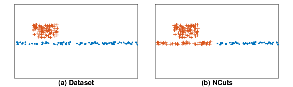
Spectral clustering aims to optimize certain criterion that measures the quality of graph partitions. For example, the NCuts (Shi and Malik 2000) method minimizes the normalized cut between clusters, which measures the weights of inter-cluster edges. Conventionally, objects’ affinity is given by some distance-based similarity. For multi-scale data, which consists of object clusters of different sizes and densities, distance-based similarity is often ineffective in capturing the correlations between objects (Zelnik-Manor and Perona 2004; Nadler and Galun 2006). This leads to poor performance of spectral methods. For example, Fig. 2(a) shows a dense rectangular cluster located on top of a very sparse strip-shaped cluster. Objects at different ends of the strip-shaped cluster are far apart and hence their distance-based similarity is small. Fig. 2(b) shows the clustering given by NCuts, from which we see that the strip-shaped cluster is incorrectly segmented.
In (Li et al. 2018), the ROSC algorithm was proposed to address the multi-scale data issue in spectral clustering. The idea is to rectify a given distance-based similarity matrix by deriving a coefficient matrix that can better express the correlation among objects. Intuitively, each entry in represents how well an object characterizes another object , and two objects are considered highly correlated (and thus should be put into the same cluster) if they give similar characterization to other objects. The coefficient matrix is constructed based on the similarity matrix as well as a transitive -nearest-neighbor (TKNN) graph. Specifically, two objects and are connected in the TKNN graph if there exists an object sequence such that adjacent objects in the sequence are -nearest-neighbors of each other. For example, objects that are located at far ends of the strip-shaped cluster (Fig. 2) are connected by a chain of K-NN relations. An important property that was proven in (Li et al. 2018) is that the matrix has the grouping effect (Lu et al. 2012; Li et al. 2018), which states that if two objects are similar in terms of both and TKNN graph connectivity, their corresponding coefficient vectors in are also similar. Based on , ROSC constructs a new correlation matrix . The grouping effect of ensures that highly correlated objects are grouped together by applying spectral clustering on .
Besides expressing the correlation between objects of the same cluster, another important factor for correct clustering is to suppress the correlation between objects of different clusters. ROSC, however, focuses on enhancing the former by deriving a coefficient matrix that amplifies intra-cluster correlation; it does not promote the latter. Our objective is to study methods that deal with both factors. Specifically, our proposed algorithm CAST regularizes matrix so that it has grouping effect and it exhibits inter-cluster sparsity. By sparsity, we refer to the desired property that entries in the matrix that correspond to inter-cluster object pairs should be 0 or very small, hence the matrix is sparse.
One common approach to enforce sparsity is to apply regularization on a solution matrix (i.e., by including the -norm as a penalty term in an optimization problem). While using the -norm helps sparsify inter-cluster correlation, it weakens intra-cluster correlation and hence it goes against establishing grouping effect. In contrast, ROSC uses the Frobenius norm to regularize the coefficient matrix , which is equivalent to regularizing each column vector of by the -norm. The Frobenius norm has been shown to enhance grouping effect but not sparsity. Generally, a desired coefficient matrix should possess both grouping effect for objects in the same cluster and sparsity for objects from different clusters. To construct such a matrix, we introduce trace Lasso (Grave et al. 2011), which is a regularizer that falls in between the -norm and the -norm. The trace Lasso is adaptive depending on the correlation between objects. Given a set of objects , let denote the feature matrix of objects, whose -th column is the feature vector of an object . (We assume the vectors are normalized, i.e., for all .) If objects are highly correlated, i.e., (1 is the all-one vector), the trace Lasso is equivalent to the -norm; If objects are independent, i.e., ( is the identity matrix), the trace Lasso will behave like the -norm.
In this paper we study spectral clustering over multi-scale data. We propose the Correlation-based Adaptive Spectral clustering method using Trace lasso, or CAST. We discuss how CAST takes advantage of the trace Lasso to achieve robust spectral clustering. We summarize our main contributions as follows.
We study the problem of applying spectral clustering on multi-scale data. We propose the CAST algorithm, which uses trace Lasso to construct and regularize a coefficient matrix . A correlation matrix that exhibits grouping effect and inter-cluster sparsity is subsequently derived for effective and robust spectral clustering.
We mathematically prove that the derived matrix by CAST has grouping effect. This ensures high intra-cluster object correlation.
We conduct extensive experiments to show the effectiveness of CAST. We compare CAST with 10 other methods w.r.t. various clustering quality measures over a wide range of datasets. Our results show that CAST consistently provides very good performance over the range of datasets. It is thus a very robust algorithm especially in handling multi-scale data.
The rest of the paper is organized as follows. Section 2 introduces related works. In Section 3 we describe the ROSC algorithm, give formal definitions of some important concepts based on which our algorithm is designed, and then present CAST. Section 4 presents experimental results. Finally, Section 5 concludes the paper.
2. Related Work
Spectral clustering is a widely studied topic (Bojchevski et al. 2017; Correa and Lindstrom 2012; Li et al. 2007; Chen et al. 2018; Xiang and Gong 2008). There are many works that study various aspects of spectral clustering, such as computational efficiency (Chen and Cai 2011; Cullum and Willoughby 2002; Yan et al. 2009), clustering performance on data with different characteristics (Huang et al. 2009; Von Luxburg et al. 2008; Zhu et al. 2014), and the theoretic foundations of the method (Lafon and Lee 2006; Nadler et al. 2005; Meila and Shi 2001). An introduction to spectral clustering is given in (Von Luxburg 2007; Kannan et al. 2004; Ng et al. 2001).
Despite the success of spectral clustering, previous works (Nadler and Galun 2006; Ye et al. 2016) have pointed out that spectral methods can be adversely affected when data is multi-scale. To address the problem, the self-tuning spectral clustering method ZP (Zelnik-Manor and Perona 2004) uses local scaling to extend a Gaussian kernel based similarity to , where (boldface) denotes the feature vector of an object , and is a scaling parameter. The original formulation uses a global scaling parameter for every object pair, which is difficult to set. When is set small, is small and it cannot effectively capture the high correlation between distant objects in a large sparse cluster. On the contrary, when is set large, is large. Objects from different but nearby dense clusters will then more likely to be mis-judged as similar. To address the issue, ZP introduces a local scaling parameter for each object , which is defined as the distance between and its -th nearest neighbor ( can be empirically set). For an object in a sparse cluster, is large. This enlarges the similarity between and other distant objects in the same cluster of . Also, a dense cluster gives a small , which effectively decreases the similarity between and objects from nearby clusters.
Other previous works (Alpert and Yao 1995) have suggested to use more eigenvectors to capture more cluster separation information to improve the effectiveness of spectral clustering on multi-scale data. There are methods that employ pseudo-eigenvectors generated by the power iteration (PI) technique. The PI method is used to compute the dominant eigenvector of a matrix. Lin et al. (Lin and Cohen 2010) point out that one can truncate the iterative PI process to obtain an intermediate pseudo-eigenvector. The pseudo-eigenvector is a weighted linear combination of all the eigenvectors and thus contains rich cluster separation information. They propose the Power Iteration Clustering (PIC) method based on the idea. Under PIC, however, each object has only one feature value given by the lone pseudo-eigenvector. When the number of clusters is large, a single pseudo-eigenvector is not enough to handle the cluster collision problem (Lin 2012). The PIC- method (Lin 2012) is subsequently proposed to address this issue. PIC- runs PI multiple times to generate multiple pseudo-eigenvectors. These pseudo-eigenvectors provide more features of objects for more effective clustering. One issue of the PIC- method is that the pseudo-eigenvectors are not orthogonal and thus are redundant. To reduce redundancy, (The et al. 2013) proposes a Deflation-based Power Iteration Clustering (DPIC) method that uses Schur complement to generate orthogonal pseudo-eigenvectors. Another issue of the PIC-based methods is that the more dominant eigenvectors are assigned larger weights in the PI iteration. Generally, they overshadow other lesser but indispensable eigenvectors. To address this issue, the Diverse Power Iteration Embedding (DPIE) method (Huang et al. 2014) is proposed. When a new pseudo-eigenvector is generated in DPIE, information of previously generated pseudo-eigenvectors is removed from the new one. Ye et al. (Ye et al. 2016) put forward a Full Spectral Clustering (FUSE) method. It uses independent component analysis to rotate generated pseudo-eigenvectors and make them statistically independent. The most informative ones are used for clustering. Finally, in (Li et al. 2018), a spectral clustering algorithm for multi-scale data, ROSC, is proposed. Details of ROSC will be covered in the next section.
3. Algorithms
In this section we first outline the ROSC algorithm, which is the basis of our algorithm CAST. We define TKNN graph and grouping effect. Then, we discuss the effect of different regularization methods on the coefficient matrix , which is constructed to derive object correlation. After that, we present CAST and prove that the matrix CAST derives has grouping effect and that it promotes sparsity.
3.1. ROSC
The basic idea of ROSC is to construct a coefficient matrix from a given similarity matrix and then perform spectral clustering based on . To construct , ROSC first applies PI multiple times to generate pseudo-eigenvectors. Whitening (Kessy et al. 2017) is used to reduce the redundancy of these pseudo-eigenvectors. The pseudo-eigenvectors together form a matrix . The -th column of is taken as the feature vector of an object . That is, ROSC takes the pseudo-eigenvectors as low dimensional embeddings of objects. Assuming the linear subspace model (Liu et al. 2013), ROSC characterizes each object by others with
| (1) |
where denotes a coefficient matrix such that each entry describes how well an object characterizes another object , and is a matrix that captures the noise in the pseudo-eigenvectors. The more similar two objects are, the more likely one object can be represented by the other.
To correlate objects that are located at far ends of a cluster, ROSC regularizes by a TKNN graph.
Definition 1.
(Transitive -nearest-neighbor (TKNN) graph) Given a set of objects , the TKNN graph is an undirected graph, where is the set of vertices and is the set of edges. Specifically, the edge (, ) iff there exists a sequence <> such that adjacent objects in the sequence are -nearest-neighbors of each other. We use a reachability matrix to represent the TKNN graph, whose (,)-entry if (, ) ; 0 otherwise.
ROSC optimizes the objective function
| (2) |
where the first term reduces noise , the second term is the Frobenius norm of and the third term regularizes by the TKNN graph. It is shown in (Li et al. 2018) that Eq. 2 has a closed-form solution that has the following grouping effect.
Definition 2.
(Grouping effect). Given a set of objects , let denote the -th column of . Assume that objects’ features are normalized, i.e., , . Let denote the conditions: (1) and (2) . A matrix is said to have grouping effect if
Grouping effect considers both feature similarity and reachability similarity of objects. Feature similarity is measured based on the closeness of objects’ feature vectors (columns in ), while reachability similarity is evaluated by columns in that express the connectivity of objects in the TKNN graph. Since the optimal solution has grouping effect, highly correlated objects in both similarities will have similar coefficient vectors in . ROSC will thus group the objects in the same cluster. Note that may be asymmetric and contain negative values. ROSC derives a correlation matrix and uses that as input to standard spectral clustering in place of the original similarity matrix .
3.2. Sparsity
ROSC focuses on generating a coefficient matrix that has grouping effect so that highly correlated objects have similar vector representations in . For effective clustering, we also require that objects from different clusters have sparse connections. To enforce sparsity, a common approach is to use regularization. We thus modify Eq. 2 as
| (3) |
where the second term is the -norm of . To avoid self-representation of objects, we further add the constraint , where is the main diagonal vector of . The optimization problem in Eq. 3 is convex and it is equivalent to solving the problem:
| (4) |
where returns a diagonal matrix whose main diagonal vector is that of . Eq. 4 can be solved by the inexact Augmented Lagrange Multiplier (ALM) method (Zhang 2010; Lin et al. 2010), which minimizes the following augmented Lagrangian function:
where is the Lagrangian multiplier and is a penalty parameter. can be minimized by alternatively updating one variable with the others fixed. To update , we set and derive
| (5) |
To update , we set and derive
| (6) |
where is the shrinkage-thresholding operator acting on each entry of a given matrix, which is defined as . The operator returns the argument value if it is non-negative; 0 otherwise. The operator gives the sign of the argument value. Algorithm 1 in Appendix shows the algorithm that uses inexact ALM to generate a sparse coefficient matrix . By the theory of inexact ALM, the convergence of Algorithm 1 is guaranteed (Lin et al. 2010).
3.3. CAST
Although the coefficient matrix derived with regularization (Eq. 3) has sparse entries for uncorrelated objects, the regularization also weakens the connections between correlated objects, which goes against the grouping effect. To construct a matrix with both grouping effect for highly correlated objects and sparsity for uncorrelated ones, we regularize by the trace Lasso, which is a regularizer that takes object correlation into consideration. Let be a feature matrix whose -th column is the feature vector of an object . We normalize such that , . Let be the coefficient vector (a vector in the coefficient matrix ) that corresponds to an object , the trace Lasso of is defined as
| (7) |
where is the diagonal matrix with as its main diagonal. The integration of into the norm distinguishes the trace Lasso from other commonly used norms like the -norm and the -norm. Note that,
| (8) |
where ’s are vectors of canonical basis. Consider as an encoding of object correlation. Then, if objects are uncorrelated, i.e., , the trace Lasso equals the -norm due to the orthogonality of and :
| (9) |
On the other hand, if all the objects are highly correlated and have the same feature vector , i.e., , the trace Lasso is equivalent to the -norm:
| (10) |
For other cases, the trace Lasso falls in between the - and the - norms:
| (11) |
Due to this adaptability, we apply the trace Lasso to regularize in Eq. 2. Specifically, given an object , we optimize:
| (12) |
The optimization problem is convex and can be solved by the inexact ALM method. We first transform the problem into:
| (13) |
The augmented Lagrangian function of Eq. 13 is
where , and are Lagrangian multipliers, and is a penalty parameter. We adopt an alternative strategy to update variables of as in Sec. 3.2 and the update rules are as follows:
| (14) |
Here, we overload the notation , which returns a diagonal matrix whose main diagonal is that of the argument matrix. Also, returns the main diagonal vector of the argument matrix.
| (15) |
| (16) |
Furthermore, updating is equivalent to solving the sub-problem:
| (17) |
which is convex and has a closed-form solution that can be solved by the Singular Value Thresholding (SVT) operator (Cai et al. 2010). Suppose the singular value decomposition of a rank- matrix , where and is the -th largest singular value. Let and . The solution to Eq. 17 is:
| (18) |
Algorithm 2, which is summarized in Appendix, shows the procedure for solving Eq. 12. It is pointed out in (Zhang 2010; Liu et al. 2013) that the convergence of inexact ALM cannot be generally proved when there are three or more variables. However, the convexity of the Lagrangian function guarantees convergence to some extent (Liu et al. 2013). Moreover, there are ways to ensure convergence, e.g., by observing that is upper bounded by Step 10 of Alg. 2. While it is difficult to prove the convergence theoretically, inexact ALM has been empirically observed to perform well in practice (Zhang 2010).
3.4. Grouping Effect
Previous works (Hu et al. 2014; Lu et al. 2013; Li et al. 2018; Lu et al. 2012) have shown that spectral clustering is effective when applied to data with grouping effect. As we defined in Def. 2, with grouping effect, if two objects are highly correlated, their characterizations of other objects are similar. We measure object correlation by both a feature similarity and a reachability similarity. We next prove that the coefficient vectors ’s regularized by the trace Lasso (Eq. 12) result in grouping effect.
Lemma 3.
Given , let . The optimal solution to the problem: , satisfies , . Moreover, if , then, , .
Proof.
The Lagrangian function of the problem can be written as: , where is the Lagrangian multiplier. By setting , we get . Since satisfies , we substitute into the equation and get , . If , then , i.e., . Hence, , . ∎
Given a set of objects , let denote the feature matrix of the objects and denote the optimal solution of Eq. 12. We rearrange as , where consists of column vectors that are similar to each other and consists of the remaining columns. In particular, satisfies:
where is a small positive value, is the all one’s vector and is the mean vector of columns of . Similarly, we rearrange . To prove has grouping effect, we only need to show that if , then , where is the average value of , is a positive value and . Formally,
Theorem 4.
Given a matrix and a vector , let be the optimal solution to the problem: . satisfies , and satisfies and . If , , where
and
The proof of Theorem 4 is given in the Appendix.
Theorem 5.
has grouping effect.
Proof.
Given two objects and in . When , will be close to and will be close to . Hence, . From Lemma 3, in Theorem 4 satisfies . If , we have and . Further, we get . According to Theorem 4, has to be very close to . As a result, given two highly correlated objects and such that , we have . thus has grouping effect. ∎
3.5. Clustering Procedure
Given a set of objects , we solve Eq. 12 for each object and construct an optimal solution for the coefficient matrix . To prevent self-representation, when we determine using Eq. 12, we remove the -th column vector from . We note that may be asymmetric and contain negative values. To fix, CAST computes a new matrix as in (Liu et al. 2013). It is easy to prove that , and thus all have grouping effect. Moreover, since the trace Lasso automatically self-adjusts to either the - or the - norm, enhances sparsity for objects of different clusters. (We will further illustrate this sparsity effect in the next section.) The matrix is then fed to the pipeline of a standard spectral clustering method (e.g., NCuts) in place of the original similarity matrix . Algorithm 3 in Appendix outlines CAST.
4. Experiment
In this section, we conduct extensive experiments to evaluate the performance of CAST. We compare CAST with 10 other clustering methods on a wide range of datasets w.r.t. three popular measures, namely, purity, adjusted mutual information (AMI), and rand index (RI). These measures evaluate the clustering quality with values in the range from 0 to 1. A larger value indicates a better clustering quality. For details of the three measures, see (Vinh et al. 2010; Lin and Cohen 2010). We include the experiment settings in the Appendix.
4.1. Algorithms for comparison
We group the algorithms into the following four categories.
(Standard spectral clustering methods): NCuts and NJW are two standard methods. They differ in the way they normalize the graph Laplacian, , where is a diagonal matrix with . NCuts uses the random-walk-based normalization while NJW employs the symmetric normalization .
(Power iteration (PI)-based methods): PIC, PIC-, DPIC, and DPIE apply PI to generate pseudo-eigenvectors as a replacement of eigenvectors. They were described in Section 2.
(Multi-scale-data-oriented methods): ZP and FUSE are two methods that are specifically designed to handle multi-scale data. They were discussed in Section 2. Note that ZP automatically estimates the number of clusters. For a fair comparison, we modify ZP so that it returns (the number of true) clusters.
(Matrix-reconstruction methods): This group includes ROSC and CAST. We also consider a version of ROSC that regularizes the matrix using the -norm instead of the Frobenius norm. (That is, we replace Eq. 2 by Eq. 3 and solve the optimization problem using Alg. 1.) We call the method ROSC with Sparse Matrix, or ROSC-S.
4.2. Performance results
[Synthetic datasets] We first use two synthetic datasets to illustrate the characteristics of the 11 methods. Both datasets consist of clusters with various densities and sizes. Fig. 4(a) shows Syn1, in which a sparse rectangular cluster (magenta) is sandwiched between a small dense circular cluster (yellow) and a large dense rectangular one (navy blue). The second dataset Syn2 is illustrated in Fig. 4(a), in which two dense square clusters are very close to a sparse half-ring cluster (red). In both datasets, an object in an elongated cluster can be closer to an object of another cluster than to an object that is at a far end of the same cluster. This is purposely done to make clustering very difficult and so that we can visually compare the matrix-reconstruction methods.
| Measure | NJW | NCuts | PIC | PIC- | DPIC | DPIE | ZP | FUSE | ROSC-S | ROSC | CAST |
|---|---|---|---|---|---|---|---|---|---|---|---|
| Purity | |||||||||||
| AMI | |||||||||||
| RI |
| Measure | NJW | NCuts | PIC | PIC- | DPIC | DPIE | ZP | FUSE | ROSC-S | ROSC | CAST |
|---|---|---|---|---|---|---|---|---|---|---|---|
| Purity | |||||||||||
| AMI | |||||||||||
| RI |


Tables 2 and 2 show the clustering performance of the methods for the datasets Syn1 and Syn2, respectively. From the tables, we see that matrix-reconstruction methods generally perform very well. For Syn1 (Table 2), w.r.t. Purity measure, ROSC, ROSC-S and CAST either perform better or comparably with the other methods. For measures AMI and RI, the matrix-reconstruction methods outperform others. For Syn2 (Table 2), CAST and ROSC outperform others by wide margins w.r.t. all three measures. ROSC-S has either better or comparable performance with other non-matrix-reconstruction methods. Moreover, CAST achieves the best performance over all three measures on both Syn1 and Syn2.
We visually compare the performance of the matrix-reconstruction methods for Syn1 in Fig. 4. Recall that ROSC-S uses the -norm to regularize the coefficient matrix. This promotes sparsity. However, as shown in Fig. 4(b), the sparse magenta cluster is incorrectly chipped off on the right side. In contrast, ROSC, which uses the Frobenius norm and promotes object correlation, is connecting objects aggressively. This causes some clusters to overspread into close neighboring clusters (see the regions enclosed in red boxes in Fig. 4(c)). From Fig. 4(d), we see that CAST rectifies the two problems by striking a balance between object connectivity and sparsity using the trace Lasso regularizer. This explains CAST being the best method for Syn1. Figs. 4(b), (c), (d) visually compare the three methods for Syn2. Again, ROSC-S promotes sparsity, and for Syn2, it inadvertently segments the half-ring cluster into three parts. ROSC, which promotes object correlation, recovers more objects of the half-ring cluster, but the half-ring is still split into three segments. For Syn2, CAST avoids the merging of objects on the right side of the half-ring cluster with the square cluster. This shows the adaptability of the trace Lasso regularizer.
Recall that the objective of the matrix-reconstruction methods is to construct a new matrix in place of the original similarity matrix and use the constructed matrix as input to the spectral clustering pipeline. Figs. 6 and 6 display the constructed matrices (together with the original similarity matrice ) for Syn1 and Syn2, respectively. Each figure displays values in a matrix by pixel brightness. Rows and columns in the matrix are reordered by gold-standard clusters. Readers are advised to view the figures magnified on a computer screen. Intuitively, each luminous rectangular block corresponds to a cluster. Ideally, a figure should have 3 blocks (because there are 3 clusters in each dataset); each block is brightly lit (showing high intra-cluster correlation); and pixels outside the blocks are black (showing sparse inter-cluster correlation).
From Figs. 6(a) and 6(a), we see that the original similarity matrices do not have the desired properties. In particular, pixels in blocks are sparse making the blocks not very visible. This results in poor clustering when spectral clustering is applied on directly. From Figs. 6(c) and 6(c), we see that by using the Frobenius norm, ROSC is able to significantly amplify intra-cluster correlations, resulting in brightly-lit blocks. However, inter-cluster correlations are inadvertently amplified as well, which is particularly striking in Fig 6(c). On the other hand, ROSC-S, which uses the -norm to promote sparsity, reduces inter-cluster correlation at the expense of less defined blocks. Finally, Figs. 6(d) and 6(d) show that CAST strikes a better balance between intra-cluster correlation and inter-cluster sparsity. This gives better-lit blocks with dimer regions outside the blocks compared with those of ROSC.
We further study how all 11 methods perform on multi-scale data by varying the densities and sizes of some clusters in the synthetic datasets. We make two changes: (1) increase the density of a cluster while keeping its size unchanged, and (2) increase the size of a cluster while maintaining its density unchanged. Here, we show some representative results. Specifically, we increase the density of the middle magenta cluster in Syn1 and use to denote the density change (e.g., = 20% means that the density of the cluster is 1.2 times larger than the original one). We change the size of the cluster by enlarging the length sideways with the height fixed. We use to denote the size change (e.g., = 100% means that the size of the cluster is doubled). We make similar changes to the half-ring cluster of Syn2. In particular, we gradually enlarge the size of the cluster from a half ring (, = 0%) to a whole ring (, = 100%). The clustering results are shown in Fig. 7. From the figure, we see that CAST gives the best and the most stable performances among all the methods over all the test cases. This shows that a similarity matrix with intra-cluster correlation and inter-cluster sparsity contributes positively to the clustering of multi-scale data. In contrast, ROSC-S, which constructs a sparse matrix but reduces connections between highly correlated objects, and ROSC, which computes a matrix with grouping effect but amplifies the inter-cluster correlations, are thus much less robust.


| Dataset | NJW | NCuts | PIC | PIC- | DPIC | DPIE | ZP | FUSE | ROSC-S | ROSC | CAST |
|---|---|---|---|---|---|---|---|---|---|---|---|
| COIL20 | |||||||||||
| glass | |||||||||||
| MNIST0127 | |||||||||||
| isolet_5class | |||||||||||
| Yale_5class |
| Dataset | NJW | NCuts | PIC | PIC- | DPIC | DPIE | ZP | FUSE | ROSC-S | ROSC | CAST |
|---|---|---|---|---|---|---|---|---|---|---|---|
| COIL20 | |||||||||||
| glass | |||||||||||
| MNIST0127 | |||||||||||
| isolet_5class | |||||||||||
| Yale_5class |
| Dataset | NJW | NCuts | PIC | PIC- | DPIC | DPIE | ZP | FUSE | ROSC-S | ROSC | CAST |
|---|---|---|---|---|---|---|---|---|---|---|---|
| COIL20 | |||||||||||
| glass | |||||||||||
| MNIST0127 | |||||||||||
| isolet_5class | |||||||||||
| Yale_5class |


[Real datasets] We further compare the methods using 5 real datasets. They are: COIL20 (images), glass (UCI repository), MNIST0127 (hand-written digit images), isolet_5class (speech, UCI repository), and Yale_5class (facial images). Some statistics of these datasets are given in the Appendix.
Tables 5, 5 and 5 show the performance results. Since we evaluate the methods on 5 datasets w.r.t. 3 measures, there are in total 15 “contests”. Each row in the tables corresponds to one contest. We highlight the winner’s score of each contest in bold. We also give the ranking of CAST in each contest next to its score. From the tables, we make the following observations:
Matrix-reconstruction methods (ROSC, ROSC-S and CAST) win in all but one contest (AMI-glass). In this case, CAST’s score (0.3390) is very close to that of the winner NJW (0.3469). This shows that matrix-reconstruction methods are superior in dealing with multi-scale data. Compared with other competitors, these methods derive new matrices that can more effectively capture object correlations, which explains their excellent performance. For example, all the three methods significantly outperform the rests for COIL20.
ROSC and ROSC-S each win in 5 and 6 contests, respectively. We also observe that there are quite a few cases in which their performances differ significantly. For example, ROSC-S beats ROSC 0.8038 to 0.7518 in AMI-isolet_5class, while ROSC outperforms ROSC-S 0.5822 to 0.5497 in Purity-glass. This is because ROSC lacks sparsity for inter-cluster connections while ROSC-S loses grouping effect for highly correlated objects. The results thus show that the relative performance of ROSC-S and ROSC varies across datasets. They are thus relatively unstable in their performance.
CAST provides a more stable performance across the datasets compared with ROSC and ROSC-S. First, CAST wins in 9 contests and ranks 2nd in 5 others. For the case that CAST is not top-2 (e.g., AMI-glass), it is the best algorithm among the matrix-reconstruction methods. With regularization using the trace Lasso, CAST takes advantage of both grouping effect and sparsity. It is thus more robust when applied to multi-scale data of different characteristics.
We end this section with a parameter analysis. CAST uses two parameters and to control the trace Lasso regularization term and the TKNN graph regularization term, respectively. We fix one parameter and vary the other. Fig. 8 shows the parameter analysis on the datasets isolet_5class and Yale_5class. From the figure, we see that CAST gives very stable performance over a wide range of parameter values.
5. Conclusions
In this paper, we studied the performance of spectral clustering on data with various sizes and densities. We reviewed existing spectral methods in handling multi-scale data. In particular, we observed that the ROSC algorithm constructs a matrix with grouping effect, but it fails to weaken connections between clusters. We thus proposed the CAST algorithm, which uses trace Lasso to balance the effect of and regularizations. We mathematically proved that the matrix constructed by CAST has grouping effect. We also show that the matrix achieves sparsity for uncorrelated objects. We conducted extensive experiments to evaluate CAST’s performance and compared CAST against other competitors using both synthetic and real datasets. Our experimental results showed that CAST performed very well against its competitors over all the datasets. It is thus robust when applied to multi-scale data of different properties.
6. Acknowledgments
This research is supported by Hong Kong Research Grants Council GRF HKU 17254016.
References
- (1)
- Alpert and Yao (1995) Charles J Alpert and So-Zen Yao. 1995. Spectral partitioning: the more eigenvectors, the better. In Proceedings of the 32nd annual ACM/IEEE Design Automation Conference. ACM, 195–200.
- Bojchevski et al. (2017) Aleksandar Bojchevski, Yves Matkovic, and Stephan Günnemann. 2017. Robust Spectral Clustering for Noisy Data: Modeling Sparse Corruptions Improves Latent Embeddings. In KDD. 737–746.
- Cai et al. (2010) Jian-Feng Cai, Emmanuel J Candès, and Zuowei Shen. 2010. A singular value thresholding algorithm for matrix completion. SIAM Journal on optimization 20, 4 (2010), 1956–1982.
- Chen and Cai (2011) Xinlei Chen and Deng Cai. 2011. Large Scale Spectral Clustering with Landmark-Based Representation. In AAAI. 313–318.
- Chen et al. (2018) Xiaojun Chen, Weijun Hong, Feiping Nie, Dan He, Min Yang, and Joshua Zhexue Huang. 2018. Spectral clustering of large-scale data by directly solving normalized cut. In KDD. ACM, 1206–1215.
- Correa and Lindstrom (2012) Carlos D Correa and Peter Lindstrom. 2012. Locally-scaled spectral clustering using empty region graphs. In KDD. 1330–1338.
- Cullum and Willoughby (2002) Jane K Cullum and Ralph A Willoughby. 2002. Lanczos algorithms for large symmetric eigenvalue computations: Vol. I: Theory. SIAM.
- Dhillon (2001) Inderjit S Dhillon. 2001. Co-clustering documents and words using bipartite spectral graph partitioning. In KDD. 269–274.
- Grave et al. (2011) Edouard Grave, Guillaume R Obozinski, and Francis R Bach. 2011. Trace lasso: a trace norm regularization for correlated designs. In NeurIPS. 2187–2195.
- Hu et al. (2014) Han Hu, Zhouchen Lin, Jianjiang Feng, and Jie Zhou. 2014. Smooth representation clustering. In CVPR. 3834–3841.
- Huang et al. (2014) Hao Huang, Shinjae Yoo, Dantong Yu, and Hong Qin. 2014. Diverse power iteration embeddings and its applications. In ICDM. 200–209.
- Huang et al. (2009) Ling Huang, Donghui Yan, Nina Taft, and Michael I Jordan. 2009. Spectral clustering with perturbed data. In NeurIPS. 705–712.
- Kannan et al. (2004) Ravi Kannan, Santosh Vempala, and Adrian Vetta. 2004. On clusterings: Good, bad and spectral. JACM 51, 3 (2004), 497–515.
- Kessy et al. (2017) Agnan Kessy, Alex Lewin, and Korbinian Strimmer. 2017. Optimal whitening and decorrelation. The American Statistician (2017).
- Lafon and Lee (2006) Stephane Lafon and Ann B Lee. 2006. Diffusion maps and coarse-graining: A unified framework for dimensionality reduction, graph partitioning, and data set parameterization. TPAMI 28, 9 (2006), 1393–1403.
- Li et al. (2018) Xiang Li, Ben Kao, Siqiang Luo, and Martin Ester. 2018. ROSC: robust spectral clustering on multi-scale data. In WWW. 157–166.
- Li et al. (2019) Xiang Li, Ben Kao, Zhaochun Ren, and Dawei Yin. 2019. Spectral Clustering in Heterogeneous Information Networks. In AAAI. 4221–4228.
- Li et al. (2007) Zhenguo Li, Jianzhuang Liu, Shifeng Chen, and Xiaoou Tang. 2007. Noise robust spectral clustering. In ICCV. 1–8.
- Lin (2012) Frank Lin. 2012. Scalable methods for graph-based unsupervised and semi-supervised learning. Ph.D. Dissertation. Carnegie Mellon University.
- Lin and Cohen (2010) Frank Lin and William W Cohen. 2010. Power iteration clustering. In ICML. 655–662.
- Lin et al. (2010) Zhouchen Lin, Minming Chen, and Yi Ma. 2010. The augmented lagrange multiplier method for exact recovery of corrupted low-rank matrices. arXiv preprint arXiv:1009.5055 (2010).
- Liu et al. (2013) Guangcan Liu, Zhouchen Lin, Shuicheng Yan, Ju Sun, Yong Yu, and Yi Ma. 2013. Robust recovery of subspace structures by low-rank representation. TPAMI 35, 1 (2013), 171–184.
- Lu et al. (2013) Canyi Lu, Jiashi Feng, Zhouchen Lin, and Shuicheng Yan. 2013. Correlation adaptive subspace segmentation by trace lasso. In ICCV. 1345–1352.
- Lu et al. (2012) Can-Yi Lu, Hai Min, Zhong-Qiu Zhao, Lin Zhu, De-Shuang Huang, and Shuicheng Yan. 2012. Robust and efficient subspace segmentation via least squares regression. In ECCV. 347–360.
- Meila and Shi (2001) Marina Meila and Jianbo Shi. 2001. A random walks view of spectral segmentation. (2001).
- Nadler and Galun (2006) Boaz Nadler and Meirav Galun. 2006. Fundamental limitations of spectral clustering. In NeurIPS. 1017–1024.
- Nadler et al. (2005) Boaz Nadler, Stephane Lafon, Ronald Coifman, and Ioannis Kevrekidis. 2005. Diffusion maps, spectral clustering and eigenfunctions of Fokker-Planck operators. In NeurIPS. 955–962.
- Ng et al. (2001) Andrew Y Ng, Michael I Jordan, Yair Weiss, et al. 2001. On spectral clustering: Analysis and an algorithm. In NeurIPS. 849–856.
- Shi and Malik (2000) Jianbo Shi and Jitendra Malik. 2000. Normalized cuts and image segmentation. TPAMI 22, 8 (2000), 888–905.
- The et al. (2013) Anh Pham The, Nguyen Duc Thang, La The Vinh, Young-Koo Lee, and Sungyoung Lee. 2013. Deflation-based power iteration clustering. Applied Intelligence 39, 2 (2013), 367–385.
- Vinh et al. (2010) Nguyen Xuan Vinh, Julien Epps, and James Bailey. 2010. Information theoretic measures for clusterings comparison: Variants, properties, normalization and correction for chance. JMLR 11 (2010), 2837–2854.
- Von Luxburg (2007) Ulrike Von Luxburg. 2007. A tutorial on spectral clustering. Statistics and computing 17, 4 (2007), 395–416.
- Von Luxburg et al. (2008) Ulrike Von Luxburg, Mikhail Belkin, and Olivier Bousquet. 2008. Consistency of spectral clustering. The Annals of Statistics (2008), 555–586.
- Xiang and Gong (2008) Tao Xiang and Shaogang Gong. 2008. Spectral clustering with eigenvector selection. Pattern Recognition 41, 3 (2008), 1012–1029.
- Yan et al. (2009) Donghui Yan, Ling Huang, and Michael I Jordan. 2009. Fast approximate spectral clustering. In KDD. 907–916.
- Ye et al. (2016) Wei Ye, Sebastian Goebl, Claudia Plant, and Christian Böhm. 2016. FUSE: Full Spectral Clustering. In KDD. 1985–1994.
- Yu and Shi (2003) Stella X. Yu and Jianbo Shi. 2003. Multiclass spectral clustering. In ICCV. 313–319.
- Zelnik-Manor and Perona (2004) Lihi Zelnik-Manor and Pietro Perona. 2004. Self-tuning spectral clustering. In NeurIPS. 1601–1608.
- Zhang (2010) Yin Zhang. 2010. Recent advances in alternating direction methods: Practice and theory. In IPAM workshop on continuous optimization.
- Zhu et al. (2014) Xiatian Zhu, Chen Change Loy, and Shaogang Gong. 2014. Constructing robust affinity graphs for spectral clustering. In CVPR. 1450–1457.
Appendix A Experiment
A.1. Dataset statistics
We summarize the statistics of datasets used in our experiments in Table 6.
| Dataset | #objects | #dimensions | #clusters |
|---|---|---|---|
| COIL20 | |||
| glass | |||
| MNIST0127 | |||
| isolet_5class | |||
| Yale_5class |
A.2. Experiment settings
For all the datasets, the similarity matrix is computed based on Euclidean distance of objects’ attributes. is also locally scaled as is done in ZP. All the methods employ k-means as the last step of the clustering pipeline to return clusters. For this step, we run k-means times with random starting centroids and the most frequent cluster assignment is used (Lin and Cohen 2010). For ROSC, ROSC-S and CAST, we set in constructing the TKNN graph as suggested in (Li et al. 2018), and fine tune the parameters by grid search for to report the best results. For other methods, parameters are set according to their original papers. For each method and dataset, we run the experiment 50 times and report average results. Our codes and datasets are publicly available at https://github.com/lixiang3776/CAST.
Appendix B Algorithms
We give the details of the pseudocodes. Algorithm 1 and 2 introduce solving Eq. 3 and Eq. 12 by inexact ALM, respectively. Algorithm 3 summarizes CAST.
Appendix C Proof
In this section we prove Theorem 4. We first consider two lemmas.
Lemma 1.
Given , , .
Lemma 2.
If , , and , then .
For proofs of both lemmas, see (Lu et al. 2013). Next, we prove Theorem 4. Let . We get