Mesh quality preserving shape optimization using nonlinear extension operators
Abstract
In this article, we propose a shape optimization algorithm which is able to handle large deformations while maintaining a high level of mesh quality. Based on the method of mappings we introduce a nonlinear extension operator, which links a boundary control to domain deformations, ensuring admissibility of resulting shapes.
The major focus is on comparisons between well-established approaches involving linear-elliptic operators for the extension and the effect of additional nonlinear advection on the set of reachable shapes.
It is moreover discussed how the computational complexity of the proposed algorithm can be reduced.
The benefit of the nonlinearity in the extension operator is substantiated by several numerical test cases of stationary, incompressible Navier-Stokes flows in 2d and 3d.
AMS subject classifications: 35Q93, 49Q10, 35R30, 49K20, 65K10
Keywords: Aerodynamic shape optimization, method of mappings, nonlinear extensions
1 Introduction
Shape optimization is a discipline in the field of optimization constrained by partial differential equations (PDEs). Here the contour of the domain , where typically a PDE models the effects of interest, plays the role of the optimization variable. Possible variants are that the outer shape of is to be determined, e.g. when represents a solid body, or interior interfaces, which separate spatially discontinuous coefficients such as material properties. Shape optimization in general is nowadays an active field of research with applications ranging from electrostatics [22], interface identification in transmission processes [27, 10, 21], fluid-dynamics [25, 2, 7], acoustics [31], image restoration and segmentation [12] and composite material identification [28, 23] to nano-optics [13].
In this article, we focus on shape optimization in fluid dynamics, which is also one of the pioneering applications in this field [19, 15, 9]. In general, the optimization problem can be formulated as
| (1) | ||||||
where is a shape functional depending on a state variable and the shape of the domain . Moreover, fulfills the PDE constraint , which itself depends on . A typical example is an obstacle specimen in a flow tunnel as depicted in figure 1. One of the main questions is an appropriate choice of the set of admissible shapes , in which optimization takes place. For problems of this type, two prominent approaches can be identified in the literature. On the one hand, the Hadamard-Zolésio structure theorem is applied, which allows to trace back changes in the objective solely to variations of the boundary (see for instance [30, 18]). It is thus possible to define directional shape derivatives via variations of in a direction normal to the boundary. Together with the choice of an appropriate shape and tangent space, this allows to represent the sensitivity for w.r.t. as a gradient. This is then interpreted as a deformation to and a new discretization mesh for the resulting domain can be computed. By this step the mesh quality of the deformed domain can be ensured as pursued in, e.g., [32, 5]. Alternatively, the definition of shape and tangent space includes the surrounding domain , which immediately results in deformation information for the entire mesh (e.g. [22, 26, 6]) and makes the additional call to a mesh generator superfluous. Typical approaches consider interpreting the shape sensitivity as a force term in linear elastic models described over . The resulting displacement field is then applied as a mesh deformation. Especially in recent works (see for instance [11, 3, 4]), linear elastic extension equations are considered and, in particular, a very small or even zero first Lamé constant is favored.
Moreover, a descent method allows to control the mesh quality from one iteration to the next, i.e. for one deformation. Yet, in the limit of the sequence of design updates, quality is typically lost. This effect is described in, e.g., [23], where variable interfaces must be prevented from overlapping.
In this article we follow a different approach, which gives a higher level of control on the quality of the mesh around the optimal shape. Based on the method of mappings (cf. to [20]), the question for admissible shapes in equation 1 is translated to the choice of appropriate function spaces, in which a deformation from reference to the optimal configuration is to be found. Here denotes a set of admissible mappings. Starting from a reference configuration , it is then optimized over the transformations yet without explicitly performing mesh deformations. For this purpose the PDE constrained is transformed to the virtual domain as . The optimization problem then turns into a classical optimal control in the form of
| (2) | ||||||
This approach is a recent field of studies and applied in, e.g., [17, 29, 2]. Also based on this approach is the investigation in [11], which is the starting point for the consideration in the present article. Here the problem in equation 2 is formulated as
| (3) | ||||||
in terms of a regularization parameter and a bound on the determinant of the derivative of the mapping function . The focus of the investigations therein is on the extension operator . It is suggested to choose to be the composition of mappings . Here is realized via the solution operator of a Laplace-Beltrami equation on . The mapping to the actual displacement, i.e. , is then chosen to be the solution operator of a vector-valued elliptic equation, such as a linear elastic model. It is proven that – under certain circumstances – the domain mapping is locally a -diffeomorphism provided that is fulfilled.
The main focus of our present article is a numerical study of different choices of the extension operator . It turns out that optimization settings, where larger deformations are to be expected, are a limiting factor for linear operators .
This limitation is due to the fact that the structure of a shape space, that is as large as possible, can hardly be linear since this would require to explain what scalar multiples or sums of shapes are. Yet, with the method of mappings and a linear extension operator we approximate the set of admissible shapes locally by a linear function space of admissible deformations to a reference configuration.
We thus suggest a nonlinear extension mapping and present numerical studies on the applicability. It should be mentioned that the theory developed so far is not applicable in this case. It only applies to the linear choice of , which is a special case of the more general consideration in this article.
The motivation for the choice of in this present work is the observation that, on the one hand, via the condition the local injectivity of can be ensured. But on the other hand, this limits significantly the subset of admissible transformations and thus affects optimal shapes as outlined in the last section of this article. It is thus the task to find an operator which prevents from becoming active even for large deformations. We also discuss cases where the reference domain is not of circular shape and demonstrate the performance of the extension and influence on the mesh quality in a deformed domain. The intention of this experiment is to demonstrate that the set of shapes , which is constructed via the mappings from , can be extended significantly and the dependence on the choice of a reference domain can be hidden. In particular, the studies illuminate whether large deformations in the optimization are possible for general reference configurations, which do not fulfill certain properties like convexity or an injective normal vector field.
This article is structured as follows: In section 2 the shape optimization problem is set up and formulated in terms of the method of mappings. Section 3 is devoted to the nonlinear extension model and, furthermore, the derivation of necessary optimality conditions and the presentation of an optimization algorithm. In section 4 numerical studies are conducted and discussed. The article closes in section 5 with a conclusion of the results.
2 Optimization problem
We carry out our considerations based on a classical optimization problem in the field of fluid dynamics described in [19]. In a -dimensional, bounded domain with Lipschitz boundary, as sketched in figure 1, we consider the minimization of the following energy dissipation functional
| (4) |
where the contour of the obstacle is assumed to be variable. The spatial dimension is chosen as . In equation 4 the velocity field denoted by is given in terms of the stationary, incompressible Navier-Stokes equations
| (5) | ||||||
Together with the fluid domain is allowed to change, but the outer boundaries, i.e. , and , of the experiment are fixed. In equation 5 denotes the pressure, describes the velocity profile at the inflow boundary, is the outer normal vector and the viscosity. Furthermore, we assume that holds during the entire optimization.
For the shape optimization of a specimen with respect to functionals of type equation 4, it is essential to exclude trivial solutions. Here, shrinking to a point or translations towards represents undesired descent directions. Thus, the optimization problem has to be additionally constrained to geometrical conditions. Our benchmark problem is to find optimal shapes of a specimen with a given volume, which remains located in the center of the flow tunnel. This is achieved by fixing barycenter and volume of the obstacle with the constraints
| (6) | ||||
| (7) |
Since the computation for the barycenter involves the volume of itself, these conditions are coupled in principle. Yet, if equation 6 is fulfilled, the term in equation 7 is constant and can thus be factored out. By further assuming that the barycenter of the specimen is , it is thus sufficient to require .
In the following, for a vector-valued function , we denote by the Jacobian matrix with the ordering . Let further
| (8) |
and consider the weak formulation of the PDE constraint equation 5:
Find such that
| (9) | ||||
for all test functions . Note that within this article we are using the symbol for test functions associated with a given variable.
In order to reformulate the optimization problem equations 4 to 7 as an optimal control problem in appropriate function spaces, we consider from now on the domain as a fixed reference configuration. Let with such that results in an admissible deformation for . For the method of mappings we then consider the state equation 9, objective equation 4 and the corresponding state variable in terms of .
By means of standard computations we obtain the weak formulation of the optimization problem pulled back to the reference domain by
| (10) | ||||
| s.t. | ||||
| (11) | ||||
| (12) | ||||
| (13) | ||||
| (14) |
for all test functions . The optimization problem equations 10 to 14 still leaves open the question for the set of admissible mappings . We thus follow the same approach as in [11] and translate it into the form of equation 3. By reformulating the constraint as a penalty term, we obtain the final optimal control problem
| (15) | ||||
where denotes the positive-part function. The missing piece is now mapping from a scalar-valued boundary control to admissible deformation fields , which is the subject of the next section.
3 Nonlinear extension operators
Consider the optimal control problem equation 15. The core of the reformulated shape optimization is the choice of the extension operator , which links a scalar-valued boundary control living on to a vector-valued displacement field in . A domain transformation mapping is then obtained by the so-called perturbation of identity. In particular, has to fulfill certain regularity properties as investigated in [11]. It yet turns out in section 4 that for large deformations, i.e. when the reference domain and the optimal configuration differ significantly, linear operators do not lead to satisfying results. Note that the choice of significantly influences the set of reachable shapes determined via . It is thus our intention to find which allows for large deformations without significantly restricting . Simultaneously, the corresponding mesh deformations should exhibit high element qualities for further usage in numerical simulations.
The focus of the present article is thus to propose and study nonlinear extensions given in terms of the solution operator of the coupled PDEs
| (16) | ||||||
In the equation above denotes the vector-valued Laplace-Beltrami operator. Note that by solving equation 16 the scalar-valued control is mapped to a vector valued quantity . The benefit of this particular extension operator, and especially the nonlinearity , which is in the focus of this article, becomes particularly visible for experiments with large deformations as pointed out in section 4.2. A popular choice, as discussed in the introduction, is to define the extension only via the linear term . Yet, this restricts the set significantly. This is visible especially for problems in fluid dynamics, as pointed out in section 4, where the reference shape is of spherical type but the optimum to be found is stretched and approximates non-smooth tip and back.
Problems arise due to strong compressions of finite elements in the discretization orthogonal to the main deformation direction. This observation motivates to add the nonlinear advection term , which – geometrically speaking – promotes displacements where nodes move along large gradients. This results in a homogeneous distribution of finite elements even around approximately non-smooth regions of .
For equation 16, which specifies the mapping from boundary control to domain deformation, the weak formulation is given by: Find such that
| (17) | ||||
| (18) |
for all and in terms of . Here denotes the derivative tangential to . In equation 17 the scalar-valued boundary control is multiplied with the outer normal vector field to at . Then a vector-valued Laplace-Beltrami equation is solved over . This is coupled with nonlinear equation 18 where the influence of the advection term is controlled via . Note that the linear extension operators investigated in [11] arise as a special case of system equations 17 and 18.
Now that the extension operator is chosen, we can combine the optimization problem equation 15 with the extension operator equations 17 and 18 to obtain the Lagrangian
| (19) |
where denotes for each variable the associated multiplier. Note that there is no variable corresponding to the multipliers and . These are the finite dimensional multipliers for the barycenter and volume condition equations 6 and 7.
Lemma 1.
The first order optimality system associated to the Lagrangian in equation 19 is given by the derivatives as
| (20) | ||||
| (21) |
| (22) | ||||
| (23) | ||||
| (24) |
| (25) |
| (26) |
| (27) |
| (28) |
| (29) |
| (30) |
for all test functions , , , , , , , , , , and .
Proof.
The derivatives of are obtained by utilizing standard rules of differentiation. Note that we particularly use the following identities
For the derivative of the penalty term we utilize that
∎
Recall that the condition in the problem formulated in equation 3 is realized via the penalty term . The corresponding term in equation 20 of the optimality system in lemma 1 is non-differentiable due to the positive-part function . Following the discussions in [11, sec. 3.5] the mapping is semismooth and one can compute an element from the generalized derivative in direction as
In the following we briefly present a solution algorithm for the optimality system equations 20 to 30. For this purpose we pursue a similar approach as in [11]. The core of this method is to solve the nonlinear shape optimization problem equation 15 for a decreasing sequence of regularization parameters , starting from until the desired level is reached. Because each subsequent optimization problem is nonlinear, this approach benefits from utilizing the known values as initial guess in the -th iteration. Algorithm 1 summarizes this procedure. Since parts of the optimality system are non-differentiable, we apply a semismooth Newton’s method.
In section 4 we demonstrate how to choose the paramter and and illustrate their influence.
4 Numerical results
This section is devoted to different numerical case studies of stationary, incompressible Navier-Stokes shape optimization problems. The purpose is to illuminate features of the nonlinear extension operator proposed in section 3. In particular, the benefit for optimization benchmark problems, which involve large deformations from the reference configuration to optimal shapes, is numerically investigated. It is moreover discussed how the local injectivity can be extended to globally injective transformation mappings by adding an artificial volume to the aerodynamic specimen. Furthermore, algorithmic solvability of the optimality system equations 20 to 30 is addressed in the end of this section.
The experimental settings for the tests are chosen to be comparable in 2d and 3d, respectively. The holdall domain , which reflects the flow tunnel in the experiment, is chosen as
Let denote the diameter of the flow tunnel . We then fix the velocity at the inflow boundary by . In all experiments where the specimen is a circle or sphere, the radius is given by and .
The discretization of all appearing PDEs is carried out with standard, piecewise linear P1 finite elements. In order to guarantee stability, we follow the pressure stabilized Petrov Galerkin approach (see for instance [14]), which utilizes an additional term for the pressure and its adjoint variable . The system under consideration is thus enriched by the two equations
where denotes the set of all finite elements and measures the longest edge of element . For each of the subsequent experiments, is chosen.
All computations related to the finite element method are carried out using the GETFEM++ library [24]. We utilize a parallel version of the library, which relies on PARMETIS [16] for mesh partitioning and load balancing. All linear systems are handled via the parallel factorization solver MUMPS [1]. Both, 2d and 3d discretization meshes are produced with the GMSH toolbox [8] and the Delaunay algorithms therein. If not stated otherwise, all 2d experiments follow the strategy of algorithm 1 with the choice , and .
4.1 Non-convex shapes with large deformations


Our first numerical study demonstrates the nonlinear extension equation for large deformations of a non-convex shape. The reference domain is chosen such that the specimen is described by a B-spline curve given in terms of 6 control nodes. The situation is depicted in figures 2 and 3.
The relevance of this test case is to investigate the performance of the proposed approach for reference domains where the normal vector field does not homogeneously point in all directions as for a circular shape. The influence of the normal vector is significant since it initially links the scalar-valued control to a vector-valued quantity as can be seen in equation 16. Section 4.3 is devoted to an experiment where several directions are underrepresented in the discretization of the normal vector due to the shape of .
In figure 2 the magnitude of velocity , computed in the undeformed state , i.e. when , is depicted. The right-hand side shows the velocity according to deformation in terms of the optimal control after solving the optimality system given by equations 20 to 30. Furthermore, the optimal mapping can be seen in figure 3 in the displacement and deformation of discretization elements. The relocation of triangles shows the effect of the nonlinear advection in the extension operator. A deeper look on this effect and the resulting mesh quality is provided in section 4.5.
In this experiment the viscosity of the fluid is chosen as . The holdall domain is as described above. It consists of surface segments on and triangles in . Barycenter and volume of in the reference configuration are given by and . Thus, an optimal shape also undergoes a small translation since is required.
The essential settings in terms of shape optimization are the parameter and . Here we choose , which leads to the condition with being inactive. We can explain the homogeneously and smoothly deformed mesh due to this fact. In contrast, section 4.2 shows examples where is active close to the tip of the optimal shape and how the displacement and thereby the mesh quality in is affected.
4.2 Influence of factors and
In this section we visualize the influence of the choice of and on the optimization. This demonstrates how the set of admissible shapes is determined thereby. The underlying experiment is a flow in over a circular specimen as described at the beginning of section 4. The viscosity is again chosen to be . The domain is discretized with segments on and triangles in .
First, we observe the influence of on the set of admissible shapes . Figure 4 visualizes how the condition acts on the optimal shape . Here we choose beginning with the largest and then decreasing values. This condition can be interpreted such that the allowed, local change of volume in is relaxed from top to bottom in figure 4. In this experiment it turns out that in the last computation with the condition is inactive. Here is fixed in all computations.
The next experiment follows the same setup with the only difference that is now fixed and takes increasing values. The mesh deformations, resulting from the optimal solution , are visualized in figure 5. Each of the subfigures shows a clip of size around the tip of the optimal shape. Besides the significantly improved mesh qualities and more adequate set we also observe that the Newton solver benefits from the appropriate choice of and . As soon as the condition becomes active, the optimality system equations 20 to 30 is not differentiable any further and the solver switches to semismooth Newton’s method. This effect is already documented in [11] for the case of Stokes flows and linear extension operator .
4.3 Extending the local-only injectivity


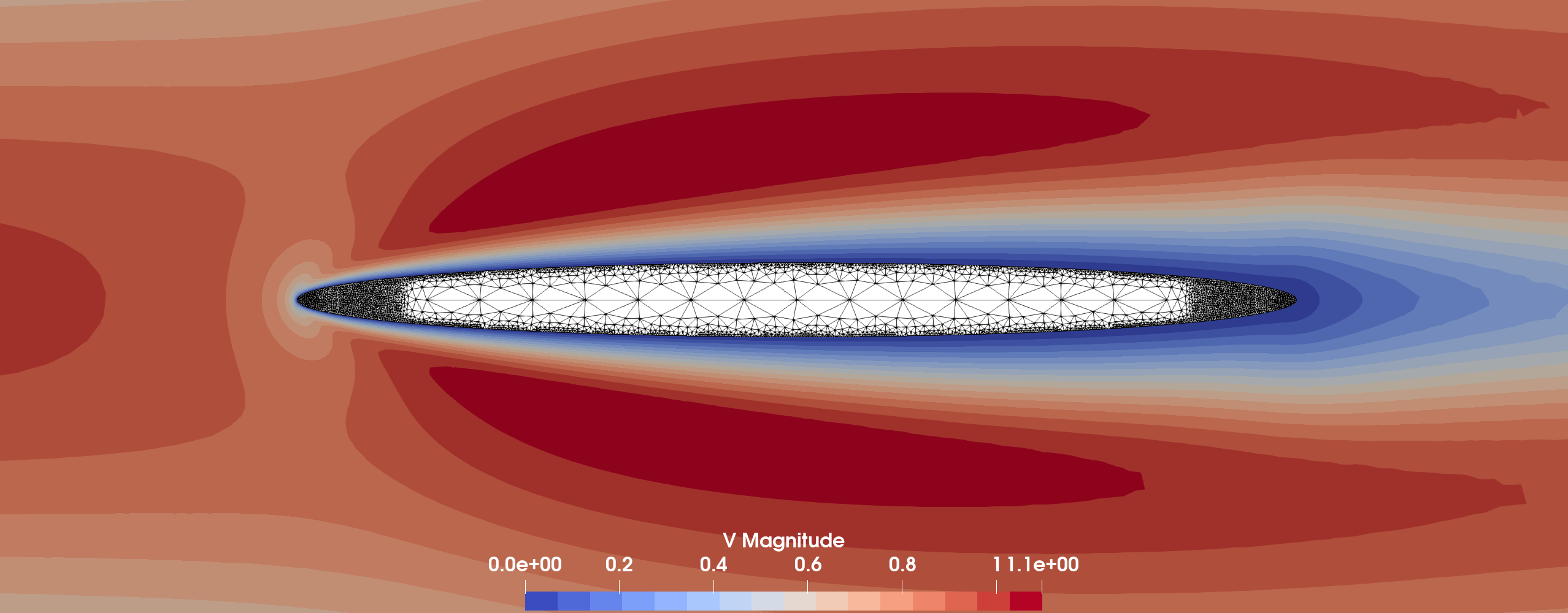

This section focuses on an effect that is likely to appear for non-spherical reference domains. In particular, for the aerodynamic experiments considered in this article it might happen that the upper surface of the obstacle overlaps the lower one. Especially for large deformations from reference to optimal shape and for shapes that are streched parallel to the flow axis, we encounter effects as depicted in figure 6(a) for the experiment shown in figure 7. In other words, is not globally injective in this situation. This is due to the fact that the condition ensures injectivity of only locally but not globally.
In the following we propose a modification of the extension operator in order to extend the injectivity. Recall that in the setting followed up to here the obstacle domain is treated as void and there is no discritization within. We now consider the operator on the entire holdall domain in contrast to the state equation that remains in . Moreover, the condition is now required on . Thus, the displacement field is defined by . Moreover, we reformulate the weak formulation of the extension operator given in equation 18 to
| (31) |
for all and appropriate . Simultaneously, the penalty term, which enforces the local injectivity, in equation 19 changes to
| (32) |
For this experiment we choose as in the previous sections. The holdall has the same outer dimension and the specimen is an ellipse with semimajor-axis , semiminor-axis and barycenter . Its surface is subdivided in segments. Further, is discretized by triangles, in and in .
Figure 6 visualizes the effect of the mapping on the discretization grid. In figure 6(a) the optimal solution for is shown. Note that in this particular case we stop the optimization for a larger value, since this already leads to singularities. Figure 6(b) depicts , which is again bound away from zero by . It can be seen that, although this condition is inactive, the non-injective mapping can not be prevented.
The same experiment is then conducted with the changes proposed in the beginning of this section, which leads to the values of shown in figure 6(c). Now is discretized and also acts on the interior of the specimen. Here the optimization is performed with the setting , and . The resulting optimal solution is visualized in figure 7 where figure 7(a) shows the reference domain and the velocity field computed for this configuration. Figure 7(b) depicts the domain and the velocity field computed on . Note that the relatively fine grid is chosen at the front and the back of the shape due to the large curvature of in these regions. This experiment turns out to be more challenging than, e.g., a spherical reference shape since on coarse grids the normal vector field in these areas tends to be underresolved. From a computational point of view, it is attractive to have a coarse grid in , as chosen in the center of the specimen, to reduce cost for the solution of the operator .
4.4 Three-dimensional results
In this section we perform a three-dimesional optimization experiment as a proof of concept. As already observed in [11] for the Stokes experiment, more care has to be taken for the decrease-strategy of in algorithm 1. Especially the semismooth Newton solver shows to be challenging w.r.t. to convergence when the condition becomes active.
The experiment shown in figure 8 is within the framework described at the beginning of section 4. The flow tunnel is discretized by tetrahedrons and the surface of the spherical specimen in the reference configuration consist of triangles. Further, the viscosity is chosen to be and in algorithm 1 we set , and . The results shown here are obtained with an extension factor of . We visualize the impact of the optimization on the fluid by stream lines of the velocity field in figure 8. This figure also shows the effect of the particular operator on the quality of the surface mesh when it undergoes the optimal deformation . The combination of Laplace-Beltrami equation 17 and the nonlinear extension equation equation 17 leads to a homogeneous distribution of triangles on the surface . It can be observed that this is due to tangential components in . This is a benefit of a vector-valued extension equation over approaches which utilize a static extension of the normal vector field in order to extend the boundary control to the surrounding volume. Furthermore, figure 9 shows a zoom-in to the tip of the deformed domain . Here we can see a crinkled clip in the -plane with , which shows the quality of the tetrahedrons.


4.5 Quantification of the influence of on mesh quality
This section presents numerical experiments which investigate the influence of the nonlinear extension operator on the mesh quality in 2d and 3d (cf. figure 10). Recall that the discretization mesh is not actually deformed within the optimization. We though deform the reference domain according to the optimal control and the corresponding deformation . The 2d experiment is conducted on the same computational domain as before with a circular specimen, surface segments and triangles in . The fluid viscosity is chosen to be . Figure 10 visualizes the influence of on the mesh quality of . It is measured by the ratio of radii of largest inscribed and smallest circumscribed circle, where the plot shows the value of the worst triangle.
This experiment quantifies the effect which is already visualized in figure 5. For a shape optimization with large deformations from reference to optimal configuration, i.e. is relatively large, a pure linear extension operator does not reliably lead to satisfying mesh qualities. Moreover, it can be seen that in this particular experiment there is a saturation effect of the nonlinearity in starting at approximately . Figure 10 shows the results of a similar experiment in 3d. Here a mesh is chosen with surface triangles on and tetrahedrons in . Note that we decrease the viscosity to in this experiment in order to be able to obtain results for . In 3d quality is measured by the radius ratio of smallest circumscribed sphere to the largest inscribed one. Again the worst element is visualized. Also note that the y-axis is in log-scale. In this setting it turns out, that the effect of compressed cells near the tip and back of the shape, which is stretching due to a decrease in , is stronger than in 2d. We explain the solver failure due to the semismoothness in the optimality system, which becomes active in a significant number of finite elements in this situation. However, it can be observed that, starting with approximately , a saturation is possible, where the mesh quality of remains adequate for further numerical computations.
4.6 An iterative optimization algorithm
In the previous sections we solve the nonlinear, non-smooth optimality system with the direct solution strategy given in algorithm 1. Moreover, a direct solver library is applied to the resulting linear systems within semismooth Newton’s method. This approach is clearly limited due to the high memory requirement. Especially, when the state equation results from a time-dependent problem, this procedure becomes impracticable. Hence, in this section we focus on a numerical study of decoupling system equations 20 to 30. This approach is summarized in algorithm 2.
We demonstrate that it is possible to decouple the solution process of state equations 23 and 25, adjoint equations 22 and 24 and shape related equations, i.e. equations 20, 21, 26, 27, 28, 29 and 30, from each other. On the one hand, this allows to reuse existing solvers for the state equation and embed them into the shape optimization framework. On the other, the memory requirement for linear solvers significantly reduces. Moreover, the semismooth part equation 20 is split from the other equations and a solver can be particularly tailored for this purpose.
Algorithm 2 operates on the nonlinear optimality system as a fixpoint strategy. In an outer loop it is again iterated over a decreasing regularization parameter as in algorithm 1. Thus, approximate solutions for the optimization problem according to are utilized as initial guess for the nonlinear solver in iteration . Yet, unlike in the direct approach, the subproblems are only solved approximately by a fixpoint iteration, which solves the decoupled equations of the optimalitiy system in turns. The termination criterion for this inner loop is the relative change in the control variable measured in the -norm.
In figure 11 the results of one run of algorithm 2 are shown. The underlying optimization experiment is a 2d computation on the same grid as in section 4.5 with surface segments and triangles in , , , , and . Note that the initial value of is significantly larger then the choices made for algorithm 1. Figure 11 shows the required inner iterations until the condition
is fulfilled for . Futhermore, the value of the objective (cf. equation 15) is visualized. It is computed in algorithm 2 in line 10 at the end of one inner loop. Notice the jumps in the objective function between iteration 5 and 20. In our experiments it turns out that this is an effect that both influences the minimal possible and .
In this setting a total number of 53 inner iterations, i.e. solutions of the state equation, are required to reach the optimal shape. This numerical study can thus be seen as a proof of concept how to reduce the computational costs of the large, coupled, nonlinear system equations 20 to 30. Thus, the proposed method is applicable to more complex problems, such as non-stationary Navier-Stokes flows.
5 Conclusion
In this article we have proposed and numerically demonstrated choices of nonlinear extension operators within the method of mappings for aerodynamic shape optimization. These operators are based on the idea that an additional, nonlinear advection term leads to a rearrangement of discretization cells along the major direction of deformations.
The main goal we have achieved is to circumvent mesh degeneracy effects that appear under large deformations when the extension of the boundary control is chosen according to linear elastic models. Especially in the underlying aerodynamic drag minimization, where optimal shapes tend to become stretched in flow direction and compressed in the orthogonal directions, we have numerically investigated how mesh quality can be preserved.
We have also demonstrated one possibility to decouple the solution process of the optimality system in order to overcome issues of computational complexity. Moreover, we have studied how the set of admissible shapes depends on the nonlinearity of the operator and how the local injectivity of mappings can be extended to large deformations. Since the proposed methodology is formulated in function spaces without taking a specific discretization into account, another benefit of this approach is that it naturally allows to introduce concepts like adaptivity. An important field for future investigations is a detailed description of properties of the set , which is constructed in terms of the nonlinear extension operator .
Acknowledgment
The work of the authors has been supported by the Deutsche Forschungsgemeinschaft (DFG, German Research Foundation) within the Research Training Group 2583 “Modeling, Simulation and Optimization of Fluid Dynamic Applications”.
References
- [1] P.. Amestoy, A. Guermouche, J.-Y. L’Excellent and S. Pralet “Hybrid scheduling for the parallel solution of linear systems” In Parallel Computing 32.2, 2006, pp. 136–156
- [2] C. Brandenburg, F. Lindemann, M. Ulbrich and S. Ulbrich “A Continuous Adjoint Approach to Shape Optimization for Navier Stokes Flow” In Optimal Control of Coupled Systems of Partial Differential Equations 160, Internat. Ser. Numer. Math. Birkhäuser, Basel, 2009, pp. 35–56
- [3] Jørgen Dokken, Simon Funke, August Johansson and Stephan Schmidt “Shape Optimization Using the Finite Element Method on Multiple Meshes with Nitsche Coupling” In SIAM Journal on Scientific Computing 41.3 SIAM, 2019, pp. A1923–A1948
- [4] Jørgen. Dokken, Sebastian. Mitusch and Simon. Funke “Automatic shape derivatives for transient PDEs in FEniCS and Firedrake”, 2020 eprint:arXiv:2001.10058
- [5] C.M. Elliott and H. Fritz “On algorithms with good mesh properties for problems with moving boundaries based on the Harmonic Map Heat Flow and the DeTurck trick” In SMAI Journal of Computational Mathematics 2, 2016, pp. 141–176
- [6] T. Etling, R. Herzog, E. Loayza and G. Wachsmuth “First and Second Order Shape Optimization based on Restricted Mesh Deformations”, 2018 eprint:arXiv:1810.10313
- [7] H. Garcke, M. Hinze and C. Kahle “A stable and linear time discretization for a thermodynamically consistent model for two-phase incompressible flow” In Applied Numerical Mathematics 99 Elsevier, 2016, pp. 151–171
- [8] C. Geuzaine and J.-F. Remacle “Gmsh: A 3-D finite element mesh generator with built-in pre- and post-processing facilities” In International Journal for Numerical Methods in Engineering 79.11, 2009, pp. 1309–1331 DOI: 10.1002/nme.2579
- [9] M.B. Giles and N.A. Pierce “An introduction to the adjoint approach to design” In Flow, turbulence and combustion 65.3-4 Springer, 2000, pp. 393–415
- [10] H. Harbrecht and J. Tausch “On the numerical solution of a shape optimization problem for the heat equation” In SIAM journal on scientific computing 35.1 SIAM, 2013, pp. A104–A121
- [11] Johannes Haubner, Martin Siebenborn and Michael Ulbrich “A continuous perspective on modeling of shape optimal design problems”, 2020 arXiv:2004.06942
- [12] M. Hintermüller and W. Ring “A second order shape optimization approach for image segmentation” In SIAM Journal on Applied Mathematics 64.2 SIAM, 2004, pp. 442–467
- [13] R. Hiptmair, L. Scarabosio, C. Schillings and C. Schwab “Large deformation shape uncertainty quantification in acoustic scattering” In Advancces in Computational Mathematics 44.5, 2018, pp. 1475–1518 DOI: https://doi.org/10.1007/s10444-018-9594-8
- [14] Thomas.R. Hughes, Leopoldo. Franca and Marc Balestra “A new finite element formulation for computational fluid dynamics: V. Circumventing the Babuška-Brezzi condition: a stable Petrov-Galerkin formulation of the Stokes problem accommodating equal-order interpolations” In Computer Methods in Applied Mechanics and Engineering 59.1, 1986, pp. 85–99 DOI: 10.1016/0045-7825(86)90025-3
- [15] A. Jameson “Aerodynamic shape optimization using the adjoint method” In Lectures at the Von Karman Institute, Brussels, 2003
- [16] George Karypis, Kirk Schloegel and Vipin Kumar “Parmetis, Parallel graph partitioning and sparse matrix ordering library”, 2013 URL: http://glaros.dtc.umn.edu/gkhome/metis/parmetis/overview
- [17] K. Kunisch and G. Peichl “Numerical gradients for shape optimization based on embedding domain techniques.” In Comput. Optim. Appl. 18.2 Springer US, New York, NY, 2001, pp. 95–114
- [18] M.C. and J.-P. Zolésio “Shapes and Geometries: Metrics, Analysis, Differential Calculus, and Optimization” 22, Advances in Design and Control SIAM, 2001
- [19] B. Mohammadi and O. Pironneau “Applied shape optimization for fluids” Oxford university press, 2010
- [20] F. Murat and J. Simon “Etude de problèmes d’optimal design” In Optimization Techniques Modeling and Optimization in the Service of Man Part 2: Proceedings, 7th IFIP Conference Nice, September 8–12, 1975 Springer-Verlag, Berlin, Heidelberg, 1976, pp. 54–62
- [21] A. Nägel, V. Schulz, M. Siebenborn and G. Wittum “Scalable shape optimization methods for structured inverse modeling in 3D diffusive processes” In Computing and Visualization in Science 17.2 Springer Science Business Media, 2015, pp. 79–88 DOI: 10.1007/s00791-015-0248-9
- [22] P., A., H. and K. “Shape Optimization of an Electric Motor subject to Nonlinear Magnetostatics” In SIAM Journal on Scientific Computing 37.6, 2015, pp. B1002–B1025
- [23] J. Pinzon, M. Siebenborn and A. Vogel “Parallel 3d shape optimization for cellular composites on large distributed-memory clusters” In Journal of Advanced Simulation in Science and Engineering 7.1, 2020, pp. 117–135 DOI: 10.15748/jasse.7.117
- [24] Y. Renard and J. Pommier “GetFEM++ finite element library”, 2018 URL: http://www.getfem.org
- [25] S. Schmidt, C. Ilic, V. Schulz and Nicolas. Gauger “Three-dimensional large-scale aerodynamic shape optimization based on shape calculus” In AIAA journal 51.11 American Institute of AeronauticsAstronautics, 2013, pp. 2615–2627
- [26] V. Schulz and M. Siebenborn “Computational comparison of surface metrics for PDE constrained shape optimization” In Computational Methods in Applied Mathematics 16.3, 2016, pp. 485–496 DOI: 10.1515/cmam-2016-0009
- [27] V. Schulz, M. Siebenborn and K. Welker “Structured Inverse Modeling in Parabolic Diffusion Problems” In SIAM Journal on Control and Optimization 53.6 Society for Industrial & Applied Mathematics (SIAM), 2015, pp. 3319–3338 DOI: 10.1137/140985883
- [28] M. Siebenborn and K. Welker “Algorithmic Aspects of Multigrid Methods for Optimization in Shape Spaces” In SIAM Journal on Scientific Computing 39.6 Society for Industrial & Applied Mathematics (SIAM), 2017, pp. B1156–B1177
- [29] T. Slawig “Shape Optimization for Semi-Linear Elliptic Equations Based on an Embedding Domain Method” In Applied Mathematics and Optimization 49.2 Springer ScienceBusiness Media LLC, 2004, pp. 183–199 DOI: 10.1007/s00245-003-0787-1
- [30] J. Sokolowski and J.-P. Zolesio “Introduction to Shape Optimization: Shape Sensitivity Analysis” Springer Science & Business Media, 2012
- [31] R. Udawalpola and M. Berggren “Optimization of an acoustic horn with respect to efficiency and directivity” In International journal for numerical methods in engineering 73.11 Wiley Online Library, 2008, pp. 1571–1606
- [32] D.. Wilke, S. Kok and A.. Groenwold “A quadratically convergent unstructured remeshing strategy for shape optimization” In International Journal for Numerical Methods in Engineering 65.1 Wiley, 2005, pp. 1–17 DOI: 10.1002/nme.1430