Ricci-inverse gravity: a novel alternative gravity,
its flaws, and how to cure them

Alternative theories of gravity have been investigated ever since the first Einsteinian formulation more than one hundred years ago. The motivations have been varied: from the inclusion of electrodynamics in Kaluza-Klein extra-dimensional metrics Kaluza 2018; Klein 1926, to the "large number hypothesis" of Dirac Dirac 1937; Dirac 1938, to the search for an "affine theory" by Eddington Eddington 1923 and Schroedinger Schrödinger 1945. More recently, the main motivation came from the puzzling observation of the cosmic acceleration Riess et al. 1998; Perlmutter et al. 1999, and the difficulty of explaining it with a unnaturally fine-tuned value of the cosmological constant Weinberg 1989; Padilla 2015. In addition, the so-called tensions of the standard $\Lambda$CDM Bernal et al. 2016; Battye et al. 2015 have prompted the creativity of theorists to find explanations in modification of gravity.

One unpleasant characteristic of most alternative formulations is the introduction of new dimensional constants. In order for the models to have an observable effect at the present epoch, this constant needs to be of the order of powers of $H_{0}$, which immediately brings back the fine-tuning problem. Another problem is the introduction of new fields, scalar or vectors, that have no obvious relation to the curvature tensor, marking a dramatic departure from Einstein’s purely geometric formulation. These issues are of course not necessarily showstoppers, but neither are they arguments in favour of the modification of Einstein’s gravity. At the very least, however, they motivate the search for alternative gravity theories based entirely on the curvature tensor and adding no new dimensional constants. This paper is devoted to a novel gravity theory that has both properties.

As far as we know, there is only one case studied in the literature which satisfy these properties, namely the non-local model of Deser and Woodard (DW) Deser and Woodard 2007; Woodard 2014; Deser and Woodard 2019. One can of course easily write down combinations $f(K)R$ of the curvature tensor with the same dimensions as $R$, e.g. with $K\equiv R^{-2}R^{\mu\nu}R_{\mu\nu}$, such that a modification of gravity without new mass scales arises. However, these terms are very complicated and consequently have not been studied in any detail so far. The DW term is instead in principle quite simple, being based on the additional term $R\Box^{-1}R$. It has been shown that it can produce an accelerated phase and growth of perturbations in agreement with observations Park and Dodelson 2013; Dodelson and Park 2014; Nersisyan et al. 2017; Amendola et al. 2019 without fine-tuning of parameters, at the price however of a complicate function $f(\Box^{-1}R)$.

Motivated by the previous considerations, we introduce in this paper a novel way of building an alternative gravity theory. We define the tensor $A^{\mu\nu}$ as the inverse of $R_{\mu\nu}$, i.e. such that

$$A^{\mu\nu}R_{\nu\sigma}=\delta^{\mu}_{\sigma}\;.$$

(1)

We call $A^{\mu\nu}$ the anticurvature tensor. One can then build the anticurvature scalar $A=g_{\mu\nu}A^{\mu\nu}$ (of course $A\not=R^{-1}$). With $A$, it is easy to construct relatively simple terms with the same dimensions as $R$, for instance $A^{-1}$ and $R^{2}A$ or in general any $f(RA)$R.

Having introduced a theory of gravity based on the inverse Ricci tensor, we immediately proceed to prove a no-go theorem: any Lagrangian $f(R,A)$ function of the curvature and anticurvature scalars that contains terms proportional to $A^{n}$, with any positive or negative $n$, cannot contain both a decelerated and an acceleration cosmic expansion. As a consequence, they are ruled out as dark energy candidates. This powerful theorem is actually quite simple to demonstrate, since it turns out that both $A$ and $A^{-1}$ are singular at some epoch that is intermediate between deceleration and acceleration.

A theory based on the anticurvature tensor is a type of fourth-order gravity, similar to models built with terms like $R^{\mu\nu}R_{\mu\nu}$ and $R^{\alpha\beta\gamma\delta}R_{\alpha\beta\gamma\delta}$, extensively studied in the past Carroll et al. 2005; Allemandi et al. 2004; Li et al. 2007; Capozziello and Laurentis 2011. The inverse of the Ricci tensor can be expanded into the ratio of a third-order polynomial in $R^{\mu\nu}$ divided by a fourth-order polynomial, that is, an extremely non-linear function of the Ricci tensor¹¹ 1 We thank Ignacy Sawicki for pointing this out to us., analogously to the Einstein-Born-Infeld theory Deser and Gibbons 1998. A Lagrangian which is a generic function of non-linear combinations of the Ricci tensor is expected to contain ghosts Stelle 1978; Chiba 2005 when expanded around a Minkowski or vacuum background (except when the scalars enter in the Gauss-Bonnet combination). However, a separate discussion of the existence of ghosts or other instabilities is left to future work, also because models based on the Ricci-inverse might even lack a Minkowskian limit.

Finally, we conclude this work by pointing out some possibilities to escape the no-go theorem.

Consider first the basic Action

$$S=\int\sqrt{-g}d^{4}x(R+\alpha A)\;,$$

(2)

where the anticurvature scalar $A$ is the trace of $A^{\mu\nu}$

$$A^{\mu\nu}=R_{\mu\nu}^{-1}\;.$$

(3)

By differentiating Eq. (1), we see that

$$\delta A^{\mu\tau}=-A^{\mu\nu}(\delta R_{\nu\sigma})A{}^{\sigma\tau}\;.$$

(4)

We have then

	$\displaystyle\delta S$	$\displaystyle=\int d^{4}x(A\delta\sqrt{-g}+\sqrt{-g}A^{\mu\nu}\delta g_{\mu\nu}+\sqrt{-g}g_{\mu\nu}\delta A^{\mu\nu})$		(5)
		$\displaystyle=\int d^{4}x\sqrt{-g}(\frac{1}{2}Ag^{\mu\nu}\delta g_{\mu\nu}+A^{\mu\nu}\delta g_{\mu\nu}+g_{\mu\nu}\delta A^{\mu\nu})\;,$		(6)

and since

$$\delta R_{\alpha\beta}=\nabla_{\rho}\delta\Gamma_{\beta\alpha}^{\rho}-\nabla_{\beta}\delta\Gamma_{\rho\alpha}^{\rho}\;,$$

(7)

we obtain

	$\displaystyle\delta A^{\mu\nu}$	$\displaystyle=-A^{\mu\alpha}(\nabla_{\rho}\delta\Gamma_{\beta\alpha}^{\rho}-\nabla_{\beta}\delta\Gamma_{\rho\alpha}^{\rho})A^{\beta\nu}$		(8)
		$\displaystyle=-\frac{1}{2}A^{\mu\alpha}(g^{\rho\lambda}\nabla_{\rho}(\nabla_{\alpha}\delta g_{\beta\lambda}+\nabla_{\beta}\delta g_{\lambda\alpha}-\nabla_{\lambda}\delta g_{\alpha\beta})-g^{\rho\lambda}\nabla_{\beta}(\nabla_{\alpha}\delta g_{\rho\lambda}+\nabla_{\rho}\delta g_{\lambda\alpha}-\nabla_{\lambda}\delta g_{\alpha\rho}))A^{\beta\nu}$		(9)
		$\displaystyle=-\frac{1}{2}A^{\mu\alpha}g^{\rho\lambda}(\nabla_{\rho}\nabla_{\alpha}\delta g_{\beta\lambda}-\nabla_{\rho}\nabla_{\lambda}\delta g_{\alpha\beta}-\nabla_{\beta}\nabla_{\alpha}\delta g_{\rho\lambda}+\nabla_{\beta}\nabla_{\lambda}\delta g_{\alpha\rho}+\left[\nabla_{\beta},\nabla_{\rho}\right]\delta g_{\lambda\alpha})A^{\beta\nu}\;.$		(10)

Using integration by parts, this becomes

	$\displaystyle g_{\mu\nu}\delta A^{\mu\nu}$	$\displaystyle=-\frac{1}{2}g_{\mu\nu}g^{\rho\lambda}(\delta g_{\beta\lambda}\nabla_{\alpha}\nabla_{\rho}(A^{\mu\alpha}A^{\beta\nu})-\delta g_{\alpha\beta}\nabla_{\lambda}\nabla_{\rho}(A^{\mu\alpha}A^{\beta\nu})-\delta g_{\rho\lambda}\nabla_{\alpha}\nabla_{\beta}(A^{\mu\alpha}A^{\beta\nu})+\delta g_{\alpha\rho}\nabla_{\lambda}\nabla_{\beta}(A^{\mu\alpha}A^{\beta\nu}))$		(11)
		$\displaystyle=\frac{1}{2}\delta g_{\iota\kappa}(-2g^{\rho\iota}\nabla_{\alpha}\nabla_{\rho}A^{\mu\alpha}A_{\mu}^{\kappa}+\nabla^{2}(A^{\mu\iota}A_{\mu}^{\kappa})+g^{\iota\kappa}\nabla_{\alpha}\nabla_{\beta}(A^{\mu\alpha}A_{\mu}^{\beta}))\;.$		(12)

So finally the variation is

$\displaystyle\delta g_{\mu\nu}(\frac{1}{2}Ag^{\mu\nu}+A^{\mu\nu}+\frac{1}{2}(-2g^{\rho\mu}\nabla_{\alpha}\nabla_{\rho}A^{\sigma\alpha}A_{\sigma}^{\nu}+\nabla^{2}(A^{\sigma\mu}A_{\sigma}^{\nu})+g^{\mu\nu}\nabla_{\alpha}\nabla_{\beta}(A^{\sigma\alpha}A_{\sigma}^{\beta})))\;.$

(13)

Together with the variation of the standard Hilbert-Einstein Lagrangian

$\displaystyle\delta g^{\mu\nu}(-\frac{1}{2}Rg_{\mu\nu}+R_{\mu\nu})$

$\displaystyle=-\delta g_{\mu\nu}(-\frac{1}{2}Rg^{\mu\nu}+R^{\mu\nu})\;,$

(14)

we obtain finally the equations for the Action (2)

$\displaystyle R^{\mu\nu}-\frac{1}{2}Rg^{\mu\nu}-\alpha A^{\mu\nu}-\frac{1}{2}\alpha Ag^{\mu\nu}+\frac{\alpha}{2}\left(2g^{\rho\mu}\nabla_{\alpha}\nabla_{\rho}A_{\sigma}^{\alpha}A^{\nu\sigma}-\nabla^{2}A_{\sigma}^{\mu}A^{\nu\sigma}-g^{\mu\nu}\nabla_{\alpha}\nabla_{\rho}A_{\sigma}^{\alpha}A^{\rho\sigma}\right)$

$\displaystyle=T^{\mu\nu}\;,$

(15)

where we used the fact that $A^{\alpha}_{\sigma}A^{\nu\sigma}=A^{\alpha\tau}g_{\tau\sigma}A^{\sigma\nu}=A^{\alpha\tau}A_{\tau}^{\nu}=A^{\alpha\sigma}A_{\sigma}^{\nu}=A_{\sigma}^{\nu}A^{\alpha\sigma}$ and we employed units in which $8\pi G=1$. It can be show that the left-hand side of Eq. (15) is divergenceless, as it should be in order to satisfy the Bianchi identities.

The extension to any Lagrangian $f(R,A)$ is quite straightforward:

$$\delta S=\int d^{4}x\sqrt{-g}(-\frac{1}{2}f(R,A)g_{\mu\nu}\delta g^{\mu\nu}+f_{A}A^{\mu\nu}\delta g_{\mu\nu}+f_{A}g_{\mu\nu}\delta A^{\mu\nu}+f_{R}R_{\mu\nu}\delta g^{\mu\nu}+f_{R}g^{\mu\nu}\delta R_{\mu\nu})\;,$$

(16)

where $f_{R}=\partial f/\partial R$ and $f_{A}=\partial f/\partial A$. Then we have

	$\displaystyle f_{R}R^{\mu\nu}-f_{A}A^{\mu\nu}$	$\displaystyle-\frac{1}{2}fg^{\mu\nu}+g^{\rho\mu}\nabla_{\alpha}\nabla_{\rho}f_{A}A^{\alpha}_{\sigma}A^{\nu\sigma}-\frac{1}{2}\nabla^{2}(f_{A}A_{\sigma}^{\mu}A^{\nu\sigma})$
		$\displaystyle-\frac{1}{2}g^{\mu\nu}\nabla_{\alpha}\nabla_{\beta}(f_{A}A_{\sigma}^{\alpha}A^{\beta\sigma})-\nabla^{\mu}\nabla^{\nu}f_{R}+g^{\mu\nu}\nabla^{2}f_{R}=T^{\mu\nu}\;.$		(17)

It is well known that one can recast a $f(R)$ theory in the form of a scalar-tensor theory in the Einstein frame introducing a scalar field non minimally coupled to gravity. Usually this is done by defining a scalar field $\phi=df/dR$ and performing a Legendre transformation of the function $f$. Such an approach, however, fails here, because $A$ is not a one-to-one function of $R$ and therefore $df(A)/dR$ is in general not invertible. In Ref. Chiba 2005 a general way to recast Lagrangians based on functions of the Ricci tensor as multi-scalar-tensor theories is discussed, but this approach is not particularly helpful so it will not be pursued here.

A code that evaluates the equations of motion for any $f(R,A)$ in a given metric is made publicly available.²² 2 https://github.com/itpamendola/inverse-ricci

We note in passing that on a deSitter cosmological solution all the terms with derivatives in Eq. (17) vanish. Taking the trace one has then in vacuum

$\displaystyle f_{R}R-f_{A}A-2f=0\;,$

(18)

Since on deSitter $R=12H^{2}$ and $A=4/(3H^{2})$, this equation can be easily solved for any $f(R,A)$ model to check whether one gets non-trivial (i.e. $H\not=0$) solutions that could replace a cosmological constant. For instance, if $f=R-\alpha A$ (where $\alpha$ is a constant with dimensions $H_{0}^{4}$) then we see that $H=(\alpha/3)^{1/4}=const$.

Let us now write down the anticurvature scalar $A$ in a flat-space FLRW metric. It is easily found that

$$A=\frac{2(6+5\xi)}{3H^{2}(1+\xi)(3+\xi)}\;,$$

(19)

where $\xi\equiv H^{\prime}/H$ and a prime stands for $d/d\log a$. Notice that although $A$ is singular in the Minkowski limit ($H\to 0$), as obviously expected, $A^{-1}$ is not. We see however that $A$ is singular³³ 3 Unless at the same time $H$ suitably vanishes or diverges: this would however only occur for special initial conditions. for $\xi=-3,-1$ and vanishes for $\xi=-6/5$. This means that if the cosmic evolution passes through any one of these values of $\xi$, either $A$ or $A^{-1}$, or any of their powers, develops a singularity. If during the evolution $A$ passes through both 0 and $\pm\infty$, then any term in the Lagrangian that contains $A^{n}$, for $n$ positive or negative, will blow up. This behavior will reflect into equations of motion that also contain a singularity at the same cosmic epochs. Now we show that this is exactly what happens.

The quantity $\xi$ can also be written as

$$\xi=-\frac{3}{2}(1+w_{\rm eff})\;,$$

(20)

where $w_{\rm eff}$ is the total equation of state, and (just like $H$ or $\xi$) is what current distance observations measure (through the integral $\int dz/H$ that appears in the expression for the cosmic distance). In a $\Lambda$CDM model, $w_{\rm eff}=w_{\Lambda}\Omega_{\Lambda}=-\Omega_{\Lambda}$. Now, observations Abbott et al. 2019; Scolnic et al. 2018; Aghanim et al. 2018; Ade et al. 2016 tell us that the Universe evolved from a decelerated phase with $w_{\rm eff}\approx 0$ (so $\xi\approx-1.5$) into an accelerated phase $w_{\rm eff}\approx-0.7$ (so $\xi\approx-0.45$). Therefore the cosmic expansion had to pass, at redshifts around unity, through both $\xi=-1$ and $\xi=-6/5$. This demonstrates that $A$ and $A^{-1}$ will both be singular at some epoch between deceleration and acceleration. Consequently, any Lagrangian that contains additive terms proportional to $A^{n}$ (e.g. the two simplest scale-free models, $f(R,A)=R+\alpha A^{-1}$ and $f(R,A)=R+\alpha R^{2}A$, with $\alpha$ a dimensionless constant) are ruled out as dark energy models. Notice also that $R=6H^{2}(\xi+2)$ so no power of $R$ can cure the singularity.

Before speculating on how to avoid this problem, let us show its realization in the simple case $f=R+\alpha A^{-1}$.

In this case we find the modified Friedmann equation

$$\rho_{t}=3\alpha H^{2}\frac{(\xi+3)^{2}(5\xi+6)-18\xi^{\prime}}{4(5\xi+6)^{3}}+3H^{2}\;,$$

(21)

and the $(i,i)$ equation

$\displaystyle w_{t}\rho_{t}=-\frac{\alpha H^{2}\left[(5\xi+6)\left((\xi+3)^{2}(2\xi+3)(5\xi+6)-18\xi^{\prime\prime}\right)+270\left(\xi^{\prime}\right)^{2}-54(\xi+2)(5\xi+6)\xi^{\prime}\right]}{4(5\xi+6)^{4}}-2H^{2}\xi-3H^{2}\;,$

(22)

(here the subscript $t$ designs total matter) plus of course the matter conservation equation $\rho_{t}^{\prime}=-3(1+w_{t})\rho_{t}$. The expected singularity at $\xi=-6/5$ appears in both equations. The $A$ energy density is given by

$$\Omega_{A}\equiv-\alpha\frac{(\xi+3)^{2}(5\xi+6)-18\xi^{\prime}}{4(5\xi+6)^{3}}\;.$$

(23)

We consider now two cases, first with just pressureless matter, then adding a cosmological constant. In the first case, $w_{t}=0$ and we obtain a single equation for $\xi$:

$$\xi^{\prime\prime}=\frac{15\left(\xi^{\prime}\right)^{2}}{5\xi+6}-3(\xi+2)\xi^{\prime}+\frac{(2\xi+3)(5\xi+6)\left(\alpha(\xi+3)^{2}+4(5\xi+6)^{2}\right)}{18\alpha}\;.$$

(24)

We can now study qualitatively the system by searching for critical points and determining their stability. We find critical points for $\xi=const$, which also give $\Omega_{m}=1-\Omega_{A}=const$. These solutions correspond to power-law expansions with scale factor $a\sim t^{n}$, where $w_{\rm eff}=-1+3n/2$. We find critical points at $\Omega_{m}=1+\frac{\alpha}{4}$ and $\xi_{0}=-\frac{3}{2}$, and for

$$\Omega_{m}=0\,,\quad\xi_{\pm}=\frac{3(-40-\alpha\pm 6\sqrt{-\alpha})}{100+\alpha}\;.$$

(25)

In Fig. 1 we illustrate $\xi_{\pm}(\alpha)$. We see that for every $\alpha<0$ there are two real solutions, one above, the other below $\xi=-6/5$, or equivalently $w_{\rm eff}=-0.2$. Some of these solutions seem cosmologically interesting. For instance, for $\alpha\approx-8$, the two solutions correspond to the observed present accelerated value $w_{\rm eff}\approx-0.67$ and to an expansion quite close to a matter dominated era, $w_{\rm eff}\approx 0.06$. Analogously, if $\alpha=-4$, one has $w_{\rm eff}=0$, i.e. an exact matter era evolution without matter, in which the $A$ energy density acts as a form of dark matter. The other solution, $\xi_{+}$, corresponds to $w_{\rm eff}=-0.5$, i.e. an accelerated solution still marginally compatible with observations. A cosmic evolution that moves from one such solution to the other would be indeed an intriguing possibility, replacing both dark matter and dark energy with the anticurvature tensor without any new scale nor fine-tuned parameters. However, as anticipated, this does not occur.

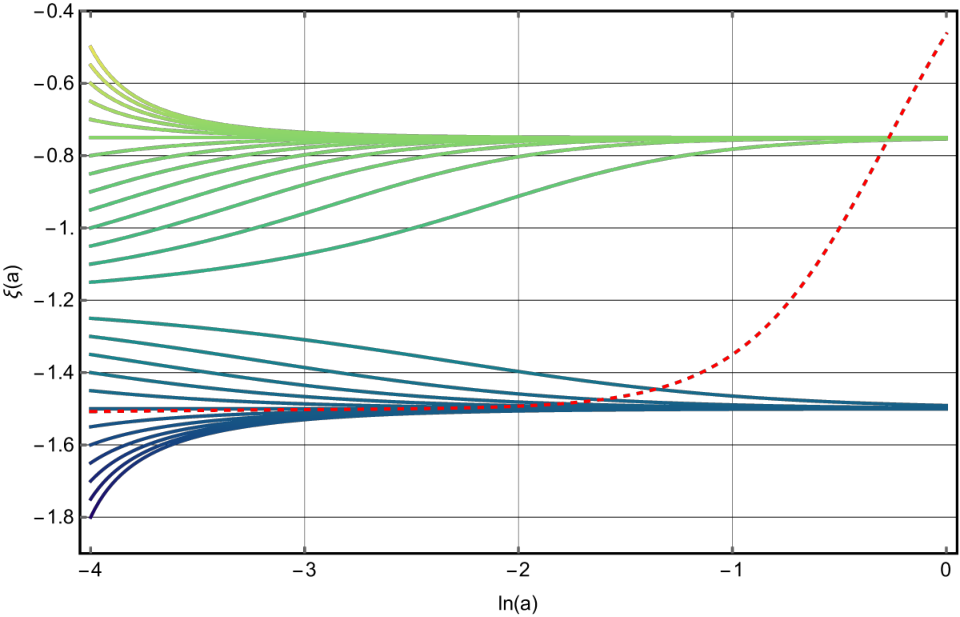
Through a stability analysis of the linearized dynamical system we find that the the critical point $\xi_{-}$ is a stable attractor only for $-4\leq\alpha\leq 0$. The critical point $\xi_{+}$ is a stable attractor for $\alpha\leq 0$, while the linear analysis alone cannot assess the stability of the point $\xi=-3/2$. These findings are supported by the numerical investigation shown in Fig. 2, so that the cosmic evolution will end up either at $\xi_{+}$ or $\xi_{-}$, depending on whether the initial $w_{\rm eff}$ is above or below the singularity at $w_{\rm eff}=-0.2$. The crucial point is that no trajectory can cross the $w_{\rm eff}=-0.2$ ridge; consequently, as anticipated on general grounds, the cosmic expansion cannot move from a decelerated phase around $w_{\rm eff}=0$ to an accelerated one around $w_{\rm eff}\approx-0.7$.

When matter is composed of dust plus a cosmological constant, we derive instead the following equation for $\xi,\Omega_{m}$,

$$\xi^{\prime\prime}=\frac{6(5\xi+6)^{4}\Omega_{m}+\xi(5\xi+6)^{2}\left(9(\alpha+16)+(\alpha+100)\xi^{2}+6(\alpha+40)\xi\right)+135\alpha\left(\xi^{\prime}\right)^{2}-27\alpha\left(5\xi^{2}+11\xi+6\right)\xi^{\prime}}{9\alpha(5\xi+6)}\;,$$

(26)

to be complemented by the conservation equation

$$\Omega_{m}^{\prime}=-(3+2\xi)\Omega_{m}\;.$$

(27)

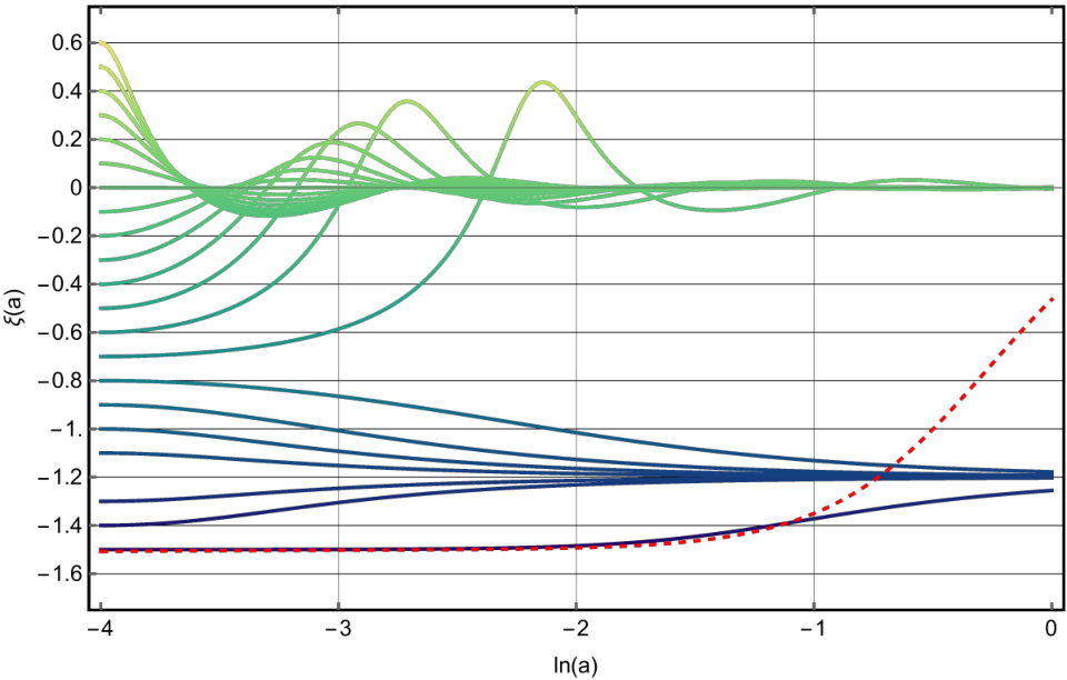
The phase space now is more complicated, in particular we found that now $\xi_{-}$ is always unstable and $\xi_{+}$ is a stable attractor for $\alpha<-16$. The critical point $\xi=-3/2$ is always unstable, while a new critical point $\xi=0$, i.e. a de Sitter state, appears which is a stable attractor when $-16\leq\alpha\leq 0$. However, the bottom line is the same, as can be immediately gleaned from Fig. 3, so the model is ruled out as a candidate for dark energy even when a cosmological constant is added, regardless of the value of $\alpha$.

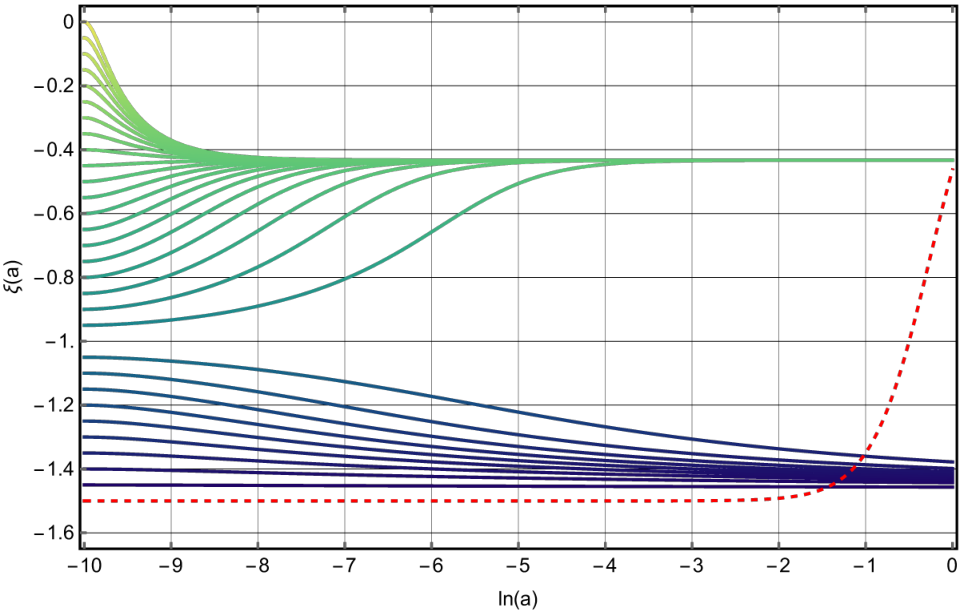
We also analysed numerically the case $L=R+\alpha R^{2}A$ and found a qualitatively very similar behavior (see Fig. 4), now with a divide at $\xi=-1$ as expected.

Here we discuss some ways to avoid the no-go theorem.

The anticurvature tensor, defined as the inverse of the Ricci tensor, allows the formulation of an alternative theory of gravity. Such a theory will have to be analysed to assess the existence of ghosts or other instabilities and derive the effects on perturbations such as the propagation of gravitational waves, the growth of perturbations, or the Newtonian limit. After deriving the general equations of motion for a generic Lagrangian function of the curvature and the anticurvature scalars, here we concerned ourselves about whether such a theory could be a viable candidate as a cosmological model. We have shown that a general no-go theorem prevents cosmic trajectories to join a decelerated phase to an accelerated one in any Lagrangian that contains a term with any positive or negative power of the anticurvature scalar, thereby ruling out a vast class of models. This no-go theorem is illustrated analytically and numerically in some particularly simple cases of models without new dimensional scales. We discuss possible ways out of the theorem, and in particular we point out some (more complicate) Lagrangians that avoid it. We leave to future work a systematic study of such models, in search of novel phenomenology.

We thank Tomi Koivisto, Ignacy Sawicki, and Oliver Piattella for useful comments on the draft. L.G. is grateful to the ITP-Heidelberg for the kind hospitality. His work was financed in part by the Coordenação de Aperfeiçoamento de Pessoal de Nível Superior - Brasil (CAPES) - Finance Code 001 and from the DAAD Co-financed Short-Term Research Grant Brazil, 2019 (57479964). L.A. acknowledges support from DAAD PPP Brasilien 57518956 (2020).

References

- Kaluza (2018) T. Kaluza, Preuss. Akad. Wiss. Berlin (Math. Phys.) 1921, 966; English translation: Int. J. Mod. Phys. D 27, 1870001 (2018), arXiv:1803.08616 [physics.hist-ph] .
- Klein (1926) O. Klein, Z. Phys. 37, 895 (1926).
- Dirac (1937) P. A. Dirac, Nature 139, 323 (1937).
- Dirac (1938) P. A. M. Dirac, Proceedings of the Royal Society of London Series A 165, 199 (1938).
- Eddington (1923) A. S. Eddington, The mathematical theory of relativity (1923).
- Schrödinger (1945) E. Schrödinger, Proceedings of the Royal Irish Academy. Section A: Mathematical and Physical Sciences 51, 163 (1945).
- Riess et al. (1998) A. G. Riess et al. (Supernova Search Team), Astron. J. 116, 1009 (1998), arXiv:astro-ph/9805201 .
- Perlmutter et al. (1999) S. Perlmutter et al. (Supernova Cosmology Project), Astrophys. J. 517, 565 (1999), arXiv:astro-ph/9812133 [astro-ph] .
- Weinberg (1989) S. Weinberg, Rev. Mod. Phys. 61, 1 (1989).
- Padilla (2015) A. Padilla, (2015), arXiv:1502.05296 [hep-th] .
- Bernal et al. (2016) J. L. Bernal, L. Verde, and A. G. Riess, JCAP 10, 019, arXiv:1607.05617 [astro-ph.CO] .
- Battye et al. (2015) R. A. Battye, T. Charnock, and A. Moss, Phys. Rev. D 91, 103508 (2015), arXiv:1409.2769 [astro-ph.CO] .
- Deser and Woodard (2007) S. Deser and R. P. Woodard, Phys. Rev. Lett. 99, 111301 (2007), arXiv:0706.2151 [astro-ph] .
- Woodard (2014) R. P. Woodard, Found. Phys. 44, 213 (2014), arXiv:1401.0254 [astro-ph.CO] .
- Deser and Woodard (2019) S. Deser and R. P. Woodard, (2019), arXiv:1902.08075 [gr-qc] .
- Park and Dodelson (2013) S. Park and S. Dodelson, Phys. Rev. D87, 024003 (2013), arXiv:1209.0836 [astro-ph.CO] .
- Dodelson and Park (2014) S. Dodelson and S. Park, Phys. Rev. D90, 043535 (2014), [Erratum: Phys. Rev.D98,no.2,029904(2018)], arXiv:1310.4329 [astro-ph.CO] .
- Nersisyan et al. (2017) H. Nersisyan, A. F. Cid, and L. Amendola, JCAP 1704 (04), 046, arXiv:1701.00434 [astro-ph.CO] .
- Amendola et al. (2019) L. Amendola, Y. Dirian, H. Nersisyan, and S. Park, JCAP 1903 (03), 045, arXiv:1901.07832 [astro-ph.CO] .
- Carroll et al. (2005) S. M. Carroll, A. De Felice, V. Duvvuri, D. A. Easson, M. Trodden, and M. S. Turner, Phys. Rev. D 71, 063513 (2005), arXiv:astro-ph/0410031 .
- Allemandi et al. (2004) G. Allemandi, A. Borowiec, and M. Francaviglia, Phys. Rev. D 70, 103503 (2004), arXiv:hep-th/0407090 .
- Li et al. (2007) B. Li, J. D. Barrow, and D. F. Mota, Phys. Rev. D 76, 104047 (2007), arXiv:0707.2664 [gr-qc] .
- Capozziello and Laurentis (2011) S. Capozziello and M. D. Laurentis, Physics Reports 509, 167 (2011).
- Deser and Gibbons (1998) S. Deser and G. W. Gibbons, Classical and Quantum Gravity 15, L35 (1998), arXiv:hep-th/9803049 [hep-th] .
- Stelle (1978) K. S. Stelle, General Relativity and Gravitation 9, 353 (1978).
- Chiba (2005) T. Chiba, JCAP 2005 (3), 008, arXiv:gr-qc/0502070 [astro-ph] .
- Abbott et al. (2019) T. Abbott et al. (DES), Astrophys. J. Lett. 872, L30 (2019), arXiv:1811.02374 [astro-ph.CO] .
- Scolnic et al. (2018) D. Scolnic et al., Astrophys. J. 859, 101 (2018), arXiv:1710.00845 [astro-ph.CO] .
- Aghanim et al. (2018) N. Aghanim et al. (Planck), (2018), arXiv:1807.06209 [astro-ph.CO] .
- Ade et al. (2016) P. A. R. Ade et al. (Planck), Astron. Astrophys. 594, A13 (2016), arXiv:1502.01589 [astro-ph.CO] .
- Migkas et al. (2020) K. Migkas, G. Schellenberger, T. Reiprich, F. Pacaud, M. Ramos-Ceja, and L. Lovisari, Astron. Astrophys. 636, A15 (2020), arXiv:2004.03305 [astro-ph.CO] .