跳到论文正文
W Papers独立论文阅读器 arXiv:2006.04117 论文正文 计算阅读时间 · 0%
引用这篇论文根据当前论文元数据生成,正式投稿前建议核对。


License: arXiv.org perpetual non-exclusive license
arXiv:2006.04117v1 [cs.LG] 07 Jun 2020

Sharp Thresholds of the Information Cascade Fragility Under a Mismatched Model

Wasim Huleihel Thanks: W. Huleihel and O. Shayevitz are with the Department of Electrical Engineering-Systems at Tel-Aviv university, Tel-Aviv 6997801, Israel (e-mail: {wasimh,ofersha@mail,eng}.tau.ac.il). This research was supported by the European Research Council (ERC) under grant agreement 639573.    Ofer  Shayevitz11footnotemark: 1
Abstract

We analyze a sequential decision making model in which decision makers (or, players) take their decisions based on their own private information as well as the actions of previous decision makers. Such decision making processes often lead to what is known as the information cascade or herding phenomenon. Specifically, a cascade develops when it seems rational for some players to abandon their own private information and imitate the actions of earlier players. The risk, however, is that if the initial decisions were wrong, then the whole cascade will be wrong. Nonetheless, information cascade are known to be fragile: there exists a sequence of revealing probabilities {pℓ}ℓ≥1\{p_{\ell}\}_{\ell\geq 1}, such that if with probability pℓp_{\ell} player ℓ\ell ignores the decisions of previous players, and rely on his private information only, then wrong cascades can be avoided. Previous related papers which study the fragility of information cascades always assume that the revealing probabilities are known to all players perfectly, which might be unrealistic in practice. Accordingly, in this paper we study a mismatch model where players believe that the revealing probabilities are {qℓ}ℓ∈ℕ\{q_{\ell}\}_{\ell\in\mathbb{N}} when they truly are {pℓ}ℓ∈ℕ\{p_{\ell}\}_{\ell\in\mathbb{N}}, and study the effect of this mismatch on information cascades. We consider both adversarial and probabilistic sequential decision making models, and derive closed-form expressions for the optimal learning rates at which the error probability associated with a certain decision maker goes to zero. We prove several novel phase transitions in the behaviour of the asymptotic learning rate.

1 Introduction

There are myriad economic and social scenarios where our decisions are influenced by the actions of others. For example, voters are inclined to vote in favor of what opinion polls predicts will win. Academic researchers choose to work on topics that are of broad and current interest. Fertility decisions, e.g., how many children to have, are known to be influenced by what other people in the same geographical location are doing. Opinions we hold, products we buy, and technologies we use, etc., are all potentially affected by our surroundings. The above is a non-exhaustive list of scenarios where our rational behaviour guides us to follow the actions of others despite the fact that these may contradict our own information. This is exactly the situation where information cascades [5, 7] develop.

To illustrate the way information cascades evolve we consider the following simple and classical herding experiment, proposed and studied in [3, 2] (see also [9, Ch. 16]). In this experiment, we place an urn that contains three marbles in front of a bunch of players. The urn contains either one red marble and two blue marbles (majority blue), or, two red marbles and one blue marble (majority red). Players do not know whether the urn is majority blue or red, while both urns are equally likely to be chosen. In a successive manner, each player randomly draws a single marble from the urn, memorizes its color, and returns it to the urn, while not showing it to the other players. Then, each player in his turn publicly announce his guess for the urn majority color. The players guesses are based on both their own private draws as well as the actions/announcements of previous players.

Next, we explain how the above experiment evolves. It is clear that the first two players will announce their private signals as their guesses. Indeed, the first player gets to see his own draw only, and thus his best guess for the urn majority color is the color he draw. The second player is aware of that, and thus, together with his own draw he gets to see two independent draws from the urn. Accordingly, if the colors agree, then the player announces this color; otherwise, there is a tie, and in such a case let us assume that the player follows his own draw. Therefore, it is clear again that the second player announces the color of the marble he draw. Continuing, the third player now see three independent draws from the urn and consequently his best decision is the majority color among these draws.

The most important observation here is that the rational guess of any subsequent player may not reflect its own private information. For example, if the first two announced colors were blue, then the third player guess is blue irrespectively of the color of the marble he picked. Evidently, due to the fact that his guess will not reveal any information about the urn to any subsequent player, every subsequent player will guess the urn to be majority blue. This is where an information cascade developed: while no one is under the impression that every player draw a blue marble, since the first two guesses were blue, future rational guesses must be blue as well. To wit, an information cascade is a sequence of decisions where it is optimal for players to ignore their own private information and imitate the decisions of players ahead of them. The problem with information cascade is that they can be wrong! Indeed, if for instance in the above example the urn is majority red, then everyone wrongly announced blue as their guesses. In fact, in the above experiment, it can be shown that with probability 1/51/5, a wrong cascade develops, in which case, most players will guess the urn majority color wrongly.

The experiment above illustrates that information cascades can be wrong because they rely on very little actual information–the actions of the first few players can determine the actions of all future players. Nonetheless, this hints that information cascades can also be fundamentally very fragile. Indeed, suppose that in the above experiment two consecutive players ℓ\ell and ℓ+1\ell+1 draw red marbles, and they cheat (or, act irrationally) by announcing their marbles despite the fact that a majority-blue cascade was already developed (say, the first two players announced blue). Then, it is clear that the wrong cascade can be broken: player ℓ+2\ell+2 sees four informative draws (two blues and two reds), and he will announce his own private signal as his guess. The conclusion is that infusion of new information can overturn/brake wrong information cascades even after they have persisted for a long time.

Motivated by the above observation, we consider a simple sequential decision making model in which not all players are rational, but rather certain players act irrationally, by revealing their own private signal and discarding the actions of previous players. More specifically, we focus on a recent model proposed by [17], where it is assumed that the ℓ\ellth player is irrational/revealer with some probability pℓp_{\ell}, and is rational/Bayesian with complementary probability. While players do not know whether other players before them were rational or not, it is assumed in [17] nonetheless that players know the revealing probabilities {pℓ}ℓ∈ℕ\{p_{\ell}\}_{\ell\in\mathbb{N}}. As mentioned in [17], this model is prompted by both empirical laboratory experiments [2, 14, 19], as well as several theoretical reasons [6]. One of the intriguing questions here, is whether wrong information cascades are broken in the above model? Or, stated differently, do people eventually learn the correct action? As was shown in [17], the answer to this question is positive. Namely, it can be shown that there exists a sequence of revealing probabilities {pℓ}ℓ∈ℕ\{p_{\ell}\}_{\ell\in\mathbb{N}} such that learning occurs. In particular, the optimal policy minimizing the probability of error is for the ℓ\ellth player to reveal its private signal with probability pℓ=c/ℓp_{\ell}=c/\ell, which in turn implies a learning rate of c′/ℓc^{\prime}/\ell, where cc and c′c^{\prime} are explicit constants. While these results are neat, as mentioned in [17] they rely heavily on the assumption that players are fully coordinated, i.e., they know the revealing probabilities exactly, which might be unrealistic in practice. This sets precisely the main goal of our paper: we aim to understand how this coordination affects information cascades. To this end, we introduce a mismatch model where players believe that the revealing probabilities are {qℓ}ℓ∈ℕ\{q_{\ell}\}_{\ell\in\mathbb{N}} when they truly are {pℓ}ℓ∈ℕ\{p_{\ell}\}_{\ell\in\mathbb{N}}. We are interested in understanding whether asymptotic learning occur in this case? and if so, under what conditions and at what learning rate? In particular, what is the cost of this mismatch?

The above mismatch model might be relevant in many real-world applications, such as, rumor spreading over social networks, online movie rating, etc., where it is well-documented that human behavior is sometimes irrational (e.g., [15]). Furthermore, it is well-known in the social learning literature that a fully rational model often places unreasonable computational demands on Bayesian players (e.g., [16]), hence understanding the impact of simpler more efficient strategies is desirable. As we explain in the paper, this situation can be partially captured by our model, since our mismatch framework allow for a family of sub-optimal strategies parameterized by the mismatch sequence {qℓ}ℓ∈ℕ\{q_{\ell}\}_{\ell\in\mathbb{N}}.

Main Contributions. The main contributions of this paper are as follows. We start by formulating a general adversarial/worst-case model where the placement of irrational players is arbitrary, and not being governed by any probabilistic/statistical rule. We show that this kind of model is in fact too stringent leading to trivial results. Combined with [17], this fact motivates us to study the more flexible probabilistic model described above. For this model we characterize the asymptotic learning rate exactly, which turns out to exhibit several novel interesting phase transitions. Specifically, we first show that for either too “optimistic” or “pessimistic” assumptions, i.e., qt=o⁡(pt)q_{t}=o(p_{t}) or qt=ω⁡(pt)q_{t}=\omega(p_{t}), asymptotic learning does not occur, namely, the error probability is high, and the total number of wrong decisions is significant. We then consider the case where qt=Θ⁡(pt)q_{t}=\Theta(p_{t}), and show that asymptotic learning occurs, but at a reduced rate which loosely speaking depends on the ratio between the ℓ1\ell_{1}-norms of the matched and mismatched revealing probabilities. This is true, as long as the magnitude of this ratio is moderate laying between two thresholds, otherwise, asymptotic learning does not occur!

Related work. Sequential decision making has been studied in various areas including politics, economics and computer science. In particular, the case where all players are Bayesian (i.e., pℓ=0,∀ℓp_{\ell}=0,\forall\ell) was considered in [9, 5, 7]. Notably, [7] gives many interesting real-world examples from diverse fields, where information cascades develop and are fragile. Similarly to [17], our paper provides a more detailed theoretical study of the fragility phenomenon. In practice, however, it is well documented, that human behavior deviates from rationality, and rather irrational decisions are made often, see, e.g., [15, 14] and [19]. Indeed, several laboratory experiments in [3] illustrate that many individuals act irrationally, by ignoring the actions of other individuals and relying mainly on their own private information. Our model captures this empirically observed behavioral phenomenon.

In [6], a model which combines both rational and partially irrational (who put more weight on their private signal) types of individuals, as in our model, was studied. It is assumed, however, that players know which of the previous players were revealers. Using simulations it was suggested that learning is achievable only when completely irrational individuals exist, and that their fraction should vanish. These observations were rigorously proved in [17], showing that the optimal number of revealers is logarithmic in the size of the group. Our results show that in many cases learning is possible even if there is a mismatch. Recently, [8] also considered a model with irrational players, but assume that each agent knows which agents were revealers. While they show that asymptotic learning occurs, the optimal learning rate was not characterized, which is another contribution of our paper when there is a mismatch. Sequential decision models with unbounded private signals (e.g., Gaussian) were studied in [18, 12]. We also mention the study of sequential decision making models over social random graphs, e.g., [1, 4]. Finally, we mention another somewhat related literature which studies the situation where agents take repeated decisions (rather than just a single decision) based on their own private information and the actions of others, e.g., [13], and one is interested in understanding whether all decision makers learn the correct state eventually, and if so at what speed.

2 Problem Setup

In this section, we present our model and formulate the problem of interest. To convey neatly the main ideas of this paper, we focus on a simple setting of the information cascade model. Nonetheless, several generalizations listed at the end of this paper, can be derived using the same techniques used in this paper. Let θ∈{1,2}\theta\in\{1,2\} denote the state of the world, chosen uniformly at random. At times t=1,2,3,…t=1,2,3,\ldots, players one by one try to guess θ\theta, relying on their own private signals, as well as the global actions (guesses) of players who played before them.

We next describe the way private signals are formed. There is an urn that contains two types of marbles: Type–I marbles are blue, and Type–II are red. There are two hypotheses depending on the value of θ\theta. Specifically, given θ\theta, there are α\alpha marbles of type θ\theta in the urn, and β\beta marbles of the other type, where we assume that α>β>0\alpha>\beta>0. We conduct the following experiment: each player draws a single marble from the urn and replace it. The color he draw is his private signal. Thus, the private signals denoted by X1,X2,…X_{1},X_{2},\ldots are i.i.d., and:

ℙ1​(Xt=1)=αα+β;ℙ1​(Xt=2)=βα+β,\displaystyle\mathbb{P}_{1}(X_{t}=1)=\frac{\alpha}{\alpha+\beta};\quad\quad\mathbb{P}_{1}(X_{t}=2)=\frac{\beta}{\alpha+\beta},
ℙ2​(Xt=1)=βα+β;ℙ2​(Xt=2)=αα+β,\displaystyle\mathbb{P}_{2}(X_{t}=1)=\frac{\beta}{\alpha+\beta};\quad\quad\mathbb{P}_{2}(X_{t}=2)=\frac{\alpha}{\alpha+\beta},

where ℙi(⋅)≜ℙ(⋅|θ=i)\mathbb{P}_{i}(\cdot)\triangleq\mathbb{P}(\cdot|\theta=i), and t∈ℕt\in\mathbb{N}. It is clear that the ratio α/β\alpha/\beta, rather than the actual values of α\alpha and β\beta, is important. We denote this ratio by γ≜α/β\gamma\triangleq\alpha/\beta. Note that an alternative equivalent description of the above setting is that at each time tt, the ttth player private signal is Xt=θX_{t}=\theta with some probability, and Xt=3−θX_{t}=3-\theta, with the complementary probability. With θ\theta being latent, the players goal is to guess the type of the marbles in the urn correctly. We denote by ZtZ_{t} the guess of the ttth player. As mentioned in the introduction, if all players act rationally by announcing their majority decision, then with positive probability (wrong) information cascade will occur. Accordingly, to break this wrong information cascade, we assume that each player, can operate in either one of the following two modes:

  • •

    A revealer/irrational player, whose guess is simply its private signal, i.e., Zt=XtZ_{t}=X_{t}.

  • •

    A Bayesian/rational player, whose guess is its best estimate given his private signal, previous guesses by other players, and any additional auxiliary information.

Given the two modes above, it is left to specify the way players are “chosen” to be in either one of the above modes, which is the last aspect of our model. We start with a general adversarial/worst-case machinery, which turns out to be too stringent, and as a consequence leads to trivial results. Nonetheless, this model will motivate our second probabilistic setting, which is the focus of this paper.

In the adversarial setting, we assume that out of a total of 𝖭∈ℕ\mathsf{N}\in\mathbb{N} players 𝖵𝖭∈ℕ\mathsf{V_{N}}\in\mathbb{N} are irrational, and are chosen in an arbitrary manner. We let Π𝖭\Pi_{\mathsf{N}} be the set of these irrational players. Players do not know whether previous players were rational or not, but they do have the value of 𝖵𝖭\mathsf{V_{N}} in advance. We define the probability of incorrect decision of the ttth player, assuming that he is rational, as follows,

𝖯𝖺𝖽𝗏,t​(𝖵𝖭)\displaystyle\mathsf{P}_{\mathsf{adv},t}(\mathsf{V_{N}}) ≜infθ^t∈Θ^supΠ𝖭⊂[𝖭]:|Π𝖭|=𝖵𝖭𝖯e,t(θ^t,Π𝖭),\displaystyle\triangleq\inf_{\hat{\theta}_{t}\in\hat{\Theta}}\sup_{\Pi_{\mathsf{N}}\subset[\mathsf{N}]:\;|\Pi_{\mathsf{N}}|=\mathsf{V_{N}}}\mathsf{P}_{e,t}(\hat{\theta}_{t},\Pi_{\mathsf{N}}), (1)

and

𝖯e,t(θ^t,Π𝖭)≜ℙ[θ^t(Z1t−1,Xt)≠θ|𝖱𝖾𝗏𝖭=Π𝖭],\displaystyle\mathsf{P}_{e,t}(\hat{\theta}_{t},\Pi_{\mathsf{N}})\triangleq\mathbb{P}\left[\left.\hat{\theta}_{t}(Z_{1}^{t-1},X_{t})\neq\theta\right|\mathsf{Rev}_{\mathsf{N}}=\Pi_{\mathsf{N}}\right], (2)

where Z1t−1Z_{1}^{t-1} is a shorthand notation for the sequence (Z1,Z2,…,Zt−1)(Z_{1},Z_{2},\ldots,Z_{t-1}), 𝖱𝖾𝗏𝖭\mathsf{Rev}_{\mathsf{N}} designates the set of revealers, the maximum is taken over all possible sets of revealers of size 𝖵𝖭\mathsf{V_{N}}, and the minimum is over the set of all possible estimators Θ^\hat{\Theta}, which are the Boolean maps {1,2}t→{1,2}\{1,2\}^{t}\to\{1,2\}. To wit, we look at the worst-case error probability over all possible choices of 𝖵𝖭\mathsf{V_{N}} irrational players out of 𝖭\mathsf{N} players. An alternative objective is to minimize the expected total number of errors, that is,

𝖳𝖤(𝖵𝖭)≜infθ^∈Θ^supΠ𝖭⊂[𝖭]:|Π𝖭|=𝖵𝖭∑t=1𝖭𝖯e,t(θ^t,Π𝖭).\displaystyle\mathsf{TE}(\mathsf{V_{N}})\triangleq\inf_{\hat{\theta}\in\hat{\Theta}}\sup_{\Pi_{\mathsf{N}}\subset[\mathsf{N}]:\;|\Pi_{\mathsf{N}}|=\mathsf{V_{N}}}\sum_{t=1}^{\mathsf{N}}\mathsf{P}_{e,t}(\hat{\theta}_{t},\Pi_{\mathsf{N}}). (3)

For both objectives, it is a-priori unclear what is the optimal strategy θ^t\hat{\theta}_{t}. One option, which is simple and widely used in practice, is to assume that each rational player guesses the value of θ\theta using the majority decision, denoted by 𝖬𝖺𝗃⁡(Z1t−1,Xt)\mathsf{Maj}(Z_{1}^{t-1},X_{t}). A more complicated approach is to minimize over the Boolean functions used by the rational players, i.e., to solve a minimax problem. We would like to find the asymptotic behaviour of 𝖯𝖺𝖽𝗏,t​(𝖵𝖭)\mathsf{P}_{\mathsf{adv},t}(\mathsf{V_{N}}) and 𝖳𝖤⁡(𝖵𝖭)\mathsf{TE}(\mathsf{V_{N}}), as a function of 𝖵𝖭\mathsf{V_{N}} and tt. In particular, it is interesting to understand the structure of the worst-case choice of the set of the irrational players Π𝖭\Pi_{\mathsf{N}}. It turns out that the above model/objective, however, is too stringent. Specifically, we show in Section 4.4 that the error probability in (1) associated with any estimator is lower bounded by a constant, and accordingly, the total number of errors in (3) is proportional to the number of players 𝖭\mathsf{N}. This implies that there are no guessing strategies that are robust against an arbitrary adversarial revealers assignment. Therefore, a more flexible model is needed.

To this end, we consider the probabilistic setting introduced in [17]. Here, we assume that the ttth player is irrational with probability ptp_{t}, independently of the other players. Accordingly, this means that if player tt is irrational, then Zt=XtZ_{t}=X_{t}, while if he is rational, then Zt=θ^t​(Z1,…,Zt−1,Xt)Z_{t}=\hat{\theta}_{t}(Z_{1},\ldots,Z_{t-1},X_{t}), where θ^\hat{\theta} is a certain estimator for θ\theta. The main important ingredient of our model is that we assume that players are completely oblivious to whether previous players were revealers or not. To wit, contrary to previous related works (e.g., [6, 8, 17]), we assume that revealers neither know the exact positioning of revealers, nor the underlying probabilistic law of their placements. Instead, players assume that other players can be revealers with probabilities 𝒬≡{qt}t=1∞{\cal Q}\equiv\{q_{t}\}_{t=1}^{\infty}, which might be different than the actual underlying probabilities 𝒫≡{pt}t=1∞{\cal P}\equiv\{p_{t}\}_{t=1}^{\infty}. In that case, we say that there is a mismatch. Thus, estimators θ^t\hat{\theta}_{t} might be in fact a function of 𝒬{\cal Q} as well. The matched case case where 𝒫=𝒬{\cal P}={\cal Q} was considered in [17].

Whenever a player is rational we assume that he tries to do his best in guessing θ\theta under the knowledge of 𝒬{\cal Q}. Namely, a rational player employs the (mismatched) maximum a posteriori probability (MAP) estimator, which is simply the MAP estimator, but with 𝒫{\cal P} replaced by 𝒬{\cal Q}. Specifically, for i∈{1,2}i\in\{1,2\} and t≥1t\geq 1, define the distributions:

Wit​(z1t)\displaystyle W_{i}^{t}(z_{1}^{t}) ≜ℙi​(Z1t=z1t),\displaystyle\triangleq\mathbb{P}_{i}\left(Z_{1}^{t}=z_{1}^{t}\right), (4)
Hit​(z1t−1,xt)\displaystyle H_{i}^{t}(z_{1}^{t-1},x_{t}) ≜ℙi​(Z1t−1=z1t−1,Xt=xt),\displaystyle\triangleq\mathbb{P}_{i}\left(Z_{1}^{t-1}=z_{1}^{t-1},X_{t}=x_{t}\right), (5)

and the corresponding likelihood r.v.s by

𝖫it\displaystyle\mathsf{L}_{i}^{t} ≜Wit​(Z1t),\displaystyle\triangleq W_{i}^{t}(Z_{1}^{t}), (6)
𝖣it\displaystyle\mathsf{D}_{i}^{t} ≜Hit​(Z1t−1,Xt),\displaystyle\triangleq H_{i}^{t}(Z_{1}^{t-1},X_{t}), (7)

with 𝖫i0=𝖣i0=1\mathsf{L}_{i}^{0}=\mathsf{D}_{i}^{0}=1, for i∈{1,2}i\in\{1,2\}. Note that player tt can compute the likelihoods 𝖣it\mathsf{D}_{i}^{t}, for i=1,2i=1,2. The likelihoods 𝖫i0=𝖣i0=1\mathsf{L}_{i}^{0}=\mathsf{D}_{i}^{0}=1, for i∈{1,2}i\in\{1,2\}, can be computed by a “genie” who observes the decisions of the first tt players. The above probabilities and likelihoods are certain quite complicated functions of 𝒫{\cal P}. We let W^it\hat{W}_{i}^{t} and H^it\hat{H}_{i}^{t} be the corresponding probabilities with 𝒫{\cal P} replaced by 𝒬{\cal Q}. We also define 𝖫^it\hat{\mathsf{L}}_{i}^{t} and 𝖣^it\hat{\mathsf{D}}_{i}^{t} in the same way, but with WitW_{i}^{t} and HitH_{i}^{t} replaced by W^it\hat{W}_{i}^{t} and H^it\hat{H}_{i}^{t}, respectively. With these definitions, the mismatched MAP estimate, denoted by Zt=𝖬𝖠𝖯𝒬​(Z1t−1,Xt)Z_{t}=\mathsf{MAP}_{{\cal Q}}(Z_{1}^{t-1},X_{t}), is:

𝖬𝖠𝖯𝒬​(Z1t−1,Xt)≜{1,𝖣^1t>𝖣^2t,2,𝖣^1t<𝖣^2t,Xt,𝖣^1t=𝖣^2t.\displaystyle\mathsf{MAP}_{{\cal Q}}(Z_{1}^{t-1},X_{t})\triangleq\begin{cases}1,\ &\hat{\mathsf{D}}_{1}^{t}>\hat{\mathsf{D}}_{2}^{t},\\ 2,\ &\hat{\mathsf{D}}_{1}^{t}<\hat{\mathsf{D}}_{2}^{t},\\ X_{t},\ &\hat{\mathsf{D}}_{1}^{t}=\hat{\mathsf{D}}_{2}^{t}.\end{cases} (8)

Thus, the mismatch aspect in our setup lies in the fact that the ttth player estimator function depends on 𝒬{\cal Q}, and more importantly, independent of 𝒫{\cal P}. We mention here that the above estimator in fact provides a family of possible estimators indexed by 𝒬{\cal Q}. For instance, 𝒬≡1{\cal Q}\equiv 1 corresponds to majority decisions, for which rational players guesses are simply the majority color of their own private and previously announced signals.

Players try to guess the urn majority color. We define the probability of incorrect guess by the ttth player, as follows,

𝖯e,t​(𝒫,𝒬)≜ℙ⁡(Zt≠θ).\displaystyle\mathsf{P}_{e,t}({\cal P},{\cal Q})\triangleq\mathbb{P}\left(Z_{t}\neq\theta\right). (9)

Our goal is to understand the asymptotic learning rate at which the above error probability decays to zero as a function of tt (i.e., learning occurs). To motivate and define our objective precisely, we recall the following recent result which deals with the matched case where 𝒫=𝒬{\cal P}={\cal Q}.

Theorem 1.

[17, Theorem 1.1] Let

κ⁡(γ)≜[1+γ−1log⁡γ​(log⁡γ−1log⁡γ−1)]−1.\displaystyle\kappa(\gamma)\triangleq\left[1+\frac{\gamma-1}{\log\gamma}\left(\log\frac{\gamma-1}{\log\gamma}-1\right)\right]^{-1}. (10)

Then,

inf𝒫lim supt→∞t⋅𝖯e,t​(𝒫,𝒫)=κ⁡(γ).\displaystyle\inf_{{\cal P}}\limsup_{t\to\infty}t\cdot\mathsf{P}_{e,t}({\cal P},{\cal P})=\kappa(\gamma). (11)

Moreover, one can be arbitrarily close to the optimum by taking,

pt⋆=(1+ε)⋅(1+γ)​κ​(γ)t∧1,\displaystyle p_{t}^{\star}=(1+\varepsilon)\cdot\frac{(1+\gamma)\kappa(\gamma)}{t}\wedge 1, (12)

for t≥1t\geq 1 and arbitrary ϵ>0\epsilon>0.

Theorem 1 states that the optimal learning rate is Θ⁡(1/t)\Theta(1/t), and furthermore provides the exact leading constant in (10). To achieve this optimal learning rate, the revealing probabilities should also decay as Θ⁡(1/t)\Theta(1/t). The intuitive reasoning behind these findings can be found in [17, Sec. 1.2]. With this result in mind, in the mismatch case where 𝒬≠𝒫{\cal Q}\neq{\cal P}, we focus on the following scenario. We assume that 𝒫=𝒫⋆{\cal P}={\cal P}^{\star}, where 𝒫⋆{\cal P}^{\star} is defined in (12). In other words, the underlying revealing probabilities sequence is the optimal one, while players assume a (possibly) different sequence of revealing probabilities 𝒬{\cal Q}. For simplicity of demonstration, we opted to focus on this special case since we found it to be the most natural one. Nonetheless, our techniques apply also for the more general case where 𝒫≠𝒫⋆{\cal P}\neq{\cal P}^{\star}, and at the end of the following section we cover with this case too. It is then interesting to understand whether such a mismatch has any effect whatsoever on the achieved learning rate. In particular, does asymptotic learning always occur? or, perhaps there is a sequence of revealing probabilities 𝒬{\cal Q} for which learning is impossible. To answer these questions, we aim to characterize the polynomial learning rate, defined as follows,

𝖤(𝒫,𝒬)≜lim inft→∞−log⁡𝖯e,t​(𝒫,𝒬)log⁡t.\displaystyle\mathsf{E}({\cal P},{\cal Q})\triangleq\liminf_{t\to\infty}-\frac{\log\mathsf{P}_{e,t}({\cal P},{\cal Q})}{\log t}. (13)

To lower bound 𝖤⁡(𝒫,𝒬)\mathsf{E}({\cal P},{\cal Q}) we upper bound the error probability 𝖯e,t​(𝒫,𝒬)\mathsf{P}_{e,t}({\cal P},{\cal Q}), which in turn can be used to upper bound the expected total number of errors:

𝖳𝖤t≜𝔼[∑ℓ=1t𝟙[Zℓ≠θ]].\displaystyle\mathsf{TE}_{t}\triangleq\mathbb{E}\left[\sum_{\ell=1}^{t}\mathds{1}\left[Z_{\ell}\neq\theta\right]\right]. (14)

Accordingly, a positive polynomial decaying learning rate implies that 𝖳𝖤t=o⁡(t)\mathsf{TE}_{t}=o(t), i.e., the number of errors is negligible compared to the total number of players participated thus far. It is clear that Theorem 1 implies that 𝖤⁡(𝒫⋆,𝒫⋆)=1\mathsf{E}({\cal P}^{\star},{\cal P}^{\star})=1, and in fact that 0≤𝖤⁡(𝒫⋆,𝒬)≤10\leq\mathsf{E}({\cal P}^{\star},{\cal Q})\leq 1, for any 𝒬{\cal Q}. We would like to understand when it is possible or impossible to obtain a positive polynomial decaying learning rate, i.e., when 𝖤⁡(𝒫⋆,𝒬)>0\mathsf{E}({\cal P}^{\star},{\cal Q})>0. Note that an interesting question is to characterize the specific constant in front of the polynomial decaying term by evaluating limt→∞t𝖤⁡(𝒫,𝒬)⋅𝖯e,t​(𝒫,𝒬)\lim_{t\to\infty}t^{\mathsf{E}({\cal P},{\cal Q})}\cdot\mathsf{P}_{e,t}({\cal P},{\cal Q}), which we leave as an open question for future research. Finally, note that Theorem 1 gives a simple lower bound on 𝖯e,t​(𝒫⋆,𝒬)\mathsf{P}_{e,t}({\cal P}^{\star},{\cal Q}) because of the trivial inequality 𝖯e,t​(𝒫⋆,𝒬)≥𝖯e,t​(𝒫⋆,𝒫⋆)\mathsf{P}_{e,t}({\cal P}^{\star},{\cal Q})\geq\mathsf{P}_{e,t}({\cal P}^{\star},{\cal P}^{\star}). Indeed, for each player seeking to minimize the error probability, its best action is to output the (matched) MAP decision. It is interesting to note that this observation also follows from

𝖯e,t​(𝒫⋆,𝒬)≥βα+β⋅pt⋆=κ⁡(γ)t,\displaystyle\mathsf{P}_{e,t}({\cal P}^{\star},{\cal Q})\geq\frac{\beta}{\alpha+\beta}\cdot p_{t}^{\star}=\frac{\kappa(\gamma)}{t}, (15)

for tt large enough, and the first inequality follows because βα+β​pt⋆\frac{\beta}{\alpha+\beta}p_{t}^{\star} is the error probability when player tt acts on its private information only (i.e., revealer), while we ignore the error resulted when player tt is rational. This lower bound, however, is not tight as we show in the following section. For the rest of this paper, we let 𝒫t≜(p1,p2,…,pt){\cal P}_{t}\triangleq(p_{1},p_{2},\ldots,p_{t}), and ‖⋅‖\left\|\cdot\right\| denotes the ℓ1\ell_{1}-norm.

3 Main Results

In this section, we study the probabilistic setting described in the previous section. According to Theorem 1, to achieve the optimal learning rate the revealing probabilities should decay as Θ⁡(t−1)\Theta(t^{-1}). Note that it is clear that the revealing probabilities cannot decay to zero too quickly. Indeed, if for example ‖𝒫‖<∞\left\|{\cal P}\right\|<\infty, then by the Borel-Cantelli lemma there will be only a finite number of revealers almost surely, which is equivalent to the situation where no revealers exist. This in turn implies a non-vanishing error probability. The situation is somewhat similar when the revealing probabilities decay to zero too slowly. Intuitively, in this case, it can be shown that the error probability is dominated by the probability that the ttth player is a revealer and announce a wrong decision, namely, βα+β​pt\frac{\beta}{\alpha+\beta}p_{t}. Therefore, if for example pt=Θ⁡(t−c)p_{t}=\Theta(t^{-c}), for some c∈(0,1)c\in(0,1), then 𝖤⁡(𝒫,𝒫)=c<𝖤⁡(𝒫⋆,𝒫⋆)\mathsf{E}({\cal P},{\cal P})=c<\mathsf{E}({\cal P}^{\star},{\cal P}^{\star}).

The optimal scaling of the revealing probabilities suggests that with high probability there should be ‖𝒫t‖∼log⁡t\left\|{\cal P}_{t}\right\|\sim\log t revealers, as t→∞t\to\infty. Accordingly, in terms of mismatch, it makes sense that “wise” players will assume that the revealing probabilities decay at the same order, but perhaps with a different constant in front, e.g., qt=ρ⋅ptq_{t}=\rho\cdot p_{t}, and ρ≠1\rho\neq 1. Nonetheless, as mentioned above, rather than modeling the imperfect knowledge of players about the revealing probabilities, our mismatched MAP can also model the situation where players intentionally employ sub-optimal strategies (e.g., in order to reduce computational complexity), such as when 𝒬≡1{\cal Q}\equiv 1, which results in majority decisions. While it is clear from the above that in the matched case it is strictly worse to assume that the revealing probabilities 𝒫{\cal P} decay to zero too quickly/slowly, it is a-priori unclear if this is true for 𝒬{\cal Q} as well. The following result shows that if the assumed revealing probabilities 𝒬{\cal Q} are either too small or too large, then asymptotic learning does not occur at all! In particular, 𝖤⁡(𝒫⋆,𝒬)=0\mathsf{E}({\cal P}^{\star},{\cal Q})=0. We have the following result.

Theorem 2 (Too quick/slow).

For any sequence of mismatched revealing probabilities 𝒬{\cal Q} such that,

lim inft→∞‖𝒬t‖log⁡t=0orlim supt→∞‖𝒬t‖log⁡t=∞,\displaystyle\liminf_{t\to\infty}\frac{\left\|{\cal Q}_{t}\right\|}{\log t}=0\quad\mathrm{or}\quad\limsup_{t\to\infty}\frac{\left\|{\cal Q}_{t}\right\|}{\log t}=\infty, (16)

we have 𝖤⁡(𝒫⋆,𝒬)=0\mathsf{E}({\cal P}^{\star},{\cal Q})=0.

Theorem 2 implies, for example, that if qt=o⁡(t−1)q_{t}=o(t^{-1}) or qt=ω⁡(t−1)q_{t}=\omega(t^{-1}), then the error probability cannot decay to zero polynomially fast. In fact, our proof gives a general lower bound on the probability of error which implies for instance that when ‖𝒬‖<∞\left\|{\cal Q}\right\|<\infty, then the probability of error is lower bounded by a constant. Indeed, as will be seen in the proofs, to analyze the error probability one needs to track the dynamics of the likelihood ratio 𝖱t≜𝖫1t𝖫2t\mathsf{R}_{t}\triangleq\frac{\mathsf{L}_{1}^{t}}{\mathsf{L}_{2}^{t}}. In particular, 𝖱t<β/α\mathsf{R}_{t}<\beta/\alpha (𝖱t>α/β\mathsf{R}_{t}>\alpha/\beta) implies that the ttth player MAP decision is “22” (“11”). Accordingly, given that θ=1\theta=1, the main observation in the proof of Theorem 2, is based on the realization that when ‖𝒬t‖=O⁡(1)\left\|{\cal Q}_{t}\right\|=O(1), even in the worst-case scenario where the majority of the decisions before player tt were θ^i=1\hat{\theta}_{i}=1, only a finite number of wrong decisions (namely, θ^i=2\hat{\theta}_{i}=2) suffice to mislead player tt and output θ^t=2\hat{\theta}_{t}=2. This happens to be the case because of the fact that the likelihood ratio depends on 𝒬{\cal Q} only through ‖𝒬‖\left\|{\cal Q}\right\|, and therefore, it cannot diverge. The intuitive explanation for the obtained result when ‖𝒬t‖≫log⁡t\left\|{\cal Q}_{t}\right\|\gg\log t is given after Theorem 3.

We next consider the more interesting case where qt=ρ⋅ptq_{t}=\rho\cdot p_{t}, for t∈ℕt\in\mathbb{N} and ρ∈ℝ+\rho\in\mathbb{R}_{+}, or, more generally, ‖𝒬t‖/‖𝒫t⋆‖→ρ\left\|{\cal Q}_{t}\right\|/\left\|{\cal P}^{\star}_{t}\right\|\to\rho, as t→∞t\to\infty. To present our main result we establish first some notation. Let

ρ0\displaystyle\rho_{0} ≜log⁡γγ−1,\displaystyle\triangleq\frac{\log\gamma}{\gamma-1}, (17)

and ρ1≜γ⋅ρ0\rho_{1}\triangleq\gamma\cdot\rho_{0}. Also, define

δ⁡(γ,ρ)\displaystyle\delta(\gamma,\rho) ≜γ​log⁡γ−ρ⁡(γ−1)​[1+log⁡γ​log⁡γρ⁡(γ−1)](1+γ)​log⁡γ.\displaystyle\triangleq\frac{\gamma\log\gamma-\rho(\gamma-1)\left[1+\log\frac{\gamma\log\gamma}{\rho(\gamma-1)}\right]}{(1+\gamma)\log\gamma}. (18)
Theorem 3 (Multiplicative mismatch).

For any sequence of mismatched revealing probabilities 𝒬{\cal Q} such that,

lim supt→∞‖𝒬t‖‖𝒫t⋆‖=ρ∈ℝ+,\displaystyle\limsup_{t\to\infty}\frac{\left\|{\cal Q}_{t}\right\|}{\left\|{\cal P}^{\star}_{t}\right\|}=\rho\in\mathbb{R}_{+}, (19)

we have:

  • •

    If ρ≤ρ0\rho\leq\rho_{0} or ρ≥ρ1\rho\geq\rho_{1},

    𝖤⁡(𝒫⋆,𝒬)=0.\mathsf{E}({\cal P}^{\star},{\cal Q})=0.
  • •

    If ρ0≤ρ≤1\rho_{0}\leq\rho\leq 1,

    𝖤⁡(𝒫⋆,𝒬)=(1+γ)​[δ⁡(γ,ρ)−γ−1γ+1​(1−ρ)]​κ​(γ).\mathsf{E}({\cal P}^{\star},{\cal Q})=(1+\gamma)\left[\delta(\gamma,\rho)-\frac{\gamma-1}{\gamma+1}(1-\rho)\right]\kappa(\gamma).
  • •

    If 1≤ρ≤ρ11\leq\rho\leq\rho_{1},

    𝖤⁡(𝒫⋆,𝒬)=(1+γ)​δ​(γ,ρ)​κ​(γ).\mathsf{E}({\cal P}^{\star},{\cal Q})=(1+\gamma)\delta(\gamma,\rho)\kappa(\gamma).

Refer to caption

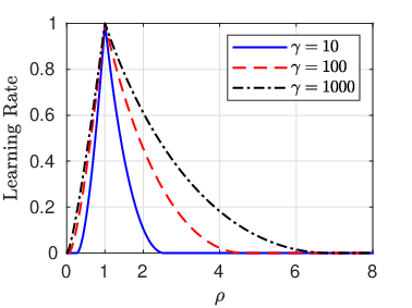
Figure 1: The learning rate 𝖤⁡(𝒫⋆,𝒬)\mathsf{E}({\cal P}^{\star},{\cal Q}) in Theorem 3 as a function of ρ\rho, for different values of γ\gamma. The maximal learning rate is achieved at ρ=1\rho=1 for any γ\gamma, as expected. Also, as γ\gamma increases the range of ρ\rho’s for which the learning rate is positive increases.

It can be checked that 𝖤⁡(𝒫⋆,𝒬)\mathsf{E}({\cal P}^{\star},{\cal Q}) is continuous in (ρ,γ)(\rho,\gamma). Theorem 3 suggests a clear phase transition in the behaviour of the learning rate (see Fig. 1 for a numerical illustration). To wit, even when players assume that the revealing probabilities decay at the same order of the optimal revealing assignments, albeit with a different constant, there are regimes where the learning rate is zero (i.e., when ρ≤ρ0\rho\leq\rho_{0} and ρ≥ρ1\rho\geq\rho_{1}). We next give a heuristic explanation as to why the learning rate is zero in these regimes. We start with the case where ρ≥ρ1\rho\geq\rho_{1}. First, note that there are two main sources for wrong action: 1) the ttth player is irrational, which happens with probability pt⋆p_{t}^{\star}, and his draw is of minority color type, or, 2) the ttth player is rational, which happens with probability 1−pt⋆1-p_{t}^{\star}, but his mismatched MAP estimate is wrong. Therefore, it is clear that the error probability can be lower bounded by 𝖯e,t​(𝒫⋆,𝒬)≥(1−pt⋆)⋅ℙ1​(𝖬𝖠𝖯𝒬​(Z1t−1,Xt)=2)\mathsf{P}_{e,t}({\cal P}^{\star},{\cal Q})\geq(1-p^{\star}_{t})\cdot\mathbb{P}_{1}\left(\mathsf{MAP}_{{\cal Q}}(Z_{1}^{t-1},X_{t})=2\right). We show in the proof that the MAP error probability can be further lower bounded by the probability that the likelihood ratio 𝖱t−1≜𝖫1t−1/𝖫2t−1\mathsf{R}_{t-1}\triangleq\mathsf{L}_{1}^{t-1}/\mathsf{L}_{2}^{t-1}, at time t−1t-1, is less than β/α\beta/\alpha, namely, we have 𝖯e,t​(𝒫⋆,𝒬)≥(1−pt⋆)⋅ℙ1​(𝖱t−1<β/α)\mathsf{P}_{e,t}({\cal P}^{\star},{\cal Q})\geq(1-p_{t}^{\star})\cdot\mathbb{P}_{1}\left(\mathsf{R}_{t-1}<\beta/\alpha\right). To further lower bound the probability term on the r.h.s. of the above inequality, we construct a particular trajectory that ensures that the likelihood ratio 𝖱t−1\mathsf{R}_{t-1} stays always below the threshold β/α\beta/\alpha. The main observation is then that when the likelihood ratio is bellow β/α\beta/\alpha, the corresponding log-likelihood ratio process log⁡𝖱t\log\mathsf{R}_{t} as a function of tt, performs a random walk with a downward drift when ρ≥ρ1\rho\geq\rho_{1}, and thus intuitively the probability that the likelihood ratio will stay bellow some fixed value is high. Technically speaking, we show that this random walk is a supermartingale, and by using well-known tail probability bounds for such processes, we show that ℙ1​(𝖱t−1<β/α)\mathbb{P}_{1}\left(\mathsf{R}_{t-1}<\beta/\alpha\right) can not decay too fast. Establishing this result, and proving a certain monotonicity property of the error probability w.r.t. 𝒬{\cal Q}, we show that 𝖤⁡(𝒫⋆,𝒬)=0\mathsf{E}({\cal P}^{\star},{\cal Q})=0 when ‖𝒬t‖≫log⁡t\left\|{\cal Q}_{t}\right\|\gg\log t as well, as claimed in Theorem 2. On other hand, when ρ<ρ1\rho<\rho_{1}, the previously mentioned random walk has an upward drift, and thus, the probability that this walk stays always bellow β/α\beta/\alpha is intuitively small, and in fact, decays at the polynomial rate given in Theorem 3.

The reason for the learning rate being zero for ρ≤ρ0\rho\leq\rho_{0} is similar. Contrary to the case where ρ≥ρ1\rho\geq\rho_{1}, in this regime, it can be shown that bellow log⁡(β/α)\log(\beta/\alpha) the log-likelihood ratio process performs a random walk with an upward drift, and thus the approach used before for lower bounding the error probability is not going to work. It turns out, however, that above log⁡(α/β)\log(\alpha/\beta), the log-likelihood ratio process has a downward drift. Moreover, we can show that in this case the walk cannot diverge, or, more precisely, go beyond a certain finite value. Among other things, this implies that it takes only a finite number of timestamps to drive the log-likelihood ratio bellow log⁡(β/α)\log(\beta/\alpha), which in turn entails that the error probability is finite as well. Specifically, to lower bound the error probability, we show that it is suffice to look at all trajectories for which the private signals of the last t⋆∈ℕt^{\star}\in\mathbb{N} revealers are opposite to the majority (e.g., Xi=2X_{i}=2, for if θ=1\theta=1). Indeed, this way we can assure that the likelihood ratio decreases by a multiplicative factor of β/α\beta/\alpha. Accordingly, since we argue that the maximal value that likelihood ratio can attain is finite, it is clear that there exists a finite value of t⋆t^{\star} which will drive 𝖱t\mathsf{R}_{t} bellow β/α\beta/\alpha (note that t⋆t^{\star} revealers decrease the likelihood by an exponential factor of (β/α)t⋆(\beta/\alpha)^{t^{\star}}). Finally, when ρ0≤ρ≤1\rho_{0}\leq\rho\leq 1, the random walk has now an upward drift, and thus, the probability that it will go bellow β/α\beta/\alpha is small, and in fact, decaying at the polynomial rate given in Theorem 3.

The above results characterize 𝖤⁡(𝒫⋆,𝒬)\mathsf{E}({\cal P}^{\star},{\cal Q}). As mentioned in the previous section, the same techniques exactly can be used to derive the learning rate 𝖤⁡(𝒫,𝒬)\mathsf{E}({\cal P},{\cal Q}) for any 𝒫{\cal P}, and we present our main findings bellow. Proof sketches can be found in Section 4.3. First, as was mentioned at the beginning of this section whenever 𝒫{\cal P} is such that ‖𝒫‖<∞\left\|{\cal P}\right\|<\infty, then Borel-Cantelli lemma implies that there will be only a finite number of revealers almost surely, which is equivalent to the situation where no revealers exist. This in turn implies a non-vanishing trivial error probability, and asymptotic learning does not occur. In fact, if ‖𝒫t‖=o⁡(log⁡t)\left\|{\cal P}_{t}\right\|=o(\log t), then 𝖤⁡(𝒫,𝒬)=0\mathsf{E}({\cal P},{\cal Q})=0, as we show in Section 4.3.

Theorem 4.

For any sequence of revealing probabilities 𝒫{\cal P} such that ‖𝒫t‖=o⁡(log⁡t)\left\|{\cal P}_{t}\right\|=o(\log t), and any sequence of mismatched revealing probabilities 𝒬{\cal Q}, it holds that 𝖤⁡(𝒫,𝒬)=0\mathsf{E}({\cal P},{\cal Q})=0.

Next, we consider the case where ‖𝒫t‖/log⁡t→𝖢𝗉\left\|{\cal P}_{t}\right\|/\log t\to\mathsf{C_{p}}, as t→∞t\to\infty, which happens to be the case, for example, when pt=𝖢𝗉/t∧1p_{t}=\mathsf{C_{p}}/t\wedge 1, for some 𝖢𝗉∈ℝ+\mathsf{C_{p}}\in\mathbb{R}_{+}. Recall the definitions of ρ0\rho_{0}, ρ1\rho_{1}, and δ⁡(γ,ρ)\delta(\gamma,\rho) in (17)–(18). We have the following result.

Theorem 5.

For any sequence of revealing probabilities 𝒫{\cal P} such that ‖𝒫t‖/log⁡t→𝖢𝗉\left\|{\cal P}_{t}\right\|/\log t\to\mathsf{C_{p}}, for some 𝖢𝗉∈ℝ+\mathsf{C_{p}}\in\mathbb{R}_{+}, and mismatched revealing probabilities 𝒬{\cal Q} such that,

lim supt→∞‖𝒬t‖‖𝒫t‖=ρ∈ℝ+,\displaystyle\limsup_{t\to\infty}\frac{\left\|{\cal Q}_{t}\right\|}{\left\|{\cal P}_{t}\right\|}=\rho\in\mathbb{R}_{+}, (20)

we have:

  • •

    If ρ≤ρ0\rho\leq\rho_{0} or ρ≥ρ1\rho\geq\rho_{1}, then

    𝖤⁡(𝒫,𝒬)=0.\mathsf{E}({\cal P},{\cal Q})=0.
  • •

    If ρ0≤ρ≤1\rho_{0}\leq\rho\leq 1,

    𝖤⁡(𝒫,𝒬)=1∧[𝖢𝗉⋅(δ⁡(γ,ρ)−γ−1γ+1​(1−ρ))].\mathsf{E}({\cal P},{\cal Q})=1\wedge\left[\mathsf{C_{p}}\cdot\left(\delta(\gamma,\rho)-\frac{\gamma-1}{\gamma+1}(1-\rho)\right)\right].
  • •

    If 1≤ρ≤ρ11\leq\rho\leq\rho_{1}, then

    𝖤⁡(𝒫,𝒬)=1∧[𝖢𝗉⋅δ⁡(γ,ρ)].\mathsf{E}({\cal P},{\cal Q})=1\wedge\left[\mathsf{C_{p}}\cdot\delta(\gamma,\rho)\right].

Refer to caption

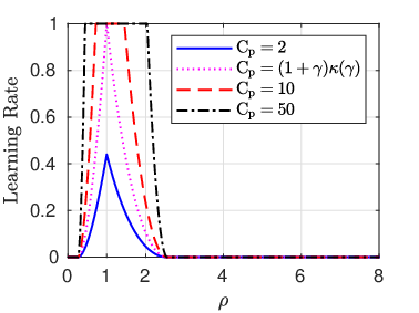
Figure 2: The learning rate 𝖤⁡(𝒫,𝒬)\mathsf{E}({\cal P},{\cal Q}) in Theorem 5 as a function of ρ\rho, for different values of 𝖢𝗉\mathsf{C_{p}}, and γ=10\gamma=10.

From Theorem 5 it can be seen that conceptually the learning rate behaves similarly to the learning rate when 𝒫=𝒫⋆{\cal P}={\cal P}^{\star}. In particular, the learning exhibits the same phase transitions as in Theorem 3. Fig. 2 presents a numerical calculation of the rate in Theorem 5, for several values of 𝖢𝗉\mathsf{C_{p}}. Note that for ρ=1\rho=1, when 𝖢𝗉<(1+γ)​κ​(γ)\mathsf{C_{p}}<(1+\gamma)\kappa(\gamma), we get that 𝖤⁡(𝒫,𝒬)<1\mathsf{E}({\cal P},{\cal Q})<1, while, for any 𝖢𝗉≥(1+γ)​κ​(γ)\mathsf{C_{p}}\geq(1+\gamma)\kappa(\gamma), we get that 𝖤⁡(𝒫,𝒬)=1\mathsf{E}({\cal P},{\cal Q})=1. This might seem counterintuitive because Theorem 1 claims that 𝖢𝗉=(1+γ)​κ​(γ)\mathsf{C_{p}}=(1+\gamma)\kappa(\gamma) is the optimal value minimizing the error probability, while the above suggests that any value 𝖢𝗉≥(1+γ)​κ​(γ)\mathsf{C_{p}}\geq(1+\gamma)\kappa(\gamma) suffices. Note, however, that while indeed any value 𝖢𝗉≥(1+γ)​κ​(γ)\mathsf{C_{p}}\geq(1+\gamma)\kappa(\gamma) gives a unit polynomial learning rate, the choice of 𝖢𝗉=(1+γ)​κ​(γ)\mathsf{C_{p}}=(1+\gamma)\kappa(\gamma) minimizes the leading coefficient in front of the decaying term, namely, lim supt→∞t⋅𝖯e,t​(𝒫⋆,𝒫⋆)<lim supt→∞t⋅𝖯e,t​(𝒫,𝒫)\limsup_{t\to\infty}t\cdot\mathsf{P}_{e,t}({\cal P}^{\star},{\cal P}^{\star})<\limsup_{t\to\infty}t\cdot\mathsf{P}_{e,t}({\cal P},{\cal P}), for any 𝒫{\cal P} with 𝖢𝗉>(1+γ)​κ​(γ)\mathsf{C_{p}}>(1+\gamma)\kappa(\gamma). This explains also why 𝖤⁡(𝒫,𝒬)\mathsf{E}({\cal P},{\cal Q}) in Theorem 5 is increasing as a function of 𝖢𝗉\mathsf{C_{p}}. Specifically, it is seen that when 𝖢𝗉>(1+γ)​κ​(γ)\mathsf{C_{p}}>(1+\gamma)\kappa(\gamma), there are values of ρ\rho for which 𝖤⁡(𝒫⋆,ρ⋅𝒫⋆)<𝖤⁡(𝒫,ρ⋅𝒫)\mathsf{E}({\cal P}^{\star},\rho\cdot{\cal P}^{\star})<\mathsf{E}({\cal P},\rho\cdot{\cal P}). Indeed, in case of mismatch, taking 𝒫⋆{\cal P}^{\star} to be the underlying revealing probabilities might be sub-optimal, and choosing a different set of probabilities which combat the mismatch results in a higher rate. Finally, we consider the case where ‖𝒫t‖=ω⁡(log⁡t)\left\|{\cal P}_{t}\right\|=\omega(\log t), for which we have the following result.

Theorem 6.

Let 𝒫{\cal P} be such that ‖𝒫t‖/log⁡t→∞\left\|{\cal P}_{t}\right\|/\log t\to\infty. If the mismatched revealing probabilities 𝒬{\cal Q} is such that,

lim supt→∞‖𝒬t‖‖𝒫t‖=ρ∈ℝ+,\displaystyle\limsup_{t\to\infty}\frac{\left\|{\cal Q}_{t}\right\|}{\left\|{\cal P}_{t}\right\|}=\rho\in\mathbb{R}_{+}, (21)

with ρ≤ρ0\rho\leq\rho_{0} or ρ≥ρ1\rho\geq\rho_{1}, or

lim inft→∞‖𝒬t‖‖𝒫t‖=0orlim supt→∞‖𝒬t‖‖𝒫t‖=∞,\liminf_{t\to\infty}\frac{\left\|{\cal Q}_{t}\right\|}{\left\|{\cal P}_{t}\right\|}=0\quad\mathrm{or}\quad\limsup_{t\to\infty}\frac{\left\|{\cal Q}_{t}\right\|}{\left\|{\cal P}_{t}\right\|}=\infty,

then 𝖤⁡(𝒫,𝒬)=0\mathsf{E}({\cal P},{\cal Q})=0. Otherwise, if ρ0<ρ<ρ1\rho_{0}<\rho<\rho_{1}, then

𝖤(𝒫,𝒬)=limt→∞−log⁡ptlog⁡t.\mathsf{E}({\cal P},{\cal Q})=\lim_{t\to\infty}-\frac{\log p_{t}}{\log t}.

Theorem 6 states that if the number of revealers is significantly bigger than log⁡t\log t, then the error probability is dominated by the probability that the ttth player is a revealer and announce a wrong decision, namely, βα+β​pt\frac{\beta}{\alpha+\beta}p_{t}. Therefore, if for example pt=Θ⁡(t−c)p_{t}=\Theta(t^{-c}), for some c∈(0,1)c\in(0,1), then 𝖤⁡(𝒫,𝒬)=c\mathsf{E}({\cal P},{\cal Q})=c, as long as the mismatch is not too “severe”, namely, ‖𝒬t‖/‖𝒫t‖→ρ\left\|{\cal Q}_{t}\right\|/\left\|{\cal P}_{t}\right\|\to\rho, and ρ0<ρ<ρ1\rho_{0}<\rho<\rho_{1}. Otherwise, learning does not occur and 𝖤⁡(𝒫,𝒬)=0\mathsf{E}({\cal P},{\cal Q})=0.

4 Proof of Main Results

4.1 Proof of Theorem 2

We start with the case where lim inft→∞‖𝒬t‖log⁡t=0\liminf_{t\to\infty}\frac{\left\|{\cal Q}_{t}\right\|}{\log t}=0. To lower bound the error probability we need to understand first how the mismatched MAP decisions evolve over time/players. We next establish some notation, which will simplify the analysis. For i∈{1,2}i\in\{1,2\} and t≥1t\geq 1, recall our notation in (4)–(8). Also, for x∈{1,2}x\in\{1,2\}, let

ϕi(x)≜αα+β𝟙[x=i]+βα+β𝟙[x≠i].\displaystyle\phi_{i}(x)\triangleq\frac{\alpha}{\alpha+\beta}\mathds{1}\left[x=i\right]+\frac{\beta}{\alpha+\beta}\mathds{1}\left[x\neq i\right]. (22)

Note that 𝖣^it=𝖫^it−1​ϕi​(Xt)\hat{\mathsf{D}}_{i}^{t}=\hat{\mathsf{L}}_{i}^{t-1}\phi_{i}(X_{t}). Finally, we define

𝖱t≜𝖫^1t𝖫^2t,𝖱t′≜𝖣^1t𝖣^2t.\displaystyle\mathsf{R}_{t}\triangleq\frac{\hat{\mathsf{L}}_{1}^{t}}{\hat{\mathsf{L}}_{2}^{t}},\quad\quad\quad\mathsf{R}^{\prime}_{t}\triangleq\frac{\hat{\mathsf{D}}_{1}^{t}}{\hat{\mathsf{D}}_{2}^{t}}. (23)

It is clear that

𝖱t′=𝖱t−1​ϕ1​(Xt)ϕ2​(Xt).\displaystyle\mathsf{R}^{\prime}_{t}=\mathsf{R}_{t-1}\frac{\phi_{1}(X_{t})}{\phi_{2}(X_{t})}. (24)

Since the ratio ϕ1​(Xt)/ϕ2​(Xt)\phi_{1}(X_{t})/\phi_{2}(X_{t}) can take values in {β/α,α/β}\{\beta/\alpha,\alpha/\beta\}, we have three possible cases only:

  • •

    If 𝖱t−1<β/α\mathsf{R}_{t-1}<\beta/\alpha then, clearly 𝖱t′<1\mathsf{R}^{\prime}_{t}<1, irrespective of the value of XtX_{t}. Thus, Zt=1Z_{t}=1 only if player tt is irrational and Xt=1X_{t}=1. Otherwise, Zt=2Z_{t}=2.

  • •

    If 𝖱t−1∈[β/α,α/β]\mathsf{R}_{t-1}\in[\beta/\alpha,\alpha/\beta] then it can be easily shown that Zt=XtZ_{t}=X_{t}.

  • •

    If 𝖱t−1>α/β\mathsf{R}_{t-1}>\alpha/\beta then, clearly 𝖱t′>1\mathsf{R}^{\prime}_{t}>1, irrespective of the value of XtX_{t}. Thus, Zt=2Z_{t}=2 only if player tt is irrational and Xt=2X_{t}=2. Otherwise, Zt=1Z_{t}=1.

Let {ℱt}t≥0\left\{{\cal F}_{t}\right\}_{t\geq 0} denote the filtration spanned by {Zt}t≥1\left\{Z_{t}\right\}_{t\geq 1}. Let ℙ^1​(Zt=i|ℱt−1)\hat{\mathbb{P}}_{1}(Z_{t}=i|{\cal F}_{t-1}) be the probability that the guess by player tt is ii, given the history and θ=1\theta=1, and the evaluation of this probability is with respect to the mismatched revealers probabilities 𝒬{\cal Q}. Then, based on the above, we have

ℙ^1​(Zt=1|ℱt−1)={αα+β​qt,if𝖱t−1<β/α,αα+β,if𝖱t−1∈[β/α,α/β],1−βα+β​qt,if𝖱t−1>α/β,\displaystyle\hat{\mathbb{P}}_{1}(Z_{t}=1|{\cal F}_{t-1})=\begin{cases}\frac{\alpha}{\alpha+\beta}q_{t},\ &\;\text{if}\quad\mathsf{R}_{t-1}<\beta/\alpha,\\ \frac{\alpha}{\alpha+\beta},\ &\;\text{if}\quad\mathsf{R}_{t-1}\in[\beta/\alpha,\alpha/\beta],\\ 1-\frac{\beta}{\alpha+\beta}q_{t},\ &\;\text{if}\quad\mathsf{R}_{t-1}>\alpha/\beta,\end{cases} (25)

and

ℙ^2​(Zt=1|ℱt−1)={βα+β​qt,if𝖱t−1<β/α,βα+β,if𝖱t−1∈[β/α,α/β],1−αα+β​qt,if𝖱t−1>α/β.\displaystyle\hat{\mathbb{P}}_{2}(Z_{t}=1|{\cal F}_{t-1})=\begin{cases}\frac{\beta}{\alpha+\beta}q_{t},\ &\;\text{if}\quad\mathsf{R}_{t-1}<\beta/\alpha,\\ \frac{\beta}{\alpha+\beta},\ &\;\text{if}\quad\mathsf{R}_{t-1}\in[\beta/\alpha,\alpha/\beta],\\ 1-\frac{\alpha}{\alpha+\beta}q_{t},\ &\;\text{if}\quad\mathsf{R}_{t-1}>\alpha/\beta.\end{cases} (26)

There are two main sources for wrong action: 1) the ttth player is irrational, which happens with probability ptp_{t}, and his draw is of minority color type, or, 2) the ttth player is rational, but his mismatched MAP estimate is wrong. Accordingly, we can write

𝖯e,t​(𝒫⋆,𝒬)\displaystyle\mathsf{P}_{e,t}({\cal P}^{\star},{\cal Q}) =ℙ⁡(𝖬𝖠𝖯𝒬​(Z1t−1,Xt)≠θ)⋅(1−pt⋆)+ℙ⁡(Xt≠θ)⋅pt⋆\displaystyle=\mathbb{P}\left(\mathsf{MAP}_{{\cal Q}}(Z_{1}^{t-1},X_{t})\neq\theta\right)\cdot(1-p^{\star}_{t})+\mathbb{P}(X_{t}\neq\theta)\cdot p^{\star}_{t}
≥ℙ⁡(𝖬𝖠𝖯𝒬​(Z1t−1,Xt)≠θ)⋅(1−pt⋆)\displaystyle\geq\mathbb{P}\left(\mathsf{MAP}_{{\cal Q}}(Z_{1}^{t-1},X_{t})\neq\theta\right)\cdot(1-p^{\star}_{t})
=ℙ1​(𝖬𝖠𝖯𝒬​(Z1t−1,Xt)=2)⋅(1−pt⋆),\displaystyle=\mathbb{P}_{1}\left(\mathsf{MAP}_{{\cal Q}}(Z_{1}^{t-1},X_{t})=2\right)\cdot(1-p^{\star}_{t}), (27)

where the last equality follows by symmetry. We next lower bound the probability term at the r.h.s. of (27). To this end, we define an event that implies that the output of the mismatched MAP is 22, given that θ=1\theta=1. Let t¯1,t¯2≤t⋆\bar{t}_{1},\bar{t}_{2}\leq t^{\star} be three natural numbers, to be defined in the sequel. Let 𝗋𝖾𝗏⁡(t⋆)≜{i1,i2,…,it⋆}\mathsf{rev}(t^{\star})\triangleq\left\{i_{1},i_{2},\ldots,i_{t^{\star}}\right\} be the set of the last t⋆t^{\star} revealers. Define the following event

ℰ⁡(t¯1,t¯2,t⋆)\displaystyle{\cal E}(\bar{t}_{1},\bar{t}_{2},t^{\star}) ≜{Xi=2,∀i∈𝗋𝖾𝗏(t⋆)∪{it¯1,it¯1+1…,it¯1+t¯2}},\displaystyle\triangleq\left\{X_{i}=2,\forall i\in\mathsf{rev}(t^{\star})\cup\left\{i_{\bar{t}_{1}},i_{\bar{t}_{1}}+1\ldots,i_{\bar{t}_{1}}+\bar{t}_{2}\right\}\right\}, (28)

namely, it is the event that the last t⋆t^{\star} revealers are such that their private signal is “22”, and all consecutive players it¯1,it¯1+1,…,it¯1+t¯2i_{\bar{t}_{1}},i_{\bar{t}_{1}}+1,\ldots,i_{\bar{t}_{1}}+\bar{t}_{2} (either revealers or rationals) are such that their private signal is “22” as well. We claim that by carefully choosing the values of t¯1\bar{t}_{1}, t¯2\bar{t}_{2}, and t⋆t^{\star}, we can show that ℰ⁡(t¯1,t¯2,t⋆){\cal E}(\bar{t}_{1},\bar{t}_{2},t^{\star}) implies that the ttth player (mismatched MAP) guess is “22”. To this end, note that the first two individuals follow their private signals, that is Z1=X1Z_{1}=X_{1} and Z2=X2Z_{2}=X_{2}. Therefore, if X1=X2=1X_{1}=X_{2}=1, then 𝖱2=(α/β)2\mathsf{R}_{2}=(\alpha/\beta)^{2}, otherwise, 𝖱2=(β/α)2\mathsf{R}_{2}=(\beta/\alpha)^{2}. Depending on either one of the above situations, the proceeding guesses depend on whether a student is a revealer or not, and value of the likelihood 𝖱t\mathsf{R}_{t} at each step tt. Accordingly, at step i1−1i_{1}-1, the worst-case (largest) attainable value of the likelihood ratio is

𝖱i1−1\displaystyle\mathsf{R}_{i_{1}-1} =(αβ)2⋅∏i=3i1−11−βα−β​qi1−αα−β​qi\displaystyle=\left(\frac{\alpha}{\beta}\right)^{2}\cdot\prod_{i=3}^{i_{1}-1}\frac{1-\frac{\beta}{\alpha-\beta}q_{i}}{1-\frac{\alpha}{\alpha-\beta}q_{i}} (29)
≤(αβ)2​eα−βα+β​∑i=3i1−1qi,\displaystyle\leq\left(\frac{\alpha}{\beta}\right)^{2}e^{\frac{\alpha-\beta}{\alpha+\beta}\sum_{i=3}^{i_{1}-1}q_{i}}, (30)

which corresponds to the situation where X1=X2=1X_{1}=X_{2}=1, and the proceeding players decisions up to t≤i1−1t\leq i_{1}-1 are Zt=1Z_{t}=1. Now, over ℰ⁡(t¯1,t¯2,t⋆){\cal E}(\bar{t}_{1},\bar{t}_{2},t^{\star}), we know that the i1i_{1} player is a revealer and its private information is Xi1=2X_{i_{1}}=2. Since he is a revealer its decision will be Zi1=2Z_{i_{1}}=2, which implies that the likelihood ratio is

𝖱i1=(αβ)⋅∏i=3i1−11−βα−β​qi1−αα−β​qi.\displaystyle\mathsf{R}_{i_{1}}=\left(\frac{\alpha}{\beta}\right)\cdot\prod_{i=3}^{i_{1}-1}\frac{1-\frac{\beta}{\alpha-\beta}q_{i}}{1-\frac{\alpha}{\alpha-\beta}q_{i}}. (31)

The index of the next revealer is i2i_{2}. Thus, since 𝖱i1>α/β\mathsf{R}_{i_{1}}>\alpha/\beta, the decisions of the proceeding players up to player i2i_{2}, are “11”, which imply that

𝖱i2−1=(αβ)⋅∏i=3i2−11−βα−β​qi1−αα−β​qi.\displaystyle\mathsf{R}_{i_{2}-1}=\left(\frac{\alpha}{\beta}\right)\cdot\prod_{i=3}^{i_{2}-1}\frac{1-\frac{\beta}{\alpha-\beta}q_{i}}{1-\frac{\alpha}{\alpha-\beta}q_{i}}. (32)

Then, since i2i_{2} is a revealer and its private information is Xi2=2X_{i_{2}}=2, we have

𝖱i2=∏i=3i1−11−βα−β​qi1−αα−β​qi,\displaystyle\mathsf{R}_{i_{2}}=\prod_{i=3}^{i_{1}-1}\frac{1-\frac{\beta}{\alpha-\beta}q_{i}}{1-\frac{\alpha}{\alpha-\beta}q_{i}}, (33)

and the above process continues. In particular, assuming that 𝖱ij−1>α/β\mathsf{R}_{i_{j-1}}>\alpha/\beta, the likelihood ratio after the iji_{j}th decision is

𝖱ij=(βα)j−2​∏i=3ij−11−βα−β​qi1−αα−β​qi.\displaystyle\mathsf{R}_{i_{j}}=\left(\frac{\beta}{\alpha}\right)^{j-2}\prod_{i=3}^{i_{j}-1}\frac{1-\frac{\beta}{\alpha-\beta}q_{i}}{1-\frac{\alpha}{\alpha-\beta}q_{i}}. (34)

We denote by t¯1\bar{t}_{1} the index at which the likelihood ratio 𝖱it¯1\mathsf{R}_{i_{\bar{t}_{1}}}, after the it¯1i_{\bar{t}_{1}}th decision, is in the interval [β/α,α/β]\left[\beta/\alpha,\alpha/\beta\right]. Indeed, when this happens, according to (25)–(26), the likelihood ratio 𝖱it¯1\mathsf{R}_{i_{\bar{t}_{1}}} will be multiplied by either β/α\beta/\alpha or α/β\alpha/\beta depending on whether the private information is “22” or “11”, respectively, until the likelihood ratio value will be either below β/α\beta/\alpha or above α/β\alpha/\beta. Accordingly, over ℰ⁡(t¯1,t¯2,t⋆){\cal E}(\bar{t}_{1},\bar{t}_{2},t^{\star}), we force the private information of players it¯1,it¯1+1,…,it¯1+t¯2i_{\bar{t}_{1}},i_{\bar{t}_{1}}+1,\ldots,i_{\bar{t}_{1}}+\bar{t}_{2} to be “22”, so that the corresponding likelihoods will be multiplied by β/α\beta/\alpha, until the likelihood ratio value will get bellow β/α\beta/\alpha, and accordingly, t¯2\bar{t}_{2} is chosen such that

𝖱t¯1+t¯2=(βα)t¯1+t¯2−2​∏i=3it¯−11−βα−β​qi1−αα−β​qi,\displaystyle\mathsf{R}_{\bar{t}_{1}+\bar{t}_{2}}=\left(\frac{\beta}{\alpha}\right)^{\bar{t}_{1}+\bar{t}_{2}-2}\prod_{i=3}^{i_{\bar{t}}-1}\frac{1-\frac{\beta}{\alpha-\beta}q_{i}}{1-\frac{\alpha}{\alpha-\beta}q_{i}}, (35)

will be less than β/α\beta/\alpha. Next, due to the fact that over ℰ⁡(t¯1,t¯2,t⋆){\cal E}(\bar{t}_{1},\bar{t}_{2},t^{\star}) the leftover revealers are such that their private information is “22”, and the likelihood ratio is below β/α\beta/\alpha (and so MAP outputs “22”), it is clear that all the leftover players decisions will be “22”. To assure that we take enough revealers at the end, we chose t⋆t^{\star} such that,

(βα)t⋆−2​∏i=3t−t∗1−βα−β​qi1−αα−β​qi<βα,\displaystyle\left(\frac{\beta}{\alpha}\right)^{t^{\star}-2}\prod_{i=3}^{t-t^{*}}\frac{1-\frac{\beta}{\alpha-\beta}q_{i}}{1-\frac{\alpha}{\alpha-\beta}q_{i}}<\frac{\beta}{\alpha}, (36)

which reflects the case where the players decision are always “11” up to time t−t⋆t-t^{\star}, and then the left over t⋆t^{\star} players are all revealers with “22” being their private information. It is evident that (36) holds if

t⋆≥3+α−βα+β⋅‖𝒬t‖log⁡(α/β).\displaystyle t^{\star}\geq 3+\frac{\alpha-\beta}{\alpha+\beta}\cdot\frac{\left\|{\cal Q}_{t}\right\|}{\log(\alpha/\beta)}. (37)

Note that when ‖𝒬t‖\left\|{\cal Q}_{t}\right\| is a finite number which happens to be the case when qt=o⁡(t−1)q_{t}=o(t^{-1}) (as opposed to ‖𝒫t⋆‖\left\|{\cal P}^{\star}_{t}\right\| which grows logarithmically with tt), implies that t⋆t^{\star} is finite, which in turn is the reason for the fact that the error probability is finite. Also, by the same token, it is clear that t¯1\bar{t}_{1} and t¯2\bar{t}_{2} are finite too, with t¯2<t⋆\bar{t}_{2}<t^{\star}. The latter implies that ℰ⁡(t¯1,t⋆,t⋆)⊆ℰ⁡(t¯1,t¯2,t⋆){\cal E}(\bar{t}_{1},t^{\star},t^{\star})\subseteq{\cal E}(\bar{t}_{1},\bar{t}_{2},t^{\star}). Finally, we need to make sure that the size of the set of all revealers, denoted by 𝖱𝖾𝗏t≜{i∈[t]:player ​i​ is revealer}\mathsf{Rev}_{t}\triangleq\{i\in[t]:\text{player }i\text{ is revealer}\} is bigger than t⋆t^{\star} with high probability. Let Mt≜∑i=1tpi∼log⁡tM_{t}\triangleq\sum_{i=1}^{t}p_{i}\sim\log t. Then, by Chernoff’s bound ℙ⁡(|𝖱𝖾𝗏t|≤t⋆)≤exp⁡(t⋆​log⁡Mtt⋆−Mt+t⋆)=O⁡(t−1)≤1/2\mathbb{P}\left(\left|\mathsf{Rev}_{t}\right|\leq t^{\star}\right)\leq\exp(t^{\star}\log\frac{M_{t}}{t^{\star}}-M_{t}+t^{\star})=O(t^{-1})\leq 1/2. Thus, we get that

ℙ1​(𝖬𝖠𝖯𝒬​(Z1t−1,Xt)=2)≥ℙ1​[ℰ⁡(t¯1,t¯2,t⋆)]\displaystyle\mathbb{P}_{1}\left(\mathsf{MAP}_{{\cal Q}}(Z_{1}^{t-1},X_{t})=2\right)\geq\mathbb{P}_{1}\left[{\cal E}(\bar{t}_{1},\bar{t}_{2},t^{\star})\right] ≥∑𝒜:|𝒜|>t⋆ℙ(𝖱𝖾𝗏t=𝒜)ℙ1[ℰ(t¯1,t¯2,t⋆)|𝖱𝖾𝗏t=𝒜]\displaystyle\geq\sum_{{\cal A}:|{\cal A}|>t^{\star}}\mathbb{P}\left(\mathsf{Rev}_{t}={\cal A}\right)\mathbb{P}_{1}\left[\left.{\cal E}(\bar{t}_{1},\bar{t}_{2},t^{\star})\right|\mathsf{Rev}_{t}={\cal A}\right]
≥∑𝒜:|𝒜|>t⋆ℙ(𝖱𝖾𝗏t=𝒜)ℙ1[ℰ(t¯1,t⋆,t⋆)|𝖱𝖾𝗏t=𝒜]\displaystyle\geq\sum_{{\cal A}:|{\cal A}|>t^{\star}}\mathbb{P}\left(\mathsf{Rev}_{t}={\cal A}\right)\mathbb{P}_{1}\left[\left.{\cal E}(\bar{t}_{1},t^{\star},t^{\star})\right|\mathsf{Rev}_{t}={\cal A}\right]
≥(βα+β)2​t⋆⋅ℙ⁡(|𝖱𝖾𝗏t|>t⋆)\displaystyle\geq\left(\frac{\beta}{\alpha+\beta}\right)^{2t^{\star}}\cdot\mathbb{P}\left(|\mathsf{Rev}_{t}|>t^{\star}\right)
≥12​(βα+β)2​t⋆.\displaystyle\geq\frac{1}{2}\left(\frac{\beta}{\alpha+\beta}\right)^{2t^{\star}}. (38)

Therefore, using (27), (38), and the fact that lim inft→∞‖𝒬t‖log⁡t=0\liminf_{t\to\infty}\frac{\left\|{\cal Q}_{t}\right\|}{\log t}=0 we get

𝖤⁡(𝒫⋆,𝒬)\displaystyle\mathsf{E}({\cal P}^{\star},{\cal Q}) =lim inft→∞−log⁡𝖯e,t​(𝒫⋆,𝒬)log⁡t\displaystyle=\liminf_{t\to\infty}-\frac{\log\mathsf{P}_{e,t}({\cal P}^{\star},{\cal Q})}{\log t} (39)
≤2​log⁡(α+ββ)⋅lim inft→∞t⋆log⁡t=0.\displaystyle\leq 2\log\left(\frac{\alpha+\beta}{\beta}\right)\cdot\liminf_{t\to\infty}\frac{t^{\star}}{\log t}=0. (40)

Since it is clear that 𝖤⁡(𝒫⋆,𝒬)≥0\mathsf{E}({\cal P}^{\star},{\cal Q})\geq 0 we may conclude that in this regime 𝖤⁡(𝒫⋆,𝒬)=0\mathsf{E}({\cal P}^{\star},{\cal Q})=0. Finally, proving that 𝖤⁡(𝒫⋆,𝒬)=0\mathsf{E}({\cal P}^{\star},{\cal Q})=0 for the case lim inft→∞‖𝒬t‖log⁡t=∞\liminf_{t\to\infty}\frac{\left\|{\cal Q}_{t}\right\|}{\log t}=\infty follows from Theorem 3 (specifically, using the fact that for ρ>ρ1\rho>\rho_{1} we have 𝖤⁡(𝒫⋆,𝒬)=0\mathsf{E}({\cal P}^{\star},{\cal Q})=0), and a monotonicity property of the error probability w.r.t. the revealing probabilities 𝒬{\cal Q}. We provide the complete details in Section 4.2.2.

4.2 Proof of Theorem 3

We split the proofs into several upper and lower bounds, which together characterize tightly the asymptotic learning rate. Note that by “lower bounds” (“upper bounds”) we mean lower- (upper-) bounding the learning rate by upper- (lower-) bounding the error probability.

4.2.1 Lower Bound: ρ0≤ρ≤ρ1\rho_{0}\leq\rho\leq\rho_{1}

We analyze next the probability of wrong action by the ttth player. Accordingly, there are two main sources for wrong action: 1) the ttth player is irrational, which happens with probability ptp_{t}, and his draw is of minority color type, or, 2) the ttth player is rational, but his mismatched MAP estimate is wrong. Accordingly, we can write

𝖯e,t​(𝒫,𝒬)\displaystyle\mathsf{P}_{e,t}({\cal P},{\cal Q}) =ℙ⁡(𝖬𝖠𝖯𝒬​(Z1t−1,Xt)≠θ)⋅(1−pt)+ℙ⁡(Xt≠θ)⋅pt\displaystyle=\mathbb{P}\left(\mathsf{MAP}_{{\cal Q}}(Z_{1}^{t-1},X_{t})\neq\theta\right)\cdot(1-p_{t})+\mathbb{P}(X_{t}\neq\theta)\cdot p_{t} (41)
=ℙ⁡(𝖬𝖠𝖯𝒬​(Z1t−1,Xt)≠θ)⋅(1−pt)+βα+β⋅pt.\displaystyle=\mathbb{P}\left(\mathsf{MAP}_{{\cal Q}}(Z_{1}^{t-1},X_{t})\neq\theta\right)\cdot(1-p_{t})+\frac{\beta}{\alpha+\beta}\cdot p_{t}. (42)

Therefore, to upper bound 𝖯e,t​(𝒫,𝒬)\mathsf{P}_{e,t}({\cal P},{\cal Q}) we need to upper bound the probability that the mismatched MAP estimator is incorrect. To this end, we next establish some notation, which will simplify the analysis. For i∈{1,2}i\in\{1,2\} and t≥1t\geq 1, recall our notations in (4)–(8), as well as the definitions in (22)–(24). Finally, recall that depending on the value that 𝖱t−1\mathsf{R}_{t-1} takes, there are three modes of operation for the MAP estimator (see, the paragraph following (24)). In particular, the error probability associated with the MAP estimator can be upper bounded as follows,

ℙ⁡(𝖬𝖠𝖯𝒬​(Z1t−1,Xt)≠θ)\displaystyle\mathbb{P}\left(\mathsf{MAP}_{{\cal Q}}(Z_{1}^{t-1},X_{t})\neq\theta\right) =ℙ1​(𝖬𝖠𝖯𝒬​(Z1t−1,Xt)≠1)\displaystyle=\mathbb{P}_{1}\left(\mathsf{MAP}_{{\cal Q}}(Z_{1}^{t-1},X_{t})\neq 1\right)
=ℙ1​(𝖱t′≤1)\displaystyle=\mathbb{P}_{1}\left(\mathsf{R}^{\prime}_{t}\leq 1\right)
≤ℙ1​(𝖱t−1≤αβ).\displaystyle\leq\mathbb{P}_{1}\left(\mathsf{R}_{t-1}\leq\frac{\alpha}{\beta}\right). (43)

Thus, it is suffice to upper bound ℙ1​(𝖱t−1≤α/β)\mathbb{P}_{1}\left(\mathsf{R}_{t-1}\leq\alpha/\beta\right). To this end, we use similar techniques used in [17, Sec. 2.2], but with modifications which handle the mismatch aspect of our model. Let {ℱt}t≥0\left\{{\cal F}_{t}\right\}_{t\geq 0} denote the filtration spanned by {Zt}t≥1\left\{Z_{t}\right\}_{t\geq 1}. Then, for λ∈[0,1]\lambda\in[0,1], we have

𝔼1[(𝖱t𝖱t−1)−λ|ℱt−1]\displaystyle\mathbb{E}_{1}\left[\left.\left(\frac{\mathsf{R}_{t}}{\mathsf{R}_{t-1}}\right)^{-\lambda}\right|{\cal F}_{t-1}\right] =𝔼1[(ℙ^1​(Zt|ℱt−1)ℙ^2​(Zt|ℱt−1))−λ|ℱt−1]\displaystyle=\mathbb{E}_{1}\left[\left.\left(\frac{\hat{\mathbb{P}}_{1}(Z_{t}|{\cal F}_{t-1})}{\hat{\mathbb{P}}_{2}(Z_{t}|{\cal F}_{t-1})}\right)^{-\lambda}\right|{\cal F}_{t-1}\right] (44)
=∑i∈{1,2}ℙ1​(Zt=i|ℱt−1)​(ℙ^1​(Zt=i|ℱt−1)ℙ^2​(Zt=i|ℱt−1))−λ,\displaystyle=\sum_{i\in\{1,2\}}\mathbb{P}_{1}(Z_{t}=i|{\cal F}_{t-1})\left(\frac{\hat{\mathbb{P}}_{1}(Z_{t}=i|{\cal F}_{t-1})}{\hat{\mathbb{P}}_{2}(Z_{t}=i|{\cal F}_{t-1})}\right)^{-\lambda}, (45)

where ℙ1​(Zt=i|ℱt−1)\mathbb{P}_{1}(Z_{t}=i|{\cal F}_{t-1}) is the probability that player tt guess is ii given the history and θ=1\theta=1, and the evaluation of this probability is with respect to the underlying true revealers probabilities 𝒫{\cal P}. On the other hand, ℙ^1​(Zt=i|ℱt−1)\hat{\mathbb{P}}_{1}(Z_{t}=i|{\cal F}_{t-1}) is the probability that player tt guess is ii given the history and θ=1\theta=1, and the evaluation of this probability is with respect to the mismatched revealers probabilities 𝒬{\cal Q}. Accordingly, the values of these probabilities are given in (25)–(26), and

ℙ1​(Zt=1|ℱt−1)\displaystyle\mathbb{P}_{1}(Z_{t}=1|{\cal F}_{t-1}) ={αα+β​pt,if𝖱t−1<β/α,αα+β,if𝖱t−1∈[β/α,α/β],1−βα+β​pt,if𝖱t−1>α/β.\displaystyle=\begin{cases}\frac{\alpha}{\alpha+\beta}p_{t},\ &\;\text{if}\quad\mathsf{R}_{t-1}<\beta/\alpha,\\ \frac{\alpha}{\alpha+\beta},\ &\;\text{if}\quad\mathsf{R}_{t-1}\in[\beta/\alpha,\alpha/\beta],\\ 1-\frac{\beta}{\alpha+\beta}p_{t},\ &\;\text{if}\quad\mathsf{R}_{t-1}>\alpha/\beta.\end{cases} (46)

Therefore, we have,

𝔼1[(𝖱t𝖱t−1)−λ|ℱt−1,𝖱t−1<βα]\displaystyle\mathbb{E}_{1}\left[\left.\left(\frac{\mathsf{R}_{t}}{\mathsf{R}_{t-1}}\right)^{-\lambda}\right|{\cal F}_{t-1},\mathsf{R}_{t-1}<\frac{\beta}{\alpha}\right] =α1−λ​βλα+β​pt+(1−αα+β​pt)​[1−βα+β​qt1−αα+β​qt]λ,\displaystyle=\frac{\alpha^{1-\lambda}\beta^{\lambda}}{\alpha+\beta}p_{t}+\left(1-\frac{\alpha}{\alpha+\beta}p_{t}\right)\left[\frac{1-\frac{\beta}{\alpha+\beta}q_{t}}{1-\frac{\alpha}{\alpha+\beta}q_{t}}\right]^{\lambda}, (47)
𝔼1[(𝖱t𝖱t−1)−λ|ℱt−1,𝖱t−1∈[βα,αβ]]\displaystyle\mathbb{E}_{1}\left[\left.\left(\frac{\mathsf{R}_{t}}{\mathsf{R}_{t-1}}\right)^{-\lambda}\right|{\cal F}_{t-1},\mathsf{R}_{t-1}\in\left[\frac{\beta}{\alpha},\frac{\alpha}{\beta}\right]\right] =α1−λ​βλ+αλ​β1−λα+β,\displaystyle=\frac{\alpha^{1-\lambda}\beta^{\lambda}+\alpha^{\lambda}\beta^{1-\lambda}}{\alpha+\beta}, (48)
𝔼1[(𝖱t𝖱t−1)−λ|ℱt−1,𝖱t−1>αβ]\displaystyle\mathbb{E}_{1}\left[\left.\left(\frac{\mathsf{R}_{t}}{\mathsf{R}_{t-1}}\right)^{-\lambda}\right|{\cal F}_{t-1},\mathsf{R}_{t-1}>\frac{\alpha}{\beta}\right] =αλ​β1−λα+β​pt+(1−βα+β​pt)​[1−αα+β​qt1−βα+β​qt]λ.\displaystyle=\frac{\alpha^{\lambda}\beta^{1-\lambda}}{\alpha+\beta}p_{t}+\left(1-\frac{\beta}{\alpha+\beta}p_{t}\right)\left[\frac{1-\frac{\alpha}{\alpha+\beta}q_{t}}{1-\frac{\beta}{\alpha+\beta}q_{t}}\right]^{\lambda}. (49)

Since we assume that both ptp_{t} and qtq_{t} decay with tt, we use the fact that (1−δ)λ=1−λ⋅δ+Θ⁡(δ2)(1-\delta)^{\lambda}=1-\lambda\cdot\delta+\Theta(\delta^{2}), as δ→0\delta\to 0. Let

fλ\displaystyle f_{\lambda} ≡fλ​(α,β)≜α−α1−λ​βλα+β,\displaystyle\equiv f_{\lambda}(\alpha,\beta)\triangleq\frac{\alpha-\alpha^{1-\lambda}\beta^{\lambda}}{\alpha+\beta}, (50)
gλ\displaystyle g_{\lambda} ≡gλ​(α,β)≜(α−β)​λα+β,\displaystyle\equiv g_{\lambda}(\alpha,\beta)\triangleq\frac{(\alpha-\beta)\lambda}{\alpha+\beta}, (51)
hλ\displaystyle h_{\lambda} ≡hλ​(α,β)≜β−αλ​β1−λα+β.\displaystyle\equiv h_{\lambda}(\alpha,\beta)\triangleq\frac{\beta-\alpha^{\lambda}\beta^{1-\lambda}}{\alpha+\beta}. (52)

Then, we have

𝔼1[(𝖱t𝖱t−1)−λ|ℱt−1,𝖱t−1<βα]=1−fλ⋅pt+gλ⋅qt+O(pt2+qt2),\displaystyle\mathbb{E}_{1}\left[\left.\left(\frac{\mathsf{R}_{t}}{\mathsf{R}_{t-1}}\right)^{-\lambda}\right|{\cal F}_{t-1},\mathsf{R}_{t-1}<\frac{\beta}{\alpha}\right]=1-f_{\lambda}\cdot p_{t}+g_{\lambda}\cdot q_{t}+O(p_{t}^{2}+q_{t}^{2}), (53)
𝔼1[(𝖱t𝖱t−1)−λ|ℱt−1,𝖱t−1∈[βα,αβ]]=α1−λ​βλ+αλ​β1−λα+β,\displaystyle\mathbb{E}_{1}\left[\left.\left(\frac{\mathsf{R}_{t}}{\mathsf{R}_{t-1}}\right)^{-\lambda}\right|{\cal F}_{t-1},\mathsf{R}_{t-1}\in\left[\frac{\beta}{\alpha},\frac{\alpha}{\beta}\right]\right]=\frac{\alpha^{1-\lambda}\beta^{\lambda}+\alpha^{\lambda}\beta^{1-\lambda}}{\alpha+\beta}, (54)
𝔼1[(𝖱t𝖱t−1)−λ|ℱt−1,𝖱t−1>αβ]=1−hλ⋅pt−gλ⋅qt+O(pt2+qt2).\displaystyle\mathbb{E}_{1}\left[\left.\left(\frac{\mathsf{R}_{t}}{\mathsf{R}_{t-1}}\right)^{-\lambda}\right|{\cal F}_{t-1},\mathsf{R}_{t-1}>\frac{\alpha}{\beta}\right]=1-h_{\lambda}\cdot p_{t}-g_{\lambda}\cdot q_{t}+O(p_{t}^{2}+q_{t}^{2}). (55)

Define the following two sets:

𝒜t≜{i∈[t]:𝖱i−1>αβ},\displaystyle{\cal A}_{t}\triangleq\left\{i\in[t]:\mathsf{R}_{i-1}>\frac{\alpha}{\beta}\right\}, (56)

and ℬt≜𝒜tc=[t]∖𝒜t{\cal B}_{t}\triangleq{\cal A}_{t}^{c}=[t]\setminus{\cal A}_{t}. Define also,

𝖱t(1)≜∏i∈𝒜t𝖱i𝖱i−1\displaystyle\mathsf{R}_{t}^{(1)}\triangleq\prod_{i\in{\cal A}_{t}}\frac{\mathsf{R}_{i}}{\mathsf{R}_{i-1}} (57)

and

𝖱t(2)≜∏i∈ℬt𝖱i𝖱i−1.\displaystyle\mathsf{R}_{t}^{(2)}\triangleq\prod_{i\in{\cal B}_{t}}\frac{\mathsf{R}_{i}}{\mathsf{R}_{i-1}}. (58)

Note that 𝖱t=𝖱t(1)⋅𝖱t(2)\mathsf{R}_{t}=\mathsf{R}_{t}^{(1)}\cdot\mathsf{R}_{t}^{(2)}. We these definitions, using (53)–(55), we note that there exist some constants CC and C′C^{\prime} independent of λ\lambda, such that for all λ\lambda,

𝔼1[(𝖱t𝖱t−1)−λehλ​pt+gλ​qt|𝖱t−1,t∈𝒜t]≤eC′​(pt2+qt2),\displaystyle\mathbb{E}_{1}\left[\left.\left(\frac{\mathsf{R}_{t}}{\mathsf{R}_{t-1}}\right)^{-\lambda}e^{h_{\lambda}p_{t}+g_{\lambda}q_{t}}\right|\mathsf{R}_{t-1},t\in{\cal A}_{t}\right]\leq e^{C^{\prime}(p_{t}^{2}+q_{t}^{2})}, (59)

and

𝔼1[(𝖱t𝖱t−1)−λefλ​pt−gλ​qt|𝖱t−1,t∈ℬt]≤eC⁡(pt2+qt2).\displaystyle\mathbb{E}_{1}\left[\left.\left(\frac{\mathsf{R}_{t}}{\mathsf{R}_{t-1}}\right)^{-\lambda}e^{f_{\lambda}p_{t}-g_{\lambda}q_{t}}\right|\mathsf{R}_{t-1},t\in{\cal B}_{t}\right]\leq e^{C(p_{t}^{2}+q_{t}^{2})}. (60)

Recall that ‖𝒫t‖=∑i=1tpi\left\|{\cal P}_{t}\right\|=\sum_{i=1}^{t}p_{i} and ‖𝒬t‖=∑i=1tqi\left\|{\cal Q}_{t}\right\|=\sum_{i=1}^{t}q_{i}. Also, let Γtp≜∑i∈𝒜ttpi\Gamma_{t}^{p}\triangleq\sum_{i\in{\cal A}_{t}}^{t}p_{i} and Γtq≜∑i∈𝒜ttqi\Gamma_{t}^{q}\triangleq\sum_{i\in{\cal A}_{t}}^{t}q_{i}. By induction, we can easily see that there exists a constant CC such that for any λ1,λ2∈[0,1]\lambda_{1},\lambda_{2}\in[0,1],

𝔼1​[(𝖱t(1))−λ1​ehλ1​Γtp+gλ1​Γtq​(𝖱t(2))−λ2​efλ2​(‖𝒫t‖−Γtp)−gλ2​(‖𝒬t‖−Γtq)]≤eC​∑i=1t(pi2+qi2),\displaystyle\mathbb{E}_{1}\left[\left(\mathsf{R}_{t}^{(1)}\right)^{-\lambda_{1}}e^{h_{\lambda_{1}}\Gamma_{t}^{p}+g_{\lambda_{1}}\Gamma_{t}^{q}}\left(\mathsf{R}_{t}^{(2)}\right)^{-\lambda_{2}}\vphantom{\left(\mathsf{R}_{t}^{(1)}\right)^{-\lambda_{1}}}e^{f_{\lambda_{2}}(\left\|{\cal P}_{t}\right\|-\Gamma_{t}^{p})-g_{\lambda_{2}}(\left\|{\cal Q}_{t}\right\|-\Gamma_{t}^{q})}\right]\leq e^{C\sum_{i=1}^{t}(p_{i}^{2}+q_{i}^{2})}, (61)

and since ∑i=1t(pi2+qi2)\sum_{i=1}^{t}(p_{i}^{2}+q_{i}^{2}) is finite, we can upper bound the r.h.s. of (61) by a constant C0C_{0}. Now, as was shown in [17, Appendix A], the condition 𝖱t≤αβ\mathsf{R}_{t}\leq\frac{\alpha}{\beta} implies that 𝖱t(1)≤1\mathsf{R}_{t}^{(1)}\leq 1. Thus, we may write

ℙ1​(𝖱t≤αβ)\displaystyle\mathbb{P}_{1}\left(\mathsf{R}_{t}\leq\frac{\alpha}{\beta}\right) ≤ℙ1(𝖱t≤αβ,t−C1≤𝖱t(1)≤1)+ℙ1(𝖱t(1)≤t−C1).\displaystyle\leq\mathbb{P}_{1}\left(\mathsf{R}_{t}\leq\frac{\alpha}{\beta},\;t^{-C_{1}}\leq\mathsf{R}_{t}^{(1)}\leq 1\right)+\mathbb{P}_{1}\left(\mathsf{R}_{t}^{(1)}\leq t^{-C_{1}}\right). (62)

A simple application of multiplicative Chrenoff’s bound shows that the second term on the r.h.s. of the above inequality is upper bounded by t−2t^{-2}, for some constant C1<∞C_{1}<\infty. We next upper bound the first term on the r.h.s. of the above inequality. Since 𝖱t=𝖱t(1)⋅𝖱t(2)\mathsf{R}_{t}=\mathsf{R}_{t}^{(1)}\cdot\mathsf{R}_{t}^{(2)}, we can write

ℙ1(𝖱t≤αβ,t−C1≤𝖱t(1)≤1)\displaystyle\mathbb{P}_{1}\left(\mathsf{R}_{t}\leq\frac{\alpha}{\beta},\;t^{-C_{1}}\leq\mathsf{R}_{t}^{(1)}\leq 1\right) ≤∑x=0C1​log⁡tℙ1​(𝖱t(1)∈[e−(x+1),e−x],𝖱t(2)≤ex+C3)\displaystyle\leq\sum_{x=0}^{C_{1}\log t}\mathbb{P}_{1}\left(\mathsf{R}_{t}^{(1)}\in\left[e^{-(x+1)},e^{-x}\right],\mathsf{R}_{t}^{(2)}\leq e^{x+C_{3}}\right) (63)
≤∑x=0C1​log⁡tℙ1​(𝖱t(1)≤e−x,𝖱t(2)≤ex+C3),\displaystyle\leq\sum_{x=0}^{C_{1}\log t}\mathbb{P}_{1}\left(\mathsf{R}_{t}^{(1)}\leq e^{-x},\mathsf{R}_{t}^{(2)}\leq e^{x+C_{3}}\right), (64)

where C3≜1+log⁡αβC_{3}\triangleq 1+\log\frac{\alpha}{\beta}. Then, for any λ1,λ2∈[0,1]\lambda_{1},\lambda_{2}\in[0,1], we have

ℙ1​(𝖱t(1)≤e−x,𝖱t(2)≤ex+C3)\displaystyle\mathbb{P}_{1}\left(\mathsf{R}_{t}^{(1)}\leq e^{-x},\mathsf{R}_{t}^{(2)}\leq e^{x+C_{3}}\right) =ℙ1​[(𝖱t(1))−λ1≥eλ1​x,(𝖱t(2))−λ2≥e−λ2​(x+C3)],\displaystyle=\mathbb{P}_{1}\left[\left(\mathsf{R}_{t}^{(1)}\right)^{-\lambda_{1}}\geq e^{\lambda_{1}x},\left(\mathsf{R}_{t}^{(2)}\right)^{-\lambda_{2}}\geq e^{-\lambda_{2}(x+C_{3})}\right], (65)

and then,

ℙ1​(𝖱t(1)≤e−x,𝖱t(2)≤ex+C3)\displaystyle\mathbb{P}_{1}\left(\mathsf{R}_{t}^{(1)}\leq e^{-x},\mathsf{R}_{t}^{(2)}\leq e^{x+C_{3}}\right) =ℙ1[(𝖱t(1))−λ1ehλ1​Γtp+gλ1​Γtq≥eλ1​x+hλ1​Γtp+gλ1​Γtq,\displaystyle=\mathbb{P}_{1}\left[\left(\mathsf{R}_{t}^{(1)}\right)^{-\lambda_{1}}e^{h_{\lambda_{1}}\Gamma_{t}^{p}+g_{\lambda_{1}}\Gamma_{t}^{q}}\geq e^{\lambda_{1}x+h_{\lambda_{1}}\Gamma_{t}^{p}+g_{\lambda_{1}}\Gamma_{t}^{q}},\right.
(𝖱t(2))−λ2​efλ2​(‖𝒫t‖−Γtp)−gλ2​(‖𝒬t‖−Γtq)\displaystyle\left.\quad\quad\quad\left(\mathsf{R}_{t}^{(2)}\right)^{-\lambda_{2}}e^{f_{\lambda_{2}}(\left\|{\cal P}_{t}\right\|-\Gamma_{t}^{p})-g_{\lambda_{2}}(\left\|{\cal Q}_{t}\right\|-\Gamma_{t}^{q})}\right.
≥e−(x+C3)​λ2+fλ2​(‖𝒫t‖−Γtp)−gλ2​(‖𝒬t‖−Γtq)].\displaystyle\left.\quad\quad\quad\geq e^{-(x+C_{3})\lambda_{2}+f_{\lambda_{2}}(\left\|{\cal P}_{t}\right\|-\Gamma_{t}^{p})-g_{\lambda_{2}}(\left\|{\cal Q}_{t}\right\|-\Gamma_{t}^{q})}\right]. (66)

Now using the facts that ℙ[X1≥X2,X3≥X4]≤ℙ[X1⋅X3≥X2⋅X4]\mathbb{P}[X_{1}\geq X_{2},X_{3}\geq X_{4}]\leq\mathbb{P}[X_{1}\cdot X_{3}\geq X_{2}\cdot X_{4}], for non-negative random variables X14X_{1}^{4}, and Markov inequality along with (61), we get

ℙ1​(𝖱t(1)≤e−x,𝖱t(2)≤ex+C3)≤C0⋅𝔼1​[e−λ1​x−hλ1​Γtp−gλ1​Γtq+λ2​(x+C3)​e−fλ2​(‖𝒫t‖−Γtp)+gλ2​(‖𝒬t‖−Γtq)].\displaystyle\mathbb{P}_{1}\left(\mathsf{R}_{t}^{(1)}\leq e^{-x},\mathsf{R}_{t}^{(2)}\leq e^{x+C_{3}}\right)\leq C_{0}\cdot\mathbb{E}_{1}\left[e^{-\lambda_{1}x-h_{\lambda_{1}}\Gamma_{t}^{p}-g_{\lambda_{1}}\Gamma_{t}^{q}+\lambda_{2}(x+C_{3})}e^{-f_{\lambda_{2}}(\left\|{\cal P}_{t}\right\|-\Gamma_{t}^{p})+g_{\lambda_{2}}(\left\|{\cal Q}_{t}\right\|-\Gamma_{t}^{q})}\right]. (67)

Using the facts that ‖𝒬t‖=ρ⋅‖𝒫t‖\left\|{\cal Q}_{t}\right\|=\rho\cdot\left\|{\cal P}_{t}\right\| and Γtq=ρ⋅Γtp\Gamma_{t}^{q}=\rho\cdot\Gamma_{t}^{p}, we obtain,

ℙ1​(𝖱t(1)≤e−x,𝖱t(2)≤ex+C3)​C0⋅𝔼1​[ex⁡(λ2−λ1)+λ2​C3−(fλ2−ρ​gλ2)​‖𝒫t‖​e(fλ2−ρ​gλ2−hλ1−ρ​gλ1)​Γtp].\displaystyle\mathbb{P}_{1}\left(\mathsf{R}_{t}^{(1)}\leq e^{-x},\mathsf{R}_{t}^{(2)}\leq e^{x+C_{3}}\right)C_{0}\cdot\mathbb{E}_{1}\left[e^{x(\lambda_{2}-\lambda_{1})+\lambda_{2}C_{3}-(f_{\lambda_{2}}-\rho g_{\lambda_{2}})\left\|{\cal P}_{t}\right\|}e^{(f_{\lambda_{2}}-\rho g_{\lambda_{2}}-h_{\lambda_{1}}-\rho g_{\lambda_{1}})\Gamma_{t}^{p}}\right]. (68)

By symmetry, we can get the above upper bound with (λ2−λ1)(\lambda_{2}-\lambda_{1}) replaced by (λ1−λ2)(\lambda_{1}-\lambda_{2}). Indeed, to show this we replace (65) with

ℙ1​(𝖱t(1)≤e−x,𝖱t(2)≤ex+C3)=ℙ1​[(𝖱t(1))−(1−λ1)≥e(1−λ1)​x,(𝖱t(2))−(1−λ2)≥e−(1−λ2)​(x+C3)],\displaystyle\mathbb{P}_{1}\left(\mathsf{R}_{t}^{(1)}\leq e^{-x},\mathsf{R}_{t}^{(2)}\leq e^{x+C_{3}}\right)=\mathbb{P}_{1}\left[\left(\mathsf{R}_{t}^{(1)}\right)^{-(1-\lambda_{1})}\geq e^{(1-\lambda_{1})x},\left(\mathsf{R}_{t}^{(2)}\right)^{-(1-\lambda_{2})}\geq e^{-(1-\lambda_{2})(x+C_{3})}\right], (69)

and follow the (66)–(67). Therefore, we may write

ℙ1​(𝖱t(1)≤e−x,𝖱t(2)≤ex+C3)≤C0⋅𝔼1​[e−x​|λ2−λ1|+λ2​C3−(fλ2−ρ​gλ2)​‖𝒫t‖​e(fλ2−ρ​gλ2−hλ1−ρ​gλ1)​Γtp].\displaystyle\mathbb{P}_{1}\left(\mathsf{R}_{t}^{(1)}\leq e^{-x},\mathsf{R}_{t}^{(2)}\leq e^{x+C_{3}}\right)\leq C_{0}\cdot\mathbb{E}_{1}\left[e^{-x\left|\lambda_{2}-\lambda_{1}\right|+\lambda_{2}C_{3}-(f_{\lambda_{2}}-\rho g_{\lambda_{2}})\left\|{\cal P}_{t}\right\|}e^{(f_{\lambda_{2}}-\rho g_{\lambda_{2}}-h_{\lambda_{1}}-\rho g_{\lambda_{1}})\Gamma_{t}^{p}}\right]. (70)

We can now optimize our choices of λ1\lambda_{1} and λ2\lambda_{2} to minimize the above upper bound. We take λ1+λ2=1\lambda_{1}+\lambda_{2}=1. For such a pair it is easy to check that,

fλ2−ρ​gλ2−hλ1−ρ​gλ1=α−βα+β​(1−ρ).\displaystyle f_{\lambda_{2}}-\rho g_{\lambda_{2}}-h_{\lambda_{1}}-\rho g_{\lambda_{1}}=\frac{\alpha-\beta}{\alpha+\beta}(1-\rho). (71)

We next consider the case where ρ≥1\rho\geq 1, for which the r.h.s. of (71) is negative, and so,

ℙ1​(𝖱t(1)≤e−x,𝖱t(2)≤ex+C3)\displaystyle\mathbb{P}_{1}\left(\mathsf{R}_{t}^{(1)}\leq e^{-x},\mathsf{R}_{t}^{(2)}\leq e^{x+C_{3}}\right) ≤C0⋅𝔼1​[e−x​|2​λ1−1|+λ2​C3−(f1−λ1−ρ​g1−λ1)​‖𝒫t‖​eα−βα+β​(1−ρ)​Γtp]\displaystyle\leq C_{0}\cdot\mathbb{E}_{1}\left[e^{-x|2\lambda_{1}-1|+\lambda_{2}C_{3}-(f_{1-\lambda_{1}}-\rho g_{1-\lambda_{1}})\left\|{\cal P}_{t}\right\|}e^{\frac{\alpha-\beta}{\alpha+\beta}(1-\rho)\Gamma_{t}^{p}}\right] (72)
≤C0⋅e−x​|2​λ1−1|+(1−λ1)​C3−(f1−λ1−ρ​g1−λ1)​‖𝒫t‖.\displaystyle\leq C_{0}\cdot e^{-x|2\lambda_{1}-1|+(1-\lambda_{1})C_{3}-(f_{1-\lambda_{1}}-\rho g_{1-\lambda_{1}})\left\|{\cal P}_{t}\right\|}. (73)

In the interval λ1∈[0,1]\lambda_{1}\in[0,1], it can be checked that f1−λ1−ρ​g1−λ1f_{1-\lambda_{1}}-\rho g_{1-\lambda_{1}} is maximized at

λ1⋆=min⁡(1,log⁡(ρ⋅α/β−1log⁡α/β)log⁡α/β).\displaystyle\lambda_{1}^{\star}=\min\left(1,\frac{\log\left(\rho\cdot\frac{\alpha/\beta-1}{\log\alpha/\beta}\right)}{\log\alpha/\beta}\right). (74)

We mention here that λ1⋆\lambda_{1}^{\star} satisfies the following equality

(αβ)λ1⋆=(α−β)​ρβ​log⁡αβ,\displaystyle\left(\frac{\alpha}{\beta}\right)^{\lambda_{1}^{\star}}=\frac{(\alpha-\beta)\rho}{\beta\log\frac{\alpha}{\beta}}, (75)

which proves to be useful. It can be shown that λ1⋆≥1/2\lambda_{1}^{\star}\geq 1/2. Thus, whenever λ1⋆<1\lambda_{1}^{\star}<1, which happens to be the case exactly when ρ≤ρ1\rho\leq\rho_{1}, we have

ℙ1​(𝖱t(1)≤e−x,𝖱t(2)≤ex+C3)\displaystyle\mathbb{P}_{1}\left(\mathsf{R}_{t}^{(1)}\leq e^{-x},\mathsf{R}_{t}^{(2)}\leq e^{x+C_{3}}\right) ≤C0⋅e−x​|2​λ1⋆−1|+(1−λ1⋆)​C3−(f1−λ1⋆−ρ​g1−λ1⋆)​‖𝒫t‖.\displaystyle\leq C_{0}\cdot e^{-x|2\lambda_{1}^{\star}-1|+(1-\lambda_{1}^{\star})C_{3}-(f_{1-\lambda_{1}^{\star}}-\rho g_{1-\lambda_{1}^{\star}})\left\|{\cal P}_{t}\right\|}. (76)

It can be checked that

f1−λ1⋆−ρ​g1−λ1⋆\displaystyle f_{1-\lambda_{1}^{\star}}-\rho g_{1-\lambda_{1}^{\star}} =α​log⁡αβ−ρ⁡(α−β)(α+β)​log⁡αβ−ρ​α−βα+β​(1−λ1⋆)\displaystyle=\frac{\alpha\log\frac{\alpha}{\beta}-\rho(\alpha-\beta)}{(\alpha+\beta)\log\frac{\alpha}{\beta}}-\rho\frac{\alpha-\beta}{\alpha+\beta}(1-\lambda_{1}^{\star}) (77)
=α​log⁡αβ−ρ⁡(α−β)(α+β)​log⁡αβ−ρ⁡(α−β)α+β​[1−log⁡[ρ⁡(α/β−1)log⁡αβ]log⁡αβ]\displaystyle=\frac{\alpha\log\frac{\alpha}{\beta}-\rho(\alpha-\beta)}{(\alpha+\beta)\log\frac{\alpha}{\beta}}-\frac{\rho(\alpha-\beta)}{\alpha+\beta}\left[1-\frac{\log\left[\frac{\rho(\alpha/\beta-1)}{\log\frac{\alpha}{\beta}}\right]}{\log\frac{\alpha}{\beta}}\right] (78)
=αβ​log⁡αβ−ρ⁡(αβ−1)​[1+log⁡αβ​log⁡αβρ⁡(αβ−1)](1+αβ)​log⁡αβ\displaystyle=\frac{\frac{\alpha}{\beta}\log\frac{\alpha}{\beta}-\rho(\frac{\alpha}{\beta}-1)\left[1+\log\frac{\frac{\alpha}{\beta}\log\frac{\alpha}{\beta}}{\rho(\frac{\alpha}{\beta}-1)}\right]}{(1+\frac{\alpha}{\beta})\log\frac{\alpha}{\beta}} (79)
=δ⁡(α/β,ρ),\displaystyle=\delta(\alpha/\beta,\rho), (80)

where δ⁡(α/β,ρ)\delta(\alpha/\beta,\rho) is defined (18). Combining the above result with (62), we get

ℙ1​(𝖱t≤αβ)≤C0′​e(1−λ1⋆)​C3−δ⁡(α/β,ρ)​‖𝒫t‖+1t2,\displaystyle\mathbb{P}_{1}\left(\mathsf{R}_{t}\leq\frac{\alpha}{\beta}\right)\leq C_{0}^{\prime}e^{(1-\lambda_{1}^{\star})C_{3}-\delta(\alpha/\beta,\rho)\left\|{\cal P}_{t}\right\|}+\frac{1}{t^{2}}, (81)

where we have used the fact that ∑x=0C1​log⁡te−x​|2​λ1⋆−1|\sum_{x=0}^{C_{1}\log t}e^{-x|2\lambda_{1}^{\star}-1|} is finite, and absorbed its value in the constant C0′C_{0}^{\prime}. Then, substituting the above result in (43) and then in (42), we obtain

𝖯e,t​(𝒫,𝒬)\displaystyle\mathsf{P}_{e,t}({\cal P},{\cal Q}) ≤[C0′​e(1−λ1⋆)​C3−δ⁡(γ,ρ)​‖𝒫t‖+1t2]⋅(1−pt)+βα+β⋅pt.\displaystyle\leq\left[C_{0}^{\prime}e^{(1-\lambda_{1}^{\star})C_{3}-\delta(\gamma,\rho)\left\|{\cal P}_{t}\right\|}+\frac{1}{t^{2}}\right]\cdot(1-p_{t})+\frac{\beta}{\alpha+\beta}\cdot p_{t}. (82)

Therefore, taking pt=(1+γ)​κ​(γ)t∧1=pt⋆p_{t}=\frac{(1+\gamma)\kappa(\gamma)}{t}\wedge 1=p^{\star}_{t}, we obtain that for 1≤ρ≤ρ11\leq\rho\leq\rho_{1},

𝖤⁡(𝒫⋆,𝒬)\displaystyle\mathsf{E}({\cal P}^{\star},{\cal Q}) =lim inft→∞−log⁡𝖯e,t​(𝒫⋆,𝒬)log⁡t\displaystyle=\liminf_{t\to\infty}-\frac{\log\mathsf{P}_{e,t}({\cal P}^{\star},{\cal Q})}{\log t} (83)
≥δ⁡(α/β,ρ)⋅lim inft→∞‖𝒫t‖log⁡t\displaystyle\geq\delta(\alpha/\beta,\rho)\cdot\liminf_{t\to\infty}\frac{\left\|{\cal P}_{t}\right\|}{\log t} (84)
=δ⁡(γ,ρ)​[(1+γ)​κ​(γ)],\displaystyle=\delta(\gamma,\rho)\left[(1+\gamma)\kappa(\gamma)\right], (85)

as claimed. Next, we consider the case where ρ<1\rho<1. In this case, the the r.h.s. of (71) is positive, and so,

ℙ1​(𝖱t(1)≤e−x,𝖱t(2)≤ex+C3)\displaystyle\mathbb{P}_{1}\left(\mathsf{R}_{t}^{(1)}\leq e^{-x},\mathsf{R}_{t}^{(2)}\leq e^{x+C_{3}}\right) ≤C0⋅𝔼1​[e−x​|2​λ1−1|+λ2​C3−(f1−λ1−ρ​g1−λ1)​‖𝒫t‖​eα−βα+β​(1−ρ)​Γtp]\displaystyle\leq C_{0}\cdot\mathbb{E}_{1}\left[e^{-x|2\lambda_{1}-1|+\lambda_{2}C_{3}-(f_{1-\lambda_{1}}-\rho g_{1-\lambda_{1}})\left\|{\cal P}_{t}\right\|}e^{\frac{\alpha-\beta}{\alpha+\beta}(1-\rho)\Gamma_{t}^{p}}\right] (86)
≤C0⋅e−x​|2​λ1−1|+(1−λ1)​C3−(f1−λ1−ρ​g1−λ1)​‖𝒫t‖⋅eα−βα+β​(1−ρ)​‖𝒫t‖.\displaystyle\leq C_{0}\cdot e^{-x|2\lambda_{1}-1|+(1-\lambda_{1})C_{3}-(f_{1-\lambda_{1}}-\rho g_{1-\lambda_{1}})\left\|{\cal P}_{t}\right\|}\cdot e^{\frac{\alpha-\beta}{\alpha+\beta}(1-\rho)\left\|{\cal P}_{t}\right\|}. (87)

Again, f1−λ1−ρ​g1−λ1f_{1-\lambda_{1}}-\rho g_{1-\lambda_{1}} is maximized at

λ1⋆=log⁡(ρ⋅α/β−1log⁡α/β)log⁡α/β,\displaystyle\lambda_{1}^{\star}=\frac{\log\left(\rho\cdot\frac{\alpha/\beta-1}{\log\alpha/\beta}\right)}{\log\alpha/\beta}, (88)

and note that for ρ<1\rho<1 it is always the case that λ1⋆<1\lambda_{1}^{\star}<1. Also, for ρ0<ρ≤1\rho_{0}<\rho\leq 1, we have that λ1⋆∈[0,1]\lambda_{1}^{\star}\in[0,1]. Hence, we may write

ℙ1​(𝖱t(1)≤e−x,𝖱t(2)≤ex+C3)\displaystyle\mathbb{P}_{1}\left(\mathsf{R}_{t}^{(1)}\leq e^{-x},\mathsf{R}_{t}^{(2)}\leq e^{x+C_{3}}\right) ≤C0​e−x​|2​λ1⋆−1|+(1−λ1⋆)​C3−[δ⁡(α/β,ρ)−α−βα+β​(1−ρ)]​‖𝒫t‖.\displaystyle\leq C_{0}e^{-x|2\lambda_{1}^{\star}-1|+(1-\lambda_{1}^{\star})C_{3}-\left[\delta(\alpha/\beta,\rho)-\frac{\alpha-\beta}{\alpha+\beta}(1-\rho)\right]\left\|{\cal P}_{t}\right\|}. (89)

Combining the above result with (62), we get

ℙ1​(𝖱t≤αβ)\displaystyle\mathbb{P}_{1}\left(\mathsf{R}_{t}\leq\frac{\alpha}{\beta}\right) ≤C0′​e(1−λ1⋆)​C3−[δ⁡(γ,ρ)−α−βα+β​(1−ρ)]​‖𝒫t‖+1t2.\displaystyle\leq C_{0}^{\prime}e^{(1-\lambda_{1}^{\star})C_{3}-\left[\delta(\gamma,\rho)-\frac{\alpha-\beta}{\alpha+\beta}(1-\rho)\right]\left\|{\cal P}_{t}\right\|}+\frac{1}{t^{2}}. (90)

Then, substituting the above result in (43) and then in (42), we obtain

𝖯e,t​(𝒫,𝒬)≤βα+β⋅pt+[C0′​e(1−λ1⋆)​C3−[δ⁡(γ,ρ)−α−βα+β​(1−ρ)]​‖𝒫t‖+1t2]⋅(1−pt).\displaystyle\mathsf{P}_{e,t}({\cal P},{\cal Q})\leq\frac{\beta}{\alpha+\beta}\cdot p_{t}+\left[C_{0}^{\prime}e^{(1-\lambda_{1}^{\star})C_{3}-\left[\delta(\gamma,\rho)-\frac{\alpha-\beta}{\alpha+\beta}(1-\rho)\right]\left\|{\cal P}_{t}\right\|}+\frac{1}{t^{2}}\right]\cdot(1-p_{t}). (91)

Therefore, taking pt=α+ββ​κ⁡(α,β)t∧1=pt⋆p_{t}=\frac{\alpha+\beta}{\beta}\frac{\kappa(\alpha,\beta)}{t}\wedge 1=p^{\star}_{t}, we obtain that for ρ0≤ρ≤1\rho_{0}\leq\rho\leq 1,

𝖤⁡(𝒫⋆,𝒬)\displaystyle\mathsf{E}({\cal P}^{\star},{\cal Q}) =lim inft→∞−log⁡𝖯e,t​(𝒫⋆,𝒬)log⁡t\displaystyle=\liminf_{t\to\infty}-\frac{\log\mathsf{P}_{e,t}({\cal P}^{\star},{\cal Q})}{\log t}
≥[δ⁡(γ,ρ)−(1−ρ)​γ−1γ+1]⋅lim inft→∞‖𝒫t⋆‖log⁡t\displaystyle\geq\left[\delta(\gamma,\rho)-(1-\rho)\frac{\gamma-1}{\gamma+1}\right]\cdot\liminf_{t\to\infty}\frac{\left\|{\cal P}_{t}^{\star}\right\|}{\log t}
=[δ⁡(γ,ρ)−(1−ρ)​γ−1γ+1]​(1+γ)​κ​(γ),\displaystyle=\left[\delta(\gamma,\rho)-(1-\rho)\frac{\gamma-1}{\gamma+1}\right](1+\gamma)\kappa(\gamma), (92)

as claimed.

4.2.2 Upper Bound: ρ≥ρ1\rho\geq\rho_{1} and ‖𝒬t‖≫log⁡t\left\|{\cal Q}_{t}\right\|\gg\log t

We prove that for ρ≥ρ1\rho\geq\rho_{1} we have 𝖤⁡(𝒫⋆,𝒬)=0\mathsf{E}({\cal P}^{\star},{\cal Q})=0. We show that this is correct also when lim inft→∞‖𝒬t‖log⁡t=∞\liminf_{t\to\infty}\frac{\left\|{\cal Q}_{t}\right\|}{\log t}=\infty as stated in Theorem 2. To this end, first note that from (8), we have

ℙ⁡(𝖬𝖠𝖯𝒬​(Z1t−1,Xt)≠θ)\displaystyle\mathbb{P}\left(\mathsf{MAP}_{{\cal Q}}(Z_{1}^{t-1},X_{t})\neq\theta\right) =ℙ1​(𝖬𝖠𝖯𝒬​(Z1t−1,Xt)≠1)\displaystyle=\mathbb{P}_{1}\left(\mathsf{MAP}_{{\cal Q}}(Z_{1}^{t-1},X_{t})\neq 1\right)
≥ℙ1​(𝖱t′<1)\displaystyle\geq\mathbb{P}_{1}\left(\mathsf{R}^{\prime}_{t}<1\right)
≥ℙ1​(𝖱t−1<βα),\displaystyle\geq\mathbb{P}_{1}\left(\mathsf{R}_{t-1}<\frac{\beta}{\alpha}\right), (93)

and so it is suffice to lower bound the r.h.s. of (93). It is clear that

ℙ1(𝖱t<βα)≥ℙ1(𝖱i<βα,∀i∈[t]).\displaystyle\mathbb{P}_{1}\left(\mathsf{R}_{t}<\frac{\beta}{\alpha}\right)\geq\mathbb{P}_{1}\left(\mathsf{R}_{i}<\frac{\beta}{\alpha},\;\forall i\in[t]\right). (94)

Accordingly, in order to obtain a lower bound on (94) we define three events that together imply that 𝖱t<β/α\mathsf{R}_{t}<\beta/\alpha. We note that the derivations bellow follow [17, Sec. 2.2], with modifications which handle the mismatch aspect of our model. We need a few definitions. Let τ⁡(s)≜min⁡{t≥1:‖𝒬t‖≥s}\tau(s)\triangleq\min\{t\geq 1:\left\|{\cal Q}_{t}\right\|\geq s\}, and t0≜τ⁡(2​α−βα+β​log⁡αβ+2)t_{0}\triangleq\tau(2\frac{\alpha-\beta}{\alpha+\beta}\log\frac{\alpha}{\beta}+2). Define

ℰ0≜{𝖱t0<(β/α)4}.\displaystyle{\cal E}_{0}\triangleq\left\{\mathsf{R}_{t_{0}}<\left(\beta/\alpha\right)^{4}\right\}. (95)

The above initial event takes the mismatched likelihood ratio below β/α\beta/\alpha, and the events we define below ensure that it always stays below this bar. Let 𝖩t≜log⁡𝖱t\mathsf{J}_{t}\triangleq\log\mathsf{R}_{t}, and define the stopping time T≜min⁡{s≥t0:Js∉[−log⁡t,2​log⁡(β/α)]}T\triangleq\min\{s\geq t_{0}:J_{s}\not\in[-\log t,2\log(\beta/\alpha)]\}. We define the events

ℰ1≜{𝖩T≤−logt},\displaystyle{\cal E}_{1}\triangleq\left\{\mathsf{J}_{T}\leq-\log t\right\}, (96)

and

ℰ2≜{mins∈[t]𝖩s≥−log3/4t}.\displaystyle{\cal E}_{2}\triangleq\left\{\min_{s\in[t]}\mathsf{J}_{s}\geq-\log^{3/4}t\right\}. (97)

We observe that ℰ0∩ℰ1∩ℰ2{\cal E}_{0}\cap{\cal E}_{1}\cap{\cal E}_{2} imply together that 𝖩s∈[−log3/4⁡t,2​log⁡βα]\mathsf{J}_{s}\in\left[-\log^{3/4}t,2\log\frac{\beta}{\alpha}\right], for all s∈[t0,t]s\in[t_{0},t], which in turn implies that 𝖱t<β/α\mathsf{R}_{t}<\beta/\alpha. Thus,

ℙ1​(𝖱t≤βα)≥ℙ1​(ℰ0∩ℰ1∩ℰ2).\displaystyle\mathbb{P}_{1}\left(\mathsf{R}_{t}\leq\frac{\beta}{\alpha}\right)\geq\mathbb{P}_{1}\left({\cal E}_{0}\cap{\cal E}_{1}\cap{\cal E}_{2}\right). (98)

We next lower bound the probability of the event ℰ0{\cal E}_{0} which is easier to handle. Note that according to our setting the first two individuals follow their private signal, and hence if X1=X2=2X_{1}=X_{2}=2, we have Z1=Z2=2Z_{1}=Z_{2}=2. This in turn implies that 𝖱2=(β/α)2\mathsf{R}_{2}=(\beta/\alpha)^{2}. Now, if Xi=2X_{i}=2 for all i∈{3,4,…,t0}i\in\{3,4,\ldots,t_{0}\}, then it is clear that Zi=2Z_{i}=2, for all i∈{3,4,…,t0}i\in\{3,4,\ldots,t_{0}\} as well. Accordingly, using (25)–(26), this implies that the mismatched likelihood ratio at time t0t_{0} is given by

𝖱t0\displaystyle\mathsf{R}_{t_{0}} =(βα)2​∏i=3t01−αα+β​qi1−βα+β​qi\displaystyle=\left(\frac{\beta}{\alpha}\right)^{2}\prod_{i=3}^{t_{0}}\frac{1-\frac{\alpha}{\alpha+\beta}q_{i}}{1-\frac{\beta}{\alpha+\beta}q_{i}} (99)
≤(βα)2exp(−α−βα+β∑i=3t0qi).\displaystyle\leq\left(\frac{\beta}{\alpha}\right)^{2}\exp\left(-\frac{\alpha-\beta}{\alpha+\beta}\sum_{i=3}^{t_{0}}q_{i}\right). (100)

However, by the definition of t0t_{0}, we know that

∑i=3t0qi≥‖𝒬t0‖−2≥2​α+βα−β​log⁡αβ,\displaystyle\sum_{i=3}^{t_{0}}q_{i}\geq\left\|{\cal Q}_{t_{0}}\right\|-2\geq 2\frac{\alpha+\beta}{\alpha-\beta}\log\frac{\alpha}{\beta}, (101)

which together with (100) implies that 𝖱t0≤(β/α)4\mathsf{R}_{t_{0}}\leq(\beta/\alpha)^{4}. Thus,

ℙ1​(ℰ0)≥ℙ1​(Xi=2​∀i∈[t0])=(βα+β)t0.\displaystyle\mathbb{P}_{1}\left({\cal E}_{0}\right)\geq\mathbb{P}_{1}\left(X_{i}=2\;\forall i\in[t_{0}]\right)=\left(\frac{\beta}{\alpha+\beta}\right)^{t_{0}}. (102)

Therefore, because t0t_{0} is a constant it is suffice to lower bound the probability ℙ1​(ℰ1∩ℰ2|ℰ0)\mathbb{P}_{1}({\cal E}_{1}\cap{\cal E}_{2}|{\cal E}_{0}). Given ℰ0{\cal E}_{0}, the log-likelihood ratio 𝖩t\mathsf{J}_{t} performs a random walk from time t0t_{0} until the stopping time TT. Specifically, using (25)–(26), and (46), for s≥t0s\geq t_{0}, we may write

𝖩s∧T=𝖩t0+∑i=t0+1s∧Tξi\displaystyle\mathsf{J}_{s\wedge T}=\mathsf{J}_{t_{0}}+\sum_{i=t_{0}+1}^{s\wedge T}\xi_{i} (103)

where {ξi}\left\{\xi_{i}\right\} are statistically independent random variables such that

ℙ1​(ξi=log⁡αβ)=αα+β​pi,\displaystyle\mathbb{P}_{1}\left(\xi_{i}=\log\frac{\alpha}{\beta}\right)=\frac{\alpha}{\alpha+\beta}p_{i}, (104)

and

ℙ1​(ξi=log⁡1−αα+β​qi1−βα+β​qi)=1−αα+β​pi.\displaystyle\mathbb{P}_{1}\left(\xi_{i}=\log\frac{1-\frac{\alpha}{\alpha+\beta}q_{i}}{1-\frac{\beta}{\alpha+\beta}q_{i}}\right)=1-\frac{\alpha}{\alpha+\beta}p_{i}. (105)

Now, note that

𝔼1​[ξi]\displaystyle\mathbb{E}_{1}\left[\xi_{i}\right] =αα+β​log⁡αβ​pi−α−βα+β​qi+Θ⁡(qi2+pi2)\displaystyle=\frac{\alpha}{\alpha+\beta}\log\frac{\alpha}{\beta}p_{i}-\frac{\alpha-\beta}{\alpha+\beta}q_{i}+\Theta(q_{i}^{2}+p_{i}^{2})
=ρ+γ⁡(log⁡γ−ρ)1+γ​pi+Θ⁡(pi2)\displaystyle=\frac{\rho+\gamma(\log\gamma-\rho)}{1+\gamma}p_{i}+\Theta(p_{i}^{2}) (106)

where γ=α/β\gamma=\alpha/\beta. The important observation here is that ρ≥ρ1\rho\geq\rho_{1} is equivalent ρ+γ⁡(log⁡γ−ρ)≤0\rho+\gamma(\log\gamma-\rho)\leq 0, which implies that the log-likelihood ratio has a downward (non-positive) drift. More precisely, it can be seen that the expectation can be written as 𝔼1[ξi]=−η⋅pi+Θ(pi2)\mathbb{E}_{1}[\xi_{i}]=-\eta\cdot p_{i}+\Theta(p_{i}^{2}), for some η>0\eta>0. Since pip_{i} is decaying with ii, it is clear that there exists a finite index i0∈ℕi_{0}\in\mathbb{N}, such that 𝔼1​[ξi]≤0\mathbb{E}_{1}[\xi_{i}]\leq 0, for all i≥i0i\geq i_{0}. Accordingly, letting t¯0≜t0∨i0\bar{t}_{0}\triangleq t_{0}\vee i_{0}, we obtain that under ℙ1\mathbb{P}_{1}, the random walk {𝖩s∧T}s≥t¯0\left\{\mathsf{J}_{s\wedge T}\right\}_{s\geq\bar{t}_{0}} is a supermartingale. For simplicity of notation, for the rest of the proof we use t0t_{0} in place of t¯0\bar{t}_{0}. Therefore, by the optional stopping theorem we have

𝔼1​[𝖩T|ℰ0]≤𝔼1​[𝖩t0]≤4​log⁡βα.\displaystyle\mathbb{E}_{1}[\mathsf{J}_{T}|{\cal E}_{0}]\leq\mathbb{E}_{1}[\mathsf{J}_{t_{0}}]\leq 4\log\frac{\beta}{\alpha}. (107)

On the other hand, by the definition of TT, it is either the case that 𝖩T>2​log⁡βα\mathsf{J}_{T}>2\log\frac{\beta}{\alpha}, in which case 𝖩T∈(2​log⁡βα,log⁡βα]\mathsf{J}_{T}\in(2\log\frac{\beta}{\alpha},\log\frac{\beta}{\alpha}], or 𝖩T<−log⁡t\mathsf{J}_{T}<-\log t, and then 𝖩T∈[−logt−logβα,−logt)\mathsf{J}_{T}\in[-\log t-\log\frac{\beta}{\alpha},-\log t). Thus, we can write

𝔼1​[𝖩T|ℰ0]\displaystyle\mathbb{E}_{1}[\mathsf{J}_{T}|{\cal E}_{0}] =𝔼1[𝖩T𝟙[𝖩T>2logβα]|ℰ0]+𝔼1[𝖩T𝟙[𝖩T<−logt]|ℰ0]\displaystyle=\mathbb{E}_{1}\left[\mathsf{J}_{T}\mathds{1}\left[\mathsf{J}_{T}>2\log\frac{\beta}{\alpha}\right]|{\cal E}_{0}\right]+\mathbb{E}_{1}\left[\mathsf{J}_{T}\mathds{1}\left[\mathsf{J}_{T}<-\log t\right]|{\cal E}_{0}\right] (108)
≥[1−ℙ1​(ℰ1|ℰ0)]​2​log⁡βα−ℙ1​(ℰ1|ℰ0)⋅(log⁡t+log⁡βα)\displaystyle\geq\left[1-\mathbb{P}_{1}({\cal E}_{1}|{\cal E}_{0})\right]2\log\frac{\beta}{\alpha}-\mathbb{P}_{1}({\cal E}_{1}|{\cal E}_{0})\cdot\left(\log t+\log\frac{\beta}{\alpha}\right) (109)
≥2​log⁡βα−ℙ1​(ℰ1|ℰ0)⋅log⁡t,\displaystyle\geq 2\log\frac{\beta}{\alpha}-\mathbb{P}_{1}({\cal E}_{1}|{\cal E}_{0})\cdot\log t, (110)

which together with (107) implies that

ℙ1​(ℰ1|ℰ0)≥2​log⁡γlog⁡t.\displaystyle\mathbb{P}_{1}({\cal E}_{1}|{\cal E}_{0})\geq\frac{2\log\gamma}{\log t}. (111)

Finally, using classical results on the tails of supermartingales (see, e.g., [11, 10]), we have

ℙ(mins∈[t]𝖩s<−log3/4t|ℰ0)≤e−c​log⁡t,\displaystyle\mathbb{P}\left(\left.\min_{s\in[t]}\mathsf{J}_{s}<-\log^{3/4}t\right|{\cal E}_{0}\right)\leq e^{-c\sqrt{\log t}}, (112)

and thus

ℙ1​(ℰ1∩ℰ2|ℰ0)≥log⁡γlog⁡t,\displaystyle\mathbb{P}_{1}\left({\cal E}_{1}\cap{\cal E}_{2}|{\cal E}_{0}\right)\geq\frac{\log\gamma}{\log t}, (113)

for tt large enough. Combining (27), (93), (98), (102), and (113), we obtain

𝖤⁡(𝒫⋆,𝒬)\displaystyle\mathsf{E}({\cal P}^{\star},{\cal Q}) =lim inft→∞−log⁡𝖯e,t​(𝒫⋆,𝒬)log⁡t\displaystyle=\liminf_{t\to\infty}-\frac{\log\mathsf{P}_{e,t}({\cal P}^{\star},{\cal Q})}{\log t} (114)
≤lim inft→∞−log⁡ℙ1​(ℰ1∩ℰ2|ℰ0)log⁡t=0,\displaystyle\leq\liminf_{t\to\infty}-\frac{\log\mathbb{P}_{1}\left({\cal E}_{1}\cap{\cal E}_{2}|{\cal E}_{0}\right)}{\log t}=0, (115)

which concludes the proof. Finally, using the above arguments we prove that when 𝒬¯\bar{\cal Q} satisfies lim inft→∞‖𝒬¯t‖log⁡t=∞\liminf_{t\to\infty}\frac{\left\|\bar{\cal Q}_{t}\right\|}{\log t}=\infty, then 𝖤⁡(𝒫⋆,𝒬¯)=0\mathsf{E}({\cal P}^{\star},\bar{\cal Q})=0, as stated in Theorem 2. Specifically, let 𝒬{\cal Q} be any sequence of assumed revealing probabilities such that qt=ρ⋅pt⋆{q}_{t}=\rho\cdot p_{t}^{\star}, with ρ>ρ1\rho>\rho_{1}. Let 𝖱t𝒬¯\mathsf{R}^{\bar{\cal Q}}_{t} and 𝖱t𝒬\mathsf{R}^{{\cal Q}}_{t} designate the likelihoods corresponding to the revealing probabilities 𝒬¯\bar{\cal Q} and 𝒬{\cal Q}, respectively. Then, from (94) it is clear that

ℙ⁡(𝖬𝖠𝖯𝒬¯​(Z1t,Xt+1)≠θ)\displaystyle\mathbb{P}\left(\mathsf{MAP}_{\bar{\cal Q}}(Z_{1}^{t},X_{t+1})\neq\theta\right) ≥ℙ1​(𝖱t𝒬¯<βα)\displaystyle\geq\mathbb{P}_{1}\left(\mathsf{R}^{\bar{\cal Q}}_{t}<\frac{\beta}{\alpha}\right) (116)
≥ℙ1(𝖱i𝒬¯<βα,∀i∈[t]).\displaystyle\geq\mathbb{P}_{1}\left(\mathsf{R}^{\bar{\cal Q}}_{i}<\frac{\beta}{\alpha},\;\forall i\in[t]\right). (117)

Now, note that for large enough tt it must be the case that q¯t>qt\bar{q}_{t}>q_{t}. The log-likelihood ratio 𝖩t𝒬¯\mathsf{J}_{t}^{\bar{{\cal Q}}} performs a random walk with probabilities given in (104)–(105), with qtq_{t} replaced by q¯t\bar{q}_{t}. Accordingly, it is clear that the random variables {ξi}\{\xi_{i}\} can take only smaller values under 𝒬¯\bar{\cal Q} compared to 𝒬{\cal Q}. This in turn implies that 𝖱𝒬¯≤𝖱𝒬\mathsf{R}^{\bar{\cal Q}}\leq\mathsf{R}^{{\cal Q}}, and thus,

ℙ⁡(𝖬𝖠𝖯𝒬¯​(Z1t,Xt+1)≠θ)\displaystyle\mathbb{P}\left(\mathsf{MAP}_{\bar{\cal Q}}(Z_{1}^{t},X_{t+1})\neq\theta\right) ≥ℙ1(𝖱i𝒬¯<βα,∀i∈[t])\displaystyle\geq\mathbb{P}_{1}\left(\mathsf{R}^{\bar{\cal Q}}_{i}<\frac{\beta}{\alpha},\;\forall i\in[t]\right)
≥ℙ1(𝖱i𝒬<βα,∀i∈[t])\displaystyle\geq\mathbb{P}_{1}\left(\mathsf{R}^{{\cal Q}}_{i}<\frac{\beta}{\alpha},\;\forall i\in[t]\right)
≥ℙ1​(ℰ0∩ℰ1∩ℰ2),\displaystyle\geq\mathbb{P}_{1}({\cal E}_{0}\cap{\cal E}_{1}\cap{\cal E}_{2}), (118)

which is the same lower bound we started with for 𝒬{\cal Q}.

4.2.3 Upper Bound: 1≤ρ≤ρ11\leq\rho\leq\rho_{1}

We consider the case where 1≤ρ≤ρ11\leq\rho\leq\rho_{1}, and continue from (106). Indeed, in this regime, the expectation in (106) is non-negative and thus the log-likelihood ratio 𝖩s\mathsf{J}_{s} has an upward drift. We remove this drift by defining a new measure ℙ~1\tilde{\mathbb{P}}_{1}, such that for i>t0i>t_{0},

ℙ~1​(ξi=log⁡αβ)\displaystyle\tilde{\mathbb{P}}_{1}\left(\xi_{i}=\log\frac{\alpha}{\beta}\right) =νi,\displaystyle=\nu_{i}, (119)
ℙ~1​(ξi=log⁡1−αα+β​qi1−βα+β​qi)\displaystyle\tilde{\mathbb{P}}_{1}\left(\xi_{i}=\log\frac{1-\frac{\alpha}{\alpha+\beta}q_{i}}{1-\frac{\beta}{\alpha+\beta}q_{i}}\right) =1−νi,\displaystyle=1-\nu_{i}, (120)

where

νi≜log⁡1−βα+β​qi1−αα+β​qilog⁡(αβ​1−βα+β​qi1−αα+β​qi).\displaystyle\nu_{i}\triangleq\frac{\log\frac{1-\frac{\beta}{\alpha+\beta}q_{i}}{1-\frac{\alpha}{\alpha+\beta}q_{i}}}{\log\left(\frac{\alpha}{\beta}\frac{1-\frac{\beta}{\alpha+\beta}q_{i}}{1-\frac{\alpha}{\alpha+\beta}q_{i}}\right)}. (121)

Now, under ℙ~1\tilde{\mathbb{P}}_{1}, the random walk {𝖩s∧T}s≥t0\left\{\mathsf{J}_{s\wedge T}\right\}_{s\geq t_{0}} is a martingale, and thus using the same steps we used in (107)–(113), we obtain that

ℙ~1​(ℰ1∩ℰ2|ℰ0)≥log⁡γlog⁡t,\displaystyle\tilde{\mathbb{P}}_{1}\left({\cal E}_{1}\cap{\cal E}_{2}|{\cal E}_{0}\right)\geq\frac{\log\gamma}{\log t}, (122)

for tt large enough. Next, performing a change of measure we may write

ℙ1(ℰ1∩ℰ2|ℰ0)=𝔼~1[dℙ1(⋅|ℰ0)dℙ~1(⋅|ℰ0)𝟙[ℰ1∩ℰ2]|ℰ0],\displaystyle\mathbb{P}_{1}\left({\cal E}_{1}\cap{\cal E}_{2}|{\cal E}_{0}\right)=\tilde{\mathbb{E}}_{1}\left[\left.\frac{\mathrm{d}\mathbb{P}_{1}(\cdot|{\cal E}_{0})}{\mathrm{d}\tilde{\mathbb{P}}_{1}(\cdot|{\cal E}_{0})}\mathds{1}\left[{\cal E}_{1}\cap{\cal E}_{2}\right]\right|{\cal E}_{0}\right], (123)

so we need to understand how the Radon-Nikodym derivative of ℙ1(⋅|ℰ0)\mathbb{P}_{1}(\cdot|{\cal E}_{0}) w.r.t. ℙ~1(⋅|ℰ0)\tilde{\mathbb{P}}_{1}(\cdot|{\cal E}_{0}) behaves. Note that

dℙ1(⋅|ℰ0)dℙ~1(⋅|ℰ0)=∏i=t0+1t{αα+β​pi⋆νi𝟙[ξi=logαβ]+1−αα+β​pi⋆1−νi𝟙[ξi=log1−αα+β​qi1−βα+β​qi]}.\displaystyle\frac{\mathrm{d}\mathbb{P}_{1}(\cdot|{\cal E}_{0})}{\mathrm{d}\tilde{\mathbb{P}}_{1}(\cdot|{\cal E}_{0})}=\prod_{i=t_{0}+1}^{t}\left\{\frac{\frac{\alpha}{\alpha+\beta}p_{i}^{\star}}{\nu_{i}}\mathds{1}\left[\xi_{i}=\log\frac{\alpha}{\beta}\right]+\frac{1-\frac{\alpha}{\alpha+\beta}p_{i}^{\star}}{1-\nu_{i}}\mathds{1}\left[\xi_{i}=\log\frac{1-\frac{\alpha}{\alpha+\beta}q_{i}}{1-\frac{\beta}{\alpha+\beta}q_{i}}\right]\right\}. (124)

We claim that each factor in the product can be lower bounded for some C=C⁡(α,β)C=C(\alpha,\beta) as follows

αα+β​pi⋆νi𝟙[ξi=logαβ]+1−αα+β​pi⋆1−νi𝟙[ξi=log1−αα+β​qi1−βα+β​qi]≥e(1−λ⋆)​ξi⋅Ki(ξi)\displaystyle\frac{\frac{\alpha}{\alpha+\beta}p_{i}^{\star}}{\nu_{i}}\mathds{1}\left[\xi_{i}=\log\frac{\alpha}{\beta}\right]+\frac{1-\frac{\alpha}{\alpha+\beta}p_{i}^{\star}}{1-\nu_{i}}\mathds{1}\left[\xi_{i}=\log\frac{1-\frac{\alpha}{\alpha+\beta}q_{i}}{1-\frac{\beta}{\alpha+\beta}q_{i}}\right]\geq e^{(1-\lambda^{\star})\xi_{i}}\cdot K_{i}(\xi_{i}) (125)

where λ⋆=λ1⋆\lambda^{\star}=\lambda_{1}^{\star} is defined in (74), and

Ki​(ξi)\displaystyle K_{i}(\xi_{i}) ≜e−δ⁡(γ,ρ)​pi⋆−C​(pi⋆)2⋅𝟙[ξi=log1−αα+β​qi1−βα+β​qi]+e−ρ⁡(12−α−β(α+β)​log⁡αβ)​pi⋆−C​(pi⋆)2⋅𝟙[ξi=logαβ].\displaystyle\triangleq e^{-\delta(\gamma,\rho)p_{i}^{\star}-C(p_{i}^{\star})^{2}}\cdot\mathds{1}\left[\xi_{i}=\log\frac{1-\frac{\alpha}{\alpha+\beta}q_{i}}{1-\frac{\beta}{\alpha+\beta}q_{i}}\right]+e^{-\rho\left(\frac{1}{2}-\frac{\alpha-\beta}{(\alpha+\beta)\log\frac{\alpha}{\beta}}\right)p_{i}^{\star}-C(p_{i}^{\star})^{2}}\cdot\mathds{1}\left[\xi_{i}=\log\frac{\alpha}{\beta}\right]. (126)

Indeed, this inequality can be checked for both potential values of ξ\xi by expanding the expressions in pi⋆p_{i}^{\star}. Then, multiplying (125) over all i∈{t0+1,…,t}i\in\{t_{0}+1,\ldots,t\}, using the fact that 𝖩t=𝖩t0+∑i=t0+1tξi\mathsf{J}_{t}=\mathsf{J}_{t_{0}}+\sum_{i=t_{0}+1}^{t}\xi_{i} on the event ℰ1∩ℰ2{\cal E}_{1}\cap{\cal E}_{2}, we obtain that

dℙ1(⋅|ℰ0)dℙ~1(⋅|ℰ0)​𝟙​[ℰ1∩ℰ2]\displaystyle\frac{\mathrm{d}\mathbb{P}_{1}(\cdot|{\cal E}_{0})}{\mathrm{d}\tilde{\mathbb{P}}_{1}(\cdot|{\cal E}_{0})}\mathds{1}\left[{\cal E}_{1}\cap{\cal E}_{2}\right] ≥e(1−λ⋆)​(𝖩t−𝖩t0)−C​∑i=1t(pi⋆)2⋅e−δ(γ,ρ)∑i∈𝒱cpi⋆−ρ(12−α−β(α+β)​log⁡αβ)∑i∈𝒱pi⋆𝟙[ℰ1∩ℰ2]\displaystyle\geq e^{(1-\lambda^{\star})(\mathsf{J}_{t}-\mathsf{J}_{t_{0}})-C\sum_{i=1}^{t}(p_{i}^{\star})^{2}}\cdot e^{-\delta(\gamma,\rho)\sum_{i\in{\cal V}^{c}}p_{i}^{\star}-\rho\left(\frac{1}{2}-\frac{\alpha-\beta}{(\alpha+\beta)\log\frac{\alpha}{\beta}}\right)\sum_{i\in{\cal V}}p_{i}^{\star}}\mathds{1}\left[{\cal E}_{1}\cap{\cal E}_{2}\right]
≥e(1−λ⋆)​𝖩t−C′⋅e−δ⁡(γ,ρ)​‖𝒫t⋆‖−ρ⁡(12−α−β(α+β)​log⁡αβ)​∑i∈𝒱pi⋆​𝟙​[ℰ1∩ℰ2],\displaystyle\geq e^{(1-\lambda^{\star})\mathsf{J}_{t}-C^{\prime}}\cdot e^{-\delta(\gamma,\rho)\left\|{\cal P}_{t}^{\star}\right\|-\rho\left(\frac{1}{2}-\frac{\alpha-\beta}{(\alpha+\beta)\log\frac{\alpha}{\beta}}\right)\sum_{i\in{\cal V}}p_{i}^{\star}}\mathds{1}\left[{\cal E}_{1}\cap{\cal E}_{2}\right], (127)

where 𝒱≜{i≥t0:ξi=log⁡(α/β)}{\cal V}\triangleq\left\{i\geq t_{0}:\xi_{i}=\log(\alpha/\beta)\right\}, C′≜C​∑i=1t(pi⋆)2C^{\prime}\triangleq C\sum_{i=1}^{t}(p_{i}^{\star})^{2} is finite, and the second inequality follows because conditioned on ℰ0{\cal E}_{0} we know that 𝖩t0<0\mathsf{J}_{t_{0}}<0. Also, recall that on the event ℰ1∩ℰ2{\cal E}_{1}\cap{\cal E}_{2} we have that 𝖩t≥−log3/4⁡t\mathsf{J}_{t}\geq-\log^{3/4}t, and thus

dℙ1(⋅|ℰ0)dℙ~1(⋅|ℰ0)𝟙[ℰ1∩ℰ2]≥e−(1−λ⋆)​log3/4​t−C′−δ⁡(γ,ρ)​‖𝒫t⋆‖e−ρ(12−α−β(α+β)​log⁡αβ)∑i∈𝒱pi⋆𝟙[ℰ1∩ℰ2].\displaystyle\frac{\mathrm{d}\mathbb{P}_{1}(\cdot|{\cal E}_{0})}{\mathrm{d}\tilde{\mathbb{P}}_{1}(\cdot|{\cal E}_{0})}\mathds{1}\left[{\cal E}_{1}\cap{\cal E}_{2}\right]\geq e^{-(1-\lambda^{\star})\log^{3/4}t-C^{\prime}-\delta(\gamma,\rho)\left\|{\cal P}_{t}^{\star}\right\|}e^{-\rho\left(\frac{1}{2}-\frac{\alpha-\beta}{(\alpha+\beta)\log\frac{\alpha}{\beta}}\right)\sum_{i\in{\cal V}}p_{i}^{\star}}\mathds{1}\left[{\cal E}_{1}\cap{\cal E}_{2}\right]. (128)

We next show that with high probability |𝒱|\left|{\cal V}\right| is at most logarithmic in tt and thus ∑i∈𝒱pi⋆\sum_{i\in{\cal V}}p_{i}^{\star} is negligible compared to other contributions in the exponent of the r.h.s. of (128). Let Z≜∑i=t0+1t𝟙[ξi=logαβ]Z\triangleq\sum_{i=t_{0}+1}^{t}\mathds{1}\left[\xi_{i}=\log\frac{\alpha}{\beta}\right]. Then, we already saw that under ℙ~1\tilde{\mathbb{P}}_{1} the random variables {ξ}i>t0\left\{\xi\right\}_{i>t_{0}} are statistically independent. Specifically, 𝖹\mathsf{Z} follows a Poisson-Binomial distribution with success probabilities νi\nu_{i} given in (121). Using Chernoff’s inequality, for a Poisson-Binomial random variable 𝖹\mathsf{Z} with mean μ\mu, and any s>μs>\mu, it can be shown that

ℙ[𝖹≥s]≤exp(s−μ−slogsμ).\displaystyle\mathbb{P}\left[\mathsf{Z}\geq s\right]\leq\exp\left(s-\mu-s\log\frac{s}{\mu}\right). (129)

Accordingly, in our case it is clear that μ=∑i=t0+1tνi=C1​(1+o⁡(1))⋅log⁡t\mu=\sum_{i=t_{0}+1}^{t}\nu_{i}=C_{1}(1+o(1))\cdot\log t, as t→∞t\to\infty, for some C1​(α,β)C_{1}(\alpha,\beta), due to the fact that νi∝qi=Θ⁡(t−1)\nu_{i}\propto q_{i}=\Theta(t^{-1}). Taking s=ℓ⋅μs=\ell\cdot\mu, such that (ℓ−1−ℓ​log⁡ℓ)≤−2C1(\ell-1-\ell\log\ell)\leq-\frac{2}{C_{1}}, we obtain from (129) that ℙ~1[𝖹≥s]≤t−2\tilde{\mathbb{P}}_{1}\left[\mathsf{Z}\geq s\right]\leq t^{-2}. Thus, with probability at least 1−O⁡(t−2)1-O(t^{-2}) we have that |𝒱|≤C′′​log⁡t\left|{\cal V}\right|\leq C^{\prime\prime}\log t, for some constant C′′C^{\prime\prime}. This in turn implies that with the same probability

∑i∈𝒱pi⋆≤C2​(1+o⁡(1))⋅log⁡(log⁡t)=o⁡(log⁡t).\displaystyle\sum_{i\in{\cal V}}p_{i}^{\star}\leq C_{2}(1+o(1))\cdot\log(\log t)=o(\log t). (130)

Therefore, combining (123), (128), and (130), we obtain

ℙ1​(ℰ1∩ℰ2|ℰ0)\displaystyle\mathbb{P}_{1}\left({\cal E}_{1}\cap{\cal E}_{2}|{\cal E}_{0}\right) =𝔼~1[dℙ1(⋅|ℰ0)dℙ~1(⋅|ℰ0)𝟙[ℰ1∩ℰ2]|ℰ0]\displaystyle=\tilde{\mathbb{E}}_{1}\left[\left.\frac{\mathrm{d}\mathbb{P}_{1}(\cdot|{\cal E}_{0})}{\mathrm{d}\tilde{\mathbb{P}}_{1}(\cdot|{\cal E}_{0})}\mathds{1}\left[{\cal E}_{1}\cap{\cal E}_{2}\right]\right|{\cal E}_{0}\right]
≥𝔼~1[e−(1−λ⋆)​log3/4​t−C′−δ⁡(γ,ρ)​‖𝒫t⋆‖⋅e−ρ(12−α−β(α+β)​log⁡αβ)∑i∈𝒱pi⋆𝟙[ℰ1∩ℰ2]|ℰ0]\displaystyle\geq\tilde{\mathbb{E}}_{1}\left[\left.e^{-(1-\lambda^{\star})\log^{3/4}t-C^{\prime}-\delta(\gamma,\rho)\left\|{\cal P}_{t}^{\star}\right\|}\cdot e^{-\rho\left(\frac{1}{2}-\frac{\alpha-\beta}{(\alpha+\beta)\log\frac{\alpha}{\beta}}\right)\sum_{i\in{\cal V}}p_{i}^{\star}}\mathds{1}\left[{\cal E}_{1}\cap{\cal E}_{2}\right]\right|{\cal E}_{0}\right]
≥[1−O⁡(t−2)]​e−o⁡(log⁡t)−δ⁡(γ,ρ)​‖𝒫t⋆‖​ℙ~1​(ℰ1∩ℰ2|ℰ0)\displaystyle\geq\left[1-O(t^{-2})\right]e^{-o(\log t)-\delta(\gamma,\rho)\left\|{\cal P}_{t}^{\star}\right\|}\tilde{\mathbb{P}}_{1}({\cal E}_{1}\cap{\cal E}_{2}|{\cal E}_{0})
≥[1−O⁡(t−2)]​log⁡αβlog⁡t​e−o⁡(log⁡t)−δ⁡(γ,ρ)​‖𝒫t⋆‖.\displaystyle\geq\frac{\left[1-O(t^{-2})\right]\log\frac{\alpha}{\beta}}{\log t}e^{-o(\log t)-\delta(\gamma,\rho)\left\|{\cal P}_{t}^{\star}\right\|}. (131)

Combining (27), (93), (98), (102), and (131), we obtain

𝖤⁡(𝒫⋆,𝒬)\displaystyle\mathsf{E}({\cal P}^{\star},{\cal Q}) =lim inft→∞−log⁡𝖯e,t​(𝒫⋆,𝒬)log⁡t\displaystyle=\liminf_{t\to\infty}-\frac{\log\mathsf{P}_{e,t}({\cal P}^{\star},{\cal Q})}{\log t} (132)
≤lim inft→∞−log⁡ℙ1​(ℰ1∩ℰ2|ℰ0)log⁡t\displaystyle\leq\liminf_{t\to\infty}-\frac{\log\mathbb{P}_{1}\left({\cal E}_{1}\cap{\cal E}_{2}|{\cal E}_{0}\right)}{\log t} (133)
≤δ⁡(γ,ρ)​lim inft→∞‖𝒫t⋆‖log⁡t\displaystyle\leq\delta(\gamma,\rho)\liminf_{t\to\infty}\frac{\left\|{\cal P}_{t}^{\star}\right\|}{\log t} (134)
=δ⁡(γ,ρ)​[(1+γ)​κ​(γ)],\displaystyle=\delta(\gamma,\rho)[(1+\gamma)\kappa(\gamma)], (135)

as claimed.

4.2.4 Upper Bound: ρ≤ρ0\rho\leq\rho_{0}

For ρ≤ρ0\rho\leq\rho_{0} we use the fact that when the log-likelihood ratio is above log⁡α/β\log\alpha/\beta, it has a downward drift. This implies that above log⁡α/β\log\alpha/\beta, the walk cannot go beyond a certain value. Recall (93). As before, in order to obtain a lower bound on (93) we define an event that implies that 𝖱t<β/α\mathsf{R}_{t}<\beta/\alpha. Now, when the log-likelihood ratio 𝖩t≜log⁡𝖱t\mathsf{J}_{t}\triangleq\log\mathsf{R}_{t} is above the line log⁡α/β\log\alpha/\beta, using (25)–(26), and (46), we may write

𝖩s=∑i=1sξi,\displaystyle\mathsf{J}_{s}=\sum_{i=1}^{s}\xi_{i}, (136)

for s≥0s\geq 0, where ξi\xi_{i}’s are statistically independent random variables, and

ℙ1​(ξi=log⁡βα)=βα+β​pi,\displaystyle\mathbb{P}_{1}\left(\xi_{i}=\log\frac{\beta}{\alpha}\right)=\frac{\beta}{\alpha+\beta}p_{i}, (137)

and

ℙ1​(ξi=log⁡1−βα+β​qi1−αα+β​qi)=1−βα+β​pi.\displaystyle\mathbb{P}_{1}\left(\xi_{i}=\log\frac{1-\frac{\beta}{\alpha+\beta}q_{i}}{1-\frac{\alpha}{\alpha+\beta}q_{i}}\right)=1-\frac{\beta}{\alpha+\beta}p_{i}. (138)

Refer to caption

Figure 3: Illustration of a sample path of the random walk constructed in the lower bound.

Note that

𝔼1​[ξi]\displaystyle\mathbb{E}_{1}\left[\xi_{i}\right] =(γ−1)​ρ−log⁡γ1+γ​pi+Θ⁡(pi2).\displaystyle=\frac{(\gamma-1)\rho-\log\gamma}{1+\gamma}p_{i}+\Theta(p_{i}^{2}). (139)

Thus, we see that for ρ≤ρ0\rho\leq\rho_{0}, we have 𝔼1​[ξi]≤0\mathbb{E}_{1}\left[\xi_{i}\right]\leq 0. We next show that with high probability max1≤i≤t⁡𝖩i<τ0\max_{1\leq i\leq t}\mathsf{J}_{i}<\tau_{0}, namely, the maximal value that the log-likelihood ratio can achieve is bounded by a certain constant τ0\tau_{0}. Accordingly, using the same arguments as in the proof of Theorem 2 this implies that only a finite number of timestamps are needed in order to drive log-likelihood ratio bellow log⁡α/β\log\alpha/\beta. Specifically, as in the proof of Theorem 2 it is suffice to assume that the last t⋆+3t^{\star}+3 revealers are such that their private information is Xi=2X_{i}=2. Indeed, if for example, at time ℓ=t−(t⋆+3)\ell=t-(t^{\star}+3) the log-likelihood ratio 𝖩ℓ\mathsf{J}_{\ell} attained its maximal possible value τ0\tau_{0} (or eτ0e^{\tau_{0}} for 𝖱ℓ\mathsf{R}_{\ell}). Then, after t⋆t^{\star} timestamps, i.e., at time ℓ=t−3\ell=t-3, the likelihood value is at most (β/α)t⋆​eτ0\left(\beta/\alpha\right)^{t^{\star}}e^{\tau_{0}}. Accordingly, if we set t⋆=1∨(τ0log⁡α/β−1)t^{\star}=1\vee(\frac{\tau_{0}}{\log\alpha/\beta}-1), then we get that the likelihood value is (β/α)t⋆​eτ0≤α/β\left(\beta/\alpha\right)^{t^{\star}}e^{\tau_{0}}\leq\alpha/\beta, namely, bellow α/β\alpha/\beta. Thus, in the worst case, at time ℓ=t−3\ell=t-3, the likelihood ratio value is in the interval [β/α,α/β][\beta/\alpha,\alpha/\beta]. In this interval, the MAP estimator outputs the private signal, namely, Zi=Xi=2Z_{i}=X_{i}=2, and accordingly, the likelihood ratio is multiplied by β/α\beta/\alpha. Therefore, the remaining 33 timestamps simply insure that at time tt the likelihood ratio value is below β/α\beta/\alpha, as required. To wit, if the likelihood value at time t−3t-3 is α/β\alpha/\beta, then at time tt it value will be (β/α)2<β/α(\beta/\alpha)^{2}<\beta/\alpha. Thus, by the above arguments, it is clear that we can lower bound the error probability as follows

ℙ⁡(𝖬𝖠𝖯𝒬​(Z1t,Xt+1)≠θ)\displaystyle\mathbb{P}\left(\mathsf{MAP}_{{\cal Q}}(Z_{1}^{t},X_{t+1})\neq\theta\right) ≥ℙ1​(𝖱t<βα)\displaystyle\geq\mathbb{P}_{1}\left(\mathsf{R}_{t}<\frac{\beta}{\alpha}\right) (140)
≥(βα+β)3+t⋆ℙ1[max1≤s≤t𝖩s≤τ0].\displaystyle\geq\left(\frac{\beta}{\alpha+\beta}\right)^{3+t^{\star}}\mathbb{P}_{1}\left[\max_{1\leq s\leq t}\mathsf{J}_{s}\leq\tau_{0}\right]. (141)

We next show that there exists a finite value of τ0\tau_{0} such that the probability term at the r.h.s. of (141) is lower bounded by 1/21/2. Thus, since t⋆t^{\star} is finite, we obtain

𝖤⁡(𝒫⋆,𝒬)\displaystyle\mathsf{E}({\cal P}^{\star},{\cal Q}) =lim inft→∞−log⁡𝖯e,t​(𝒫⋆,𝒬)log⁡t\displaystyle=\liminf_{t\to\infty}-\frac{\log\mathsf{P}_{e,t}({\cal P}^{\star},{\cal Q})}{\log t} (142)
≤lim inft→∞−log⁡[12​(βα+β)3+t⋆]log⁡t\displaystyle\leq\liminf_{t\to\infty}-\frac{\log\left[\frac{1}{2}\left(\frac{\beta}{\alpha+\beta}\right)^{3+t^{\star}}\right]}{\log t} (143)
=0,\displaystyle=0, (144)

as claimed. It is only left to prove that the probability term at the r.h.s. of (141) is lower bounded by 1/21/2. To this end, for any λ≥0\lambda\geq 0, we have

𝔼1​[eλ​ξi]\displaystyle\mathbb{E}_{1}\left[e^{\lambda\xi_{i}}\right] =βα+β​eλ​log⁡βα​pi+eλ​log⁡1−βα+β​qi1−αα+β​qi​(1−βα+β​pi)\displaystyle=\frac{\beta}{\alpha+\beta}e^{\lambda\log\frac{\beta}{\alpha}}p_{i}+e^{\lambda\log\frac{1-\frac{\beta}{\alpha+\beta}q_{i}}{1-\frac{\alpha}{\alpha+\beta}q_{i}}}\left(1-\frac{\beta}{\alpha+\beta}p_{i}\right)
=βα+β​[1+(eλ​log⁡βα−1)]​pi+[1+λ​ρ​α−βα+β​pi+Θ⁡(pi2)]​(1−βα+β​pi)\displaystyle=\frac{\beta}{\alpha+\beta}\left[1+\left(e^{\lambda\log\frac{\beta}{\alpha}}-1\right)\right]p_{i}+\left[1+\lambda\rho\frac{\alpha-\beta}{\alpha+\beta}p_{i}+\Theta(p_{i}^{2})\right]\left(1-\frac{\beta}{\alpha+\beta}p_{i}\right)
=1+[(eλ​log⁡βα−1)​βα+β+λ​ρ​α−βα+β]​pi+Θ⁡(pi2)\displaystyle=1+\left[\left(e^{\lambda\log\frac{\beta}{\alpha}}-1\right)\frac{\beta}{\alpha+\beta}+\lambda\rho\frac{\alpha-\beta}{\alpha+\beta}\right]p_{i}+\Theta(p_{i}^{2})
=1+[(e−λ​log⁡γ−1)​1γ+1+λ​ρ​γ−1γ+1]​pi+Θ⁡(pi2).\displaystyle=1+\left[\left(e^{-\lambda\log\gamma}-1\right)\frac{1}{\gamma+1}+\lambda\rho\frac{\gamma-1}{\gamma+1}\right]p_{i}+\Theta(p_{i}^{2}). (145)

Let us define the map,

φ:λ↦(e−λ​log⁡γ−1)​1γ+1+λ​ρ​γ−1γ+1.\displaystyle\varphi:\lambda\mapsto\left(e^{-\lambda\log\gamma}-1\right)\frac{1}{\gamma+1}+\lambda\rho\frac{\gamma-1}{\gamma+1}. (146)

For λ≪1\lambda\ll 1, we have φ⁡(λ)=(ρ−ρ0)​(γ−1)γ+1​λ+O⁡(λ2)\varphi(\lambda)=\frac{(\rho-\rho_{0})(\gamma-1)}{\gamma+1}\lambda+O(\lambda^{2}), and since ρ−ρ0≤0\rho-\rho_{0}\leq 0, we may conclude that φ⁡(⋅)\varphi(\cdot) has a negative derivative at 00, hence its minimum, attained at λ0>0\lambda_{0}>0, is strictly negative, namely, φ⁡(λ0)<0\varphi(\lambda_{0})<0. Accordingly, due to statistical independence we may write,

𝔼1​[eλ0​𝖩s]=𝖢s​eφ⁡(λ0)​‖𝒫s⋆‖,\displaystyle\mathbb{E}_{1}\left[e^{\lambda_{0}\mathsf{J}_{s}}\right]=\mathsf{C}_{s}e^{\varphi(\lambda_{0})\left\|{\cal P}_{s}^{\star}\right\|}, (147)

for a certain converging/bounded sequence {𝖢s}s≥1\{\mathsf{C}_{s}\}_{s\geq 1}. Next, define the random process

𝖬s≜exp⁡(λ0​𝖩s)𝔼1​[exp⁡(λ0​𝖩s)],\displaystyle\mathsf{M}_{s}\triangleq\frac{\exp\left(\lambda_{0}\mathsf{J}_{s}\right)}{\mathbb{E}_{1}\left[\exp\left(\lambda_{0}\mathsf{J}_{s}\right)\right]}, (148)

for s≥1s\geq 1. It is clear that {𝖬s}s≥1\{\mathsf{M}_{s}\}_{s\geq 1} is a positive martingale. Thus, using Doob’s martingale maximal inequality, we have for τ>0\tau>0,

ℙ1[max1≤s≤t𝖬s≥τ]≤𝔼1​(𝖬t)τ=1τ,\displaystyle\mathbb{P}_{1}\left[\max_{1\leq s\leq t}\mathsf{M}_{s}\geq\tau\right]\leq\frac{\mathbb{E}_{1}(\mathsf{M}_{t})}{\tau}=\frac{1}{\tau}, (149)

which is equivalent to

ℙ1[max1≤s≤teλ0​𝖩s𝖢s​eφ⁡(λ0)​‖𝒫s⋆‖≥τ]≤1τ.\displaystyle\mathbb{P}_{1}\left[\max_{1\leq s\leq t}\frac{e^{\lambda_{0}\mathsf{J}_{s}}}{\mathsf{C}_{s}e^{\varphi(\lambda_{0})\left\|{\cal P}_{s}^{\star}\right\|}}\geq\tau\right]\leq\frac{1}{\tau}. (150)

In particular, using the fact that φ⁡(λ0)<0\varphi(\lambda_{0})<0, it is clear that the above implies that

ℙ1[max1≤s≤teλ0​𝖩s≥τ⋅max1≤s≤t𝖢s]≤1τ,\displaystyle\mathbb{P}_{1}\left[\max_{1\leq s\leq t}e^{\lambda_{0}\mathsf{J}_{s}}\geq\tau\cdot\max_{1\leq s\leq t}\mathsf{C}_{s}\right]\leq\frac{1}{\tau}, (151)

or,

ℙ1[max1≤s≤t𝖩s≥log⁡[τ⋅max1≤s≤t⁡𝖢s]λ0]≤1τ.\displaystyle\mathbb{P}_{1}\left[\max_{1\leq s\leq t}\mathsf{J}_{s}\geq\frac{\log\left[\tau\cdot\max_{1\leq s\leq t}\mathsf{C}_{s}\right]}{\lambda_{0}}\right]\leq\frac{1}{\tau}. (152)

The above can be written also as follows

ℙ1[max1≤s≤t𝖩s≥τ]≤e−λ0​τ⋅max1≤s≤t𝖢s.\displaystyle\mathbb{P}_{1}\left[\max_{1\leq s\leq t}\mathsf{J}_{s}\geq\tau\right]\leq e^{-\lambda_{0}\tau}\cdot\max_{1\leq s\leq t}\mathsf{C}_{s}. (153)

Therefore, taking τ>τ0≜2​log⁡max1≤s≤t​𝖢sλ0\tau>\tau_{0}\triangleq\frac{2\log\max_{1\leq s\leq t}\mathsf{C}_{s}}{\lambda_{0}}, we have ℙ1[max1≤s≤t𝖩s≥τ]<1/2\mathbb{P}_{1}\left[\max_{1\leq s\leq t}\mathsf{J}_{s}\geq\tau\right]<1/2, as claimed.

4.2.5 Upper Bound: ρ0≤ρ≤1\rho_{0}\leq\rho\leq 1

For this regime we use similar arguments as in the previous subsection. The main difference here is that the log-likelihood ratio random walk now has a positive drift, and thus is unbounded. However, we claim that this unbounded value is small compared to log⁡t\log t, and thus, the number of timestamps t⋆t^{\star} needed to bring the random walk bellow log⁡βα\log\frac{\beta}{\alpha} is small compared to log⁡t\log t, and more importantly will not affect the learning rate. Specifically, recall (141). Taking τ0=log3/4⁡t\tau_{0}=\log^{3/4}t, we have,

ℙ⁡(𝖬𝖠𝖯𝒬​(Z1t,Xt+1)≠θ)\displaystyle\mathbb{P}\left(\mathsf{MAP}_{{\cal Q}}(Z_{1}^{t},X_{t+1})\neq\theta\right) ≥ℙ1​(𝖱t<βα)\displaystyle\geq\mathbb{P}_{1}\left(\mathsf{R}_{t}<\frac{\beta}{\alpha}\right) (154)
≥(βα+β)3+t⋆ℙ1[max1≤s≤t𝖩s≤log3/4t],\displaystyle\geq\left(\frac{\beta}{\alpha+\beta}\right)^{3+t^{\star}}\mathbb{P}_{1}\left[\max_{1\leq s\leq t}\mathsf{J}_{s}\leq\log^{3/4}t\right], (155)

and since t⋆=Θ⁡(τ0)t^{\star}=\Theta(\tau_{0}), we have

𝖤⁡(𝒫⋆,𝒬)\displaystyle\mathsf{E}({\cal P}^{\star},{\cal Q}) =lim inft→∞−log⁡𝖯e,t​(𝒫⋆,𝒬)log⁡t\displaystyle=\liminf_{t\to\infty}-\frac{\log\mathsf{P}_{e,t}({\cal P}^{\star},{\cal Q})}{\log t} (156)
≤lim inft→∞−logℙ1[max1≤s≤t𝖩s≤log3/4t]log⁡t.\displaystyle\leq\liminf_{t\to\infty}-\frac{\log\mathbb{P}_{1}\left[\max_{1\leq s\leq t}\mathsf{J}_{s}\leq\log^{3/4}t\right]}{\log t}. (157)

We next upper bound the r.h.s. of the above inequality. To this end, note that above log⁡α/β\log\alpha/\beta, the log-likelihood ratio process 𝖩s\mathsf{J}_{s} forms a random walk as in (136)–(138), now with a positive drift since ρ≥ρ0\rho\geq\rho_{0}. We remove this drift by defining a new measure ℙ~1\tilde{\mathbb{P}}_{1}, such that,

ℙ~1​(ξi=log⁡βα)\displaystyle\tilde{\mathbb{P}}_{1}\left(\xi_{i}=\log\frac{\beta}{\alpha}\right) =νi,\displaystyle=\nu_{i}, (158)
ℙ~1​(ξi=log⁡1−βα+β​qi1−αα+β​qi)\displaystyle\tilde{\mathbb{P}}_{1}\left(\xi_{i}=\log\frac{1-\frac{\beta}{\alpha+\beta}q_{i}}{1-\frac{\alpha}{\alpha+\beta}q_{i}}\right) =1−νi,\displaystyle=1-\nu_{i}, (159)

where

νi≜log⁡1−βα+β​qi1−αα+β​qilog⁡(αβ​1−βα+β​qi1−αα+β​qi).\displaystyle\nu_{i}\triangleq\frac{\log\frac{1-\frac{\beta}{\alpha+\beta}q_{i}}{1-\frac{\alpha}{\alpha+\beta}q_{i}}}{\log\left(\frac{\alpha}{\beta}\frac{1-\frac{\beta}{\alpha+\beta}q_{i}}{1-\frac{\alpha}{\alpha+\beta}q_{i}}\right)}. (160)

Now, under ℙ~1\tilde{\mathbb{P}}_{1}, the random walk {𝖩s}s\left\{\mathsf{J}_{s}\right\}_{s} is a martingale, and thus, using classical results on the tails of martingales (see, e.g., [11, 10])

ℙ~1​(max1≤s≤t⁡𝖩s≤log3/4⁡t)≥1−e−c​log⁡t,\displaystyle\tilde{\mathbb{P}}_{1}\left(\max_{1\leq s\leq t}\mathsf{J}_{s}\leq\log^{3/4}t\right)\geq 1-e^{-c\sqrt{\log t}}, (161)

for tt large enough. Next, performing a change of measure we may write

ℙ1(max1≤s≤t𝖩s≤log3/4t)=𝔼~1[d​ℙ1​(⋅)d​ℙ~1​(⋅)𝟙[max1≤s≤t𝖩s≤log3/4t]],\displaystyle\mathbb{P}_{1}\left(\max_{1\leq s\leq t}\mathsf{J}_{s}\leq\log^{3/4}t\right)=\tilde{\mathbb{E}}_{1}\left[\frac{\mathrm{d}\mathbb{P}_{1}(\cdot)}{\mathrm{d}\tilde{\mathbb{P}}_{1}(\cdot)}\mathds{1}\left[\max_{1\leq s\leq t}\mathsf{J}_{s}\leq\log^{3/4}t\right]\right], (162)

so we need to understand how the Radon-Nikodym derivative of ℙ1​(⋅)\mathbb{P}_{1}(\cdot) w.r.t. ℙ~1​(⋅)\tilde{\mathbb{P}}_{1}(\cdot) behaves. Note that

d​ℙ1​(⋅)d​ℙ~1​(⋅)\displaystyle\frac{\mathrm{d}\mathbb{P}_{1}(\cdot)}{\mathrm{d}\tilde{\mathbb{P}}_{1}(\cdot)} =∏i=1t{βα+β​pi⋆νi𝟙[ξi=logβα]+1−βα+β​pi⋆1−νi𝟙[ξi=log1−βα+β​qi1−αα+β​qi]}.\displaystyle=\prod_{i=1}^{t}\left\{\frac{\frac{\beta}{\alpha+\beta}p_{i}^{\star}}{\nu_{i}}\mathds{1}\left[\xi_{i}=\log\frac{\beta}{\alpha}\right]+\frac{1-\frac{\beta}{\alpha+\beta}p_{i}^{\star}}{1-\nu_{i}}\mathds{1}\left[\xi_{i}=\log\frac{1-\frac{\beta}{\alpha+\beta}q_{i}}{1-\frac{\alpha}{\alpha+\beta}q_{i}}\right]\right\}. (163)

We claim that each factor in the product can be lower bounded for some C=C⁡(α,β)C=C(\alpha,\beta) as follows

βα+β​pi⋆νi𝟙[ξi=logβα]+1−βα+β​pi⋆1−νi𝟙[ξi=log1−βα+β​qi1−αα+β​qi]≥eλ⋆​ξiK~i(ξi),\displaystyle\frac{\frac{\beta}{\alpha+\beta}p_{i}^{\star}}{\nu_{i}}\mathds{1}\left[\xi_{i}=\log\frac{\beta}{\alpha}\right]+\frac{1-\frac{\beta}{\alpha+\beta}p_{i}^{\star}}{1-\nu_{i}}\mathds{1}\left[\xi_{i}=\log\frac{1-\frac{\beta}{\alpha+\beta}q_{i}}{1-\frac{\alpha}{\alpha+\beta}q_{i}}\right]\geq e^{\lambda^{\star}\xi_{i}}\tilde{K}_{i}(\xi_{i}), (164)

where λ⋆=λ1⋆\lambda^{\star}=\lambda_{1}^{\star} is defined in (74), and

K~i​(ξi)\displaystyle\tilde{K}_{i}(\xi_{i}) ≜e−[δ⁡(γ,ρ)−γ−1γ+1​(1−ρ)]​pi⋆−C​(pi⋆)2⋅𝟙[ξi=log1−βα+β​qi1−αα+β​qi]\displaystyle\triangleq e^{-\left[\delta(\gamma,\rho)-\frac{\gamma-1}{\gamma+1}(1-\rho)\right]p_{i}^{\star}-C(p_{i}^{\star})^{2}}\cdot\mathds{1}\left[\xi_{i}=\log\frac{1-\frac{\beta}{\alpha+\beta}q_{i}}{1-\frac{\alpha}{\alpha+\beta}q_{i}}\right]
+e−ρ⁡(12−α−β(α+β)​log⁡αβ)​pi⋆−C​(pi⋆)2⋅𝟙[ξi=logβα].\displaystyle\quad\quad+e^{-\rho\left(\frac{1}{2}-\frac{\alpha-\beta}{(\alpha+\beta)\log\frac{\alpha}{\beta}}\right)p_{i}^{\star}-C(p_{i}^{\star})^{2}}\cdot\mathds{1}\left[\xi_{i}=\log\frac{\beta}{\alpha}\right]. (165)

Indeed, this inequality can be checked for both potential values of ξ\xi by expanding the expressions in pi⋆p_{i}^{\star}. Then, multiplying (164) over all i∈{1,…,t}i\in\{1,\ldots,t\}, we obtain that

d​ℙ1​(⋅)d​ℙ~1​(⋅)\displaystyle\frac{\mathrm{d}\mathbb{P}_{1}(\cdot)}{\mathrm{d}\tilde{\mathbb{P}}_{1}(\cdot)} ≥eλ⋆​𝖩t−C​∑i=1t(pi⋆)2e−[δ(γ,ρ)−γ−1γ+1(1−ρ)]∑i∈𝒱cpi⋆e−ρ(12−α−β(α+β)​log⁡αβ)∑i∈𝒱pi⋆\displaystyle\geq e^{\lambda^{\star}\mathsf{J}_{t}-C\sum_{i=1}^{t}(p_{i}^{\star})^{2}}e^{-\left[\delta(\gamma,\rho)-\frac{\gamma-1}{\gamma+1}(1-\rho)\right]\sum_{i\in{\cal V}^{c}}p_{i}^{\star}}e^{-\rho\left(\frac{1}{2}-\frac{\alpha-\beta}{(\alpha+\beta)\log\frac{\alpha}{\beta}}\right)\sum_{i\in{\cal V}}p_{i}^{\star}}
≥eλ⋆​𝖩t−C′e−[δ⁡(γ,ρ)−γ−1γ+1​(1−ρ)]​‖𝒫t⋆‖e−ρ(12−α−β(α+β)​log⁡αβ)∑i∈𝒱pi⋆\displaystyle\geq e^{\lambda^{\star}\mathsf{J}_{t}-C^{\prime}}e^{-\left[\delta(\gamma,\rho)-\frac{\gamma-1}{\gamma+1}(1-\rho)\right]\left\|{\cal P}_{t}^{\star}\right\|}e^{-\rho\left(\frac{1}{2}-\frac{\alpha-\beta}{(\alpha+\beta)\log\frac{\alpha}{\beta}}\right)\sum_{i\in{\cal V}}p_{i}^{\star}}
≥eλ⋆​log⁡αβ−C′e−[δ⁡(γ,ρ)−γ−1γ+1​(1−ρ)]​‖𝒫t⋆‖e−ρ(12−α−β(α+β)​log⁡αβ)∑i∈𝒱pi⋆,\displaystyle\geq e^{\lambda^{\star}\log\frac{\alpha}{\beta}-C^{\prime}}e^{-\left[\delta(\gamma,\rho)-\frac{\gamma-1}{\gamma+1}(1-\rho)\right]\left\|{\cal P}_{t}^{\star}\right\|}e^{-\rho\left(\frac{1}{2}-\frac{\alpha-\beta}{(\alpha+\beta)\log\frac{\alpha}{\beta}}\right)\sum_{i\in{\cal V}}p_{i}^{\star}}, (166)

where 𝒱≜{i≥1:ξi=log⁡(β/α)}{\cal V}\triangleq\left\{i\geq 1:\xi_{i}=\log(\beta/\alpha)\right\}, C′≜C​∑i=1t(pi⋆)2C^{\prime}\triangleq C\sum_{i=1}^{t}(p_{i}^{\star})^{2} is finite. As in (129)–(130), with probability at least 1−O⁡(t−2)1-O(t^{-2}), we have ∑i∈𝒱pi⋆=o⁡(log⁡t)\sum_{i\in{\cal V}}p_{i}^{\star}=o(\log t). Therefore, combining this fact with (161), (162), and (166), we obtain

ℙ1​(max1≤s≤t⁡𝖩s≤log3/4⁡t)\displaystyle\mathbb{P}_{1}\left(\max_{1\leq s\leq t}\mathsf{J}_{s}\leq\log^{3/4}t\right) =𝔼~1[d​ℙ1​(⋅)d​ℙ~1​(⋅)𝟙[max1≤s≤t𝖩s≤log3/4t]]\displaystyle=\tilde{\mathbb{E}}_{1}\left[\frac{\mathrm{d}\mathbb{P}_{1}(\cdot)}{\mathrm{d}\tilde{\mathbb{P}}_{1}(\cdot)}\mathds{1}\left[\max_{1\leq s\leq t}\mathsf{J}_{s}\leq\log^{3/4}t\right]\right]
≥𝔼~1[eλ⋆​log⁡αβ−C′e−[δ⁡(γ,ρ)−γ−1γ+1​(1−ρ)]​‖𝒫t⋆‖\displaystyle\geq\tilde{\mathbb{E}}_{1}\left[e^{\lambda^{\star}\log\frac{\alpha}{\beta}-C^{\prime}}e^{-\left[\delta(\gamma,\rho)-\frac{\gamma-1}{\gamma+1}(1-\rho)\right]\left\|{\cal P}_{t}^{\star}\right\|}\right.
⋅e−ρ(12−α−β(α+β)​log⁡αβ)∑i∈𝒱pi⋆𝟙[max1≤s≤t𝖩s≤log3/4t]]\displaystyle\left.\quad\quad\quad\quad\cdot e^{-\rho\left(\frac{1}{2}-\frac{\alpha-\beta}{(\alpha+\beta)\log\frac{\alpha}{\beta}}\right)\sum_{i\in{\cal V}}p_{i}^{\star}}\mathds{1}\left[\max_{1\leq s\leq t}\mathsf{J}_{s}\leq\log^{3/4}t\right]\right]
≥[1−O(t−2)]e−o⁡(log⁡t)−[δ⁡(γ,ρ)−γ−1γ+1​(1−ρ)]​‖𝒫t⋆‖ℙ~1[max1≤s≤t𝖩s≤log3/4t]\displaystyle\geq[1-O(t^{-2})]e^{-o(\log t)-\left[\delta(\gamma,\rho)-\frac{\gamma-1}{\gamma+1}(1-\rho)\right]\left\|{\cal P}_{t}^{\star}\right\|}\tilde{\mathbb{P}}_{1}\left[\max_{1\leq s\leq t}\mathsf{J}_{s}\leq\log^{3/4}t\right]
≥[1−O⁡(t−2)]​(1−e−c​log⁡t)​e−o⁡(log⁡t)−[δ⁡(γ,ρ)−γ−1γ+1​(1−ρ)]​‖𝒫t⋆‖.\displaystyle\geq[1-O(t^{-2})](1-e^{-c\sqrt{\log t}})e^{-o(\log t)-\left[\delta(\gamma,\rho)-\frac{\gamma-1}{\gamma+1}(1-\rho)\right]\left\|{\cal P}_{t}^{\star}\right\|}. (167)

Finally, substituting (167) in (157), we finally obtain

𝖤⁡(𝒫⋆,𝒬)\displaystyle\mathsf{E}({\cal P}^{\star},{\cal Q}) =lim inft→∞−log⁡𝖯e,t​(𝒫⋆,𝒬)log⁡t\displaystyle=\liminf_{t\to\infty}-\frac{\log\mathsf{P}_{e,t}({\cal P}^{\star},{\cal Q})}{\log t}
≤lim inft→∞−logℙ1[max1≤s≤t𝖩s≤log3/4t]log⁡t\displaystyle\leq\liminf_{t\to\infty}-\frac{\log\mathbb{P}_{1}\left[\max_{1\leq s\leq t}\mathsf{J}_{s}\leq\log^{3/4}t\right]}{\log t}
≤[δ⁡(γ,ρ)−γ−1γ+1​(1−ρ)]​lim inft→∞‖𝒫t⋆‖log⁡t\displaystyle\leq\left[\delta(\gamma,\rho)-\frac{\gamma-1}{\gamma+1}(1-\rho)\right]\liminf_{t\to\infty}\frac{\left\|{\cal P}^{\star}_{t}\right\|}{\log t}
=[δ⁡(γ,ρ)−γ−1γ+1​(1−ρ)]​(1+γ)​κ​(γ),\displaystyle=\left[\delta(\gamma,\rho)-\frac{\gamma-1}{\gamma+1}(1-\rho)\right](1+\gamma)\kappa(\gamma), (168)

as claimed.

4.3 Additional Proofs

4.3.1 Proof of Theorem 4

Note that the first two individuals follow their private signal, that is, Zi=XiZ_{i}=X_{i}, for i=1,2i=1,2. Therefore, if if X1=X2=2X_{1}=X_{2}=2, then it is clear that 𝖱2=(β/α)2\mathsf{R}_{2}=(\beta/\alpha)^{2}, which implies that the MAP estimator outputs 22 as its decision. Accordingly, it should be clear that if all future irrational players draw 22 as their private information, then the MAP estimator continues to output 22. The above scenario gives a lower bound on the error probability. Specifically, let 𝖱𝖾𝗏t\mathsf{Rev}_{t} denote the set of revealers up to time tt. It is clear that |𝖱𝖾𝗏t|\left|\mathsf{Rev}_{t}\right| follows a Poisson-Binomial distribution with mean μ=‖𝒫t‖=o⁡(log⁡t)\mu=\left\|{\cal P}_{t}\right\|=o(\log t). Thus, for any c>1c>1, using (129) we get

ℙ[|𝖱𝖾𝗏t|≥c‖𝒫t‖]≤e−(c​log⁡c−c+1)​‖𝒫t‖.\displaystyle\mathbb{P}\left[\left|\mathsf{Rev}_{t}\right|\geq c\left\|{\cal P}_{t}\right\|\right]\leq e^{-(c\log c-c+1)\left\|{\cal P}_{t}\right\|}. (169)

Taking any cc such that c​log⁡c−c+1>0c\log c-c+1>0, it is clear that the r.h.s. of (169) is less than half, and

ℙ⁡(𝖬𝖠𝖯𝒬​(Z1t,Xt+1)≠θ)\displaystyle\mathbb{P}\left(\mathsf{MAP}_{{\cal Q}}(Z_{1}^{t},X_{t+1})\neq\theta\right) ≥ℙ1(X1=2,X2=2,Xi=2,∀i∈𝖱𝖾𝗏t)\displaystyle\geq\mathbb{P}_{1}(X_{1}=2,X_{2}=2,X_{i}=2,\forall i\in\mathsf{Rev}_{t})
≥12(βα+β)2ℙ1(⋂i∈𝖱𝖾𝗏t{Xi=2}||𝖱𝖾𝗏t|≤c‖𝒫t‖)\displaystyle\geq\frac{1}{2}\left(\frac{\beta}{\alpha+\beta}\right)^{2}\mathbb{P}_{1}\left(\left.\bigcap_{i\in\mathsf{Rev}_{t}}\{X_{i}=2\}\right||\mathsf{Rev}_{t}|\leq c\left\|{\cal P}_{t}\right\|\right)
≥12​(βα+β)2+c​‖𝒫t‖.\displaystyle\geq\frac{1}{2}\left(\frac{\beta}{\alpha+\beta}\right)^{2+c\left\|{\cal P}_{t}\right\|}. (170)

Thus,

𝖤⁡(𝒫,𝒬)\displaystyle\mathsf{E}({\cal P},{\cal Q}) =lim inft→∞−log⁡ℙ⁡(𝖬𝖠𝖯𝒬​(Z1t,Xt+1)≠θ)log⁡t\displaystyle=\liminf_{t\to\infty}-\frac{\log\mathbb{P}\left(\mathsf{MAP}_{{\cal Q}}(Z_{1}^{t},X_{t+1})\neq\theta\right)}{\log t}
≤[c​log⁡(1+γ)]⋅lim inft→∞‖𝒫t‖log⁡t=0,\displaystyle\leq[c\log(1+\gamma)]\cdot\liminf_{t\to\infty}\frac{\left\|{\cal P}_{t}\right\|}{\log t}=0, (171)

as claimed.

4.3.2 Proof of Theorem 5

Since the proof of Theorem 5 follows the steps of the proof of Theorem 3 almost exactly, in this subsection we highlight the few technical differences only. Starting with the lower bounds, using the same steps as in Subsection 4.2.1, one obtains the same upper bounds on the error probability as in (82) and (91), for 1≤ρ≤ρ11\leq\rho\leq\rho_{1} and ρ0≤ρ≤1\rho_{0}\leq\rho\leq 1, respectively. In particular, for 1≤ρ≤ρ11\leq\rho\leq\rho_{1} recall that

𝖯e,t​(𝒫,𝒬)\displaystyle\mathsf{P}_{e,t}({\cal P},{\cal Q}) ≤[C0′​e(1−λ1⋆)​C3−δ⁡(γ,ρ)​‖𝒫t‖+1t2]⋅(1−pt)+βα+β⋅pt.\displaystyle\leq\left[C_{0}^{\prime}e^{(1-\lambda_{1}^{\star})C_{3}-\delta(\gamma,\rho)\left\|{\cal P}_{t}\right\|}+\frac{1}{t^{2}}\right]\cdot(1-p_{t})+\frac{\beta}{\alpha+\beta}\cdot p_{t}. (172)

Therefore, we get

𝖤⁡(𝒫,𝒬)\displaystyle\mathsf{E}({\cal P},{\cal Q}) =lim inft→∞−log⁡𝖯e,t​(𝒫⋆,𝒬)log⁡t\displaystyle=\liminf_{t\to\infty}-\frac{\log\mathsf{P}_{e,t}({\cal P}^{\star},{\cal Q})}{\log t} (173)
≥1∧[δ⁡(α/β,ρ)⋅lim inft→∞‖𝒫t‖log⁡t]\displaystyle\geq 1\wedge\left[\delta(\alpha/\beta,\rho)\cdot\liminf_{t\to\infty}\frac{\left\|{\cal P}_{t}\right\|}{\log t}\right] (174)
=1∧[𝖢𝗉⋅δ⁡(γ,ρ)],\displaystyle=1\wedge\left[\mathsf{C_{p}}\cdot\delta(\gamma,\rho)\right], (175)

as claimed. Similarly, using (91), we get that

𝖤⁡(𝒫,𝒬)≥1∧[𝖢𝗉⋅(δ⁡(γ,ρ)−γ−1γ+1​(1−ρ))],\displaystyle\mathsf{E}({\cal P},{\cal Q})\geq 1\wedge\left[\mathsf{C_{p}}\cdot\left(\delta(\gamma,\rho)-\frac{\gamma-1}{\gamma+1}(1-\rho)\right)\right], (176)

for ρ0≤ρ1\rho_{0}\leq\rho_{1}, as stated in Theorem 5.

The upper bounds in Subsections 4.2.2–4.2.5 remain the same as well. In fact, the only differences are in Subsections 4.2.3 and 4.2.5. Specifically, for 1≤ρ≤ρ11\leq\rho\leq\rho_{1} the lower bound in (131) still holds true. Then, recall that

𝖯e,t​(𝒫,𝒬)\displaystyle\mathsf{P}_{e,t}({\cal P},{\cal Q}) =ℙ⁡(𝖬𝖠𝖯𝒬​(Z1t−1,Xt)≠θ)⋅(1−pt)+ℙ⁡(Xt≠θ)⋅pt\displaystyle=\mathbb{P}\left(\mathsf{MAP}_{{\cal Q}}(Z_{1}^{t-1},X_{t})\neq\theta\right)\cdot(1-p_{t})+\mathbb{P}(X_{t}\neq\theta)\cdot p_{t}
≥ℙ⁡(ℰ0∩ℰ1∩ℰ2)⋅(1−pt)+βα+β​pt,\displaystyle\geq\mathbb{P}\left({\cal E}_{0}\cap{\cal E}_{1}\cap{\cal E}_{2}\right)\cdot(1-p_{t})+\frac{\beta}{\alpha+\beta}p_{t}, (177)

and thus combined with (131), we obtain

𝖤⁡(𝒫,𝒬)\displaystyle\mathsf{E}({\cal P},{\cal Q}) =lim inft→∞−log⁡𝖯e,t​(𝒫,𝒬)log⁡t\displaystyle=\liminf_{t\to\infty}-\frac{\log\mathsf{P}_{e,t}({\cal P},{\cal Q})}{\log t} (178)
≤1∧lim inft→∞−log⁡ℙ1​(ℰ1∩ℰ2|ℰ0)log⁡t\displaystyle\leq 1\wedge\liminf_{t\to\infty}-\frac{\log\mathbb{P}_{1}\left({\cal E}_{1}\cap{\cal E}_{2}|{\cal E}_{0}\right)}{\log t} (179)
≤1∧[δ⁡(γ,ρ)⋅lim inft→∞‖𝒫t⋆‖log⁡t]\displaystyle\leq 1\wedge\left[\delta(\gamma,\rho)\cdot\liminf_{t\to\infty}\frac{\left\|{\cal P}_{t}^{\star}\right\|}{\log t}\right] (180)
=1∧[𝖢𝗉⋅δ⁡(γ,ρ)],\displaystyle=1\wedge\left[\mathsf{C_{p}}\cdot\delta(\gamma,\rho)\right], (181)

as claimed. For ρ0≤ρ≤1\rho_{0}\leq\rho\leq 1 we have a similar situation. Specifically, the lower bound in (167) still hold true with 𝒫⋆{\cal P}^{\star} replaced by 𝒫{\cal P}. Also, recalling (155) we have

𝖯e,t​(𝒫,𝒬)\displaystyle\mathsf{P}_{e,t}({\cal P},{\cal Q}) =ℙ⁡(𝖬𝖠𝖯𝒬​(Z1t−1,Xt)≠θ)⋅(1−pt)+ℙ⁡(Xt≠θ)⋅pt\displaystyle=\mathbb{P}\left(\mathsf{MAP}_{{\cal Q}}(Z_{1}^{t-1},X_{t})\neq\theta\right)\cdot(1-p_{t})+\mathbb{P}(X_{t}\neq\theta)\cdot p_{t}
≥(βα+β)3+t⋆ℙ1[max1≤s≤t𝖩s≤log3/4t]⋅(1−pt)+βα+βpt.\displaystyle\geq\left(\frac{\beta}{\alpha+\beta}\right)^{3+t^{\star}}\mathbb{P}_{1}\left[\max_{1\leq s\leq t}\mathsf{J}_{s}\leq\log^{3/4}t\right]\cdot(1-p_{t})+\frac{\beta}{\alpha+\beta}p_{t}. (182)

Thus, combining (167) and (182), we obtain

𝖤⁡(𝒫,𝒬)\displaystyle\mathsf{E}({\cal P},{\cal Q}) =lim inft→∞−log⁡𝖯e,t​(𝒫,𝒬)log⁡t\displaystyle=\liminf_{t\to\infty}-\frac{\log\mathsf{P}_{e,t}({\cal P},{\cal Q})}{\log t}
≤1∧[𝖢𝗉⋅(δ⁡(γ,ρ)−γ−1γ+1​(1−ρ))],\displaystyle\leq 1\wedge\left[\mathsf{C_{p}}\cdot\left(\delta(\gamma,\rho)-\frac{\gamma-1}{\gamma+1}(1-\rho)\right)\right],

as stated in Theorem 5.

4.3.3 Proof of Theorem 6

The proof of Theorem 6 follows from two facts. First, recall that a trivial lower bound on the error probability is 𝖯e,t​(𝒫,𝒬)≥βα+β​pt\mathsf{P}_{e,t}({\cal P},{\cal Q})\geq\frac{\beta}{\alpha+\beta}p_{t}, which implies that 𝖤(𝒫,𝒬)≤−limt→∞logpt/logt\mathsf{E}({\cal P},{\cal Q})\leq-\lim_{t\to\infty}\log p_{t}/\log t. We next show that if 𝒬{\cal Q} is such that ‖𝒬t‖/‖𝒫t‖→ρ\left\|{\cal Q}_{t}\right\|/\left\|{\cal P}_{t}\right\|\to\rho, and ρ0<ρ<ρ1\rho_{0}<\rho<\rho_{1}, then the above also lower bounds the learning rate. Indeed, as before, using the same steps as in Section 4.2.1, we get the upper bounds in (82) and (91), for 1≤ρ≤ρ11\leq\rho\leq\rho_{1} and ρ0≤ρ≤1\rho_{0}\leq\rho\leq 1, respectively. However, since in this case ‖𝒫t‖=ω⁡(log⁡t)\left\|{\cal P}_{t}\right\|=\omega(\log t) the terms in the squared brackets at the r.h.s. of (82) and (91) are negligible compared to the other βα+β​pt\frac{\beta}{\alpha+\beta}p_{t}. This implies that (82) and (91) are dominated by βα+β​pt\frac{\beta}{\alpha+\beta}p_{t} and thus 𝖤(𝒫,𝒬)≥−limt→∞logpt/logt\mathsf{E}({\cal P},{\cal Q})\geq-\lim_{t\to\infty}\log p_{t}/\log t, as well. Finally, it is left to show that 𝖤⁡(𝒫,𝒬)=0\mathsf{E}({\cal P},{\cal Q})=0 in the leftover cases, which follows from the same arguments as in Appendices 4.2.2 and 4.2.4, and therefore omitted.

4.4 Adversarial Model is Too Stringent

In this section we show that the error probability in (1) associated with any estimator is lower bounded by a constant, and accordingly, the total number of errors in (3) is proportional to the number of players 𝖭\mathsf{N}.

To this end, consider the set of revealers Π𝖭=[𝖭−𝖵𝖭+1:𝖭]\Pi_{\mathsf{N}}=[\mathsf{N}-\mathsf{V_{N}}+1:\mathsf{N}] in (3). This choice of Π𝖭\Pi_{\mathsf{N}} corresponds to the case where all revealers appear at the end. Assume that 𝖵𝖭=o⁡(𝖭)\mathsf{V_{N}}=o(\mathsf{N}), otherwise, 𝖳𝖤⁡(𝖵𝖭)\mathsf{TE(V_{N})} is trivially proportional to Θ⁡(𝖭)\Theta(\mathsf{N}). Then, since all first 𝖭−𝖵𝖭\mathsf{N}-\mathsf{V_{N}} players are rational, with a positive probability a wrong cascade will occur. Indeed, this is just the classical herding experiment, proposed and studied in [3, 2] (see also [9, Ch. 16]). In fact, each player t∈[𝖭−𝖵𝖭]t\in[\mathsf{N}-\mathsf{V_{N}}] is wrong with probability at least β2(α+β)2=(1+γ)−2\frac{\beta^{2}}{(\alpha+\beta)^{2}}=(1+\gamma)^{-2}, which is the probability that the decisions of the first two players are wrong (both draw marbles of minority type). Therefore, the number of errors in (3) satisfies

𝖳𝖤⁡(𝖵𝖭)\displaystyle\mathsf{TE}(\mathsf{V_{N}}) =infθ^∈Θ^supΠ𝖭⊂[𝖭]:|Π𝖭|=𝖵𝖭∑t=1𝖭𝖯e,t(θ^t,Π𝖭)\displaystyle=\inf_{\hat{\theta}\in\hat{\Theta}}\sup_{\Pi_{\mathsf{N}}\subset[\mathsf{N}]:\;|\Pi_{\mathsf{N}}|=\mathsf{V_{N}}}\sum_{t=1}^{\mathsf{N}}\mathsf{P}_{e,t}(\hat{\theta}_{t},\Pi_{\mathsf{N}})
≥𝖭−𝖵𝖭(1+γ)2,\displaystyle\geq\frac{\mathsf{N}-\mathsf{V_{N}}}{(1+\gamma)^{2}},

namely, of order Θ⁡(𝖭−𝖵𝖭)\Theta(\mathsf{N}-\mathsf{V_{N}}), which concludes the proof.

5 Conclusion and Outlook

In this paper we have studied the effect of mismatch between players on information cascade, contrary to related works where full/partial mismatch was taken for granted. For the mismatch model considered in this paper we have identified when learning is possible and when it is not. Consequently, we demonstrated that the learning rate exhibits several surprising phase transitions. We hope our work has opened more doors than it closes. There are many questions for future work:

  1. 1.

    It would be interesting to generalize our results to the case where more than two states are possible, each corresponding to multiple private signals.

  2. 2.

    In this paper we focus on . Studying the asymptotic learning rate and the total number of wrong errors of information cascades over random graphs (e.g., Erdős-Rényi random graph, stochastic block models, etc.) is very interesting and of practical importance.

  3. 3.

    Following our negative result on the worst-case model, studying minimax learning rates in adversarial models, by assuming a more structured geometry for the set of revealers in order to avoid trivial rates is quite challenging and interesting.

  4. 4.

    It is important to check whether rational players that do not know 𝒫{\cal P} can do better then just assuming some 𝒬{\cal Q}. In particular, devising a universal scheme that attains (or at least does not lose too much) the optimal learning rate for 𝒫{\cal P}, without knowing 𝒫{\cal P}, is an important question. A reasonable approach would be using the same qt=Θ⁡(t−1)q_{t}=\Theta(t^{-1}), and adapt the leading constant in some way.

  5. 5.

    As discussed in the introduction, it is well-documented in social learning literature that a fully rational model often places unreasonable computational demands on Bayesian players (e.g., [16]), hence understanding the impact of simpler more efficient strategies is desirable. This situation can be partially captured by our model, since a sub-optimal mismatched MAP, e.g., a majority rule, can be employed by the players intentionally to reduce computational complexity. There are of course other computationally efficient strategies that cannot be covered by our mismatch MAP framework, but we hope that the results and techniques developed in our paper will prove useful in the analysis of other these strategies as well.

References

  • [1] D. Acemoglu, M. A. Dahleh, and I. L. A. Ozdaglar. Bayesian learning in social networks. The Review of Economic Studies, 78:1201–1236, 2011.
  • [2] L. Anderson and C. Holt. Information cascades in the laboratory. American Economic Review, 87(5):847–62, 1997.
  • [3] L. R. Anderson and C. A. Holt. Classroom games: Information cascades. Journal of Economic Perspectives, 10(4):187–193, December 1996.
  • [4] J. Anunrojwong and N. Sothanaphan. Naive bayesian learning in social networks. In Proceedings of the 2018 ACM Conference on Economics and Computation, EC’18, pages 619–636, 2018.
  • [5] A. V. Banerjee. A simple model of herd behavior. The Quarterly Journal of Economics, 107(3):797–818, 1992.
  • [6] A. E. Bernardo and I. Welch. On the evolution of overconfidence and entrepreneurs. Journal of Economics & Management Strategy, 10(3):301–330, 2001.
  • [7] S. Bikhchandani, D. Hirshleifer, and I. Welch. A theory of fads, fashion, custom, and cultural change as informational cascades. Journal of Political Economy, 100(5):992–1026, 1992.
  • [8] Y. Cheng, W. Hann-Caruthers, and O. Tamuz. A deterministic protocol for sequential asymptotic learning. arXiv:1802.06871, 2018.
  • [9] E. David and K. Jon. Networks, Crowds, and Markets: Reasoning About a Highly Connected World. Cambridge University Press, New York, NY, USA, 2010.
  • [10] X. Fan, I. Grama, and Q. Liu. Exponential inequalities for martingales with applications. Electron. J. Probab., 20:22 pp., 2015.
  • [11] D. A. Freedman. On tail probabilities for martingales. Ann. Probab., 3(1):100–118, 02 1975.
  • [12] W. Hann-Caruthers, V. V. Martynov, and O. Tamuz. The speed of sequential asymptotic learning. arXiv:1707.02689, 2017.
  • [13] M. Harel, E. Mossel, P. Strack, and O. Tamuz. Rational groupthink. arXiv:1412.7172, 2018.
  • [14] S. Huck and J. Oechssler. Informational cascades in the laboratory: Do they occur for the right reasons? Journal of Economic Psychology, 21(6):661–671, 2000.
  • [15] D. Kahneman and A. Tversky. On the psychology of prediction. Psychological Review, 80(4):237–251, 1973.
  • [16] E. Mossel and O. Tamuz. Opinion exchange dynamics. Probab. Surveys, 14:155–204, 2017.
  • [17] Y. Peres, M. Z. Racz, A. Sly, and I. Stuhl. How fragile are information cascades? arXiv:1711.04024, 2018.
  • [18] L. Smith and P. Sørensen. Pathological outcomes of observational learning. Econometrica, 68, 02 1996.
  • [19] G. Weizsäcker. Do we follow others when we should? a simple test of rational expectations. The American Economic Review, 100(5):2340–2360, 2010.