A new Gravity Model and properties of Gravitational Waves in it
Abstract
In this paper, we have introduced a new gravity model as an attempt to have a model with more parametric control, so that the model can be used to explain the existing problems as well as to explore new directions in physics of gravity, by properly constraining it with recent observational data. Here basic aim is to study the properties of Gravitational Waves (GWs) in this new model. In gravity metric formalism, the model shows the existence of scalar degree of freedom as like other gravity models. Due to this reason, there is a scalar mode of polarization of GWs present in the theory. This polarization mode exists in a mixed state, of which one is transverse massless breathing mode with non-vanishing trace and the other is massive longitudinal mode. The longitudinal mode being massive, travels at speed less than the usual tensor modes found in General Relativity (GR). Moreover, for a better understanding of the model, we have studied the potential and mass of scalar graviton in both Jordan frame and Einstein frame. This model can pass the solar system tests and can explain primordial and present dark energy. Also, we have put constraints on the model. It is found that the correlation function for the third mode of polarization under certain mass scale predicted by the model agrees well with the recent data of Pulsar Timing Arrays. It seems that this new model would be useful in dealing with different existing issues in the areas of astrophysics and cosmology.
Keywords:
Modified Gravity; Gravitational Waves; Constraints; Pulsar Timing Arrayspacs
04.30.Tv, 04.50.KdI Introduction
Einstein’s General Relativity (GR) has been the most widely accepted theory capable of explaining a number of phenomena and the geometry of spacetime in general. However, recent experimental observations showed the existence of phenomena with deviations from GR predictions. Among them the present acceleration of the universe has been a big problem in cosmology lacking of a proper or satisfactory explanation till now. This problem was discovered around 22 years ago with the help of type Ia supernovae observations Riess_1998; Perlmutter1999; Bahcall1999; Kirshner_1999. It put a big question on the viability of GR, specially at cosmological scale. However, if one still wishes to stick with GR then he has to bear with the problem of mysterious invisible and exotic dark energy, which is responsible for around 76% of total energy content of the universe. Moreover, a theoretical problem associated with GR is that it is not renormalizable based on the conventional methods. In order to overcome these drawbacks of GR different modifications have been proposed. In most of the cases the modifications were introduced to solve some specific problems and as expected/ eventually they redefined the spacetime geometry and imprinted some changes in other sectors/ranges also. These changes can be a measure of how much the new theory is deviating from GR. A very important result from GR is the Gravitational Waves (GWs). In modified theories of gravity, the properties of GWs also change and can result massive modes of polarization apart from the usual GR modes or tensor modes of polarization corda01. These massive modes travel with less speed than the tensor modes. Besides the presence of massive modes of polarizations, the generation and propagation of GWs are also affected in different modified theories of gravity. The study of these variations can be a good tool to test the modified theories of gravity. With the first detection of GWs in 2015 by the LIGO and Virgo collaborations Abbott_2016 followed by many other detections till now, a new and promising direction of studying gravitational theories has begun. These experimental evidences of GWs put a new set of constraints on GR as well as on modified theories of gravity.
A straight forward and simple modification to GR is the theory of gravity. In this theory, the Ricci scalar of Einstein - Hilbert action is replaced by a function of . Till now many models of theory have been proposed. Some successful models capable of explaining the drawbacks of GR upto a significant range are the Starobinsky model Starobinsky_2007, Hu-Sawicki model Hu_2007, and Tsujikawa model Tsujikawa_2008; Zhang_2006; Cognola_2008; Linder_2009 or exponential gravity. The properties of GWs in these models have been studied earlier. These studies show that GWs in gravity vary significantly from those in GR. As mentioned above, in GR, there are two polarization modes of GWs, viz., the tensor plus mode and tensor cross mode. These modes are massless in nature and they propagate with the speed of light in spacetime. In metric formalism gravity, there exists a scalar degree of freedom in the theory and hence the total degrees of freedom in the theory increases, which leads to increase the polarization modes of GWs in such theories corda01; corda02. It is found that total number of polarization modes of GWs that can exist in theories of gravity is 3 Liang_2017. Recent studies show that there exist a massless breathing mode and a massive longitudinal mode in a mixed state as a single polarization mode of GWs in theories of gravity. The existence of this extra polarization mode can be checked with the help of modified Newman-Penrose scalars and also by geodesic deviation equations in the theory Liang_2017. However, another study shows that the existence of third mixed polarization mode of GWs are model dependent and there exists a model in gravity where the massive longitudinal mode vanishes and the third polarization mode becomes a pure massless breathing mode Gogoi_2019.
In this work, we have used a new gravity model as a toy model and studied the behaviour of the potential and scalar field mass both in Jordan frame and Einstein frame. We have also checked the polarization modes of GWs present in this model and tried to constrain the model.
The paper is organized as follows. In the next section, we have introduced our new model along with motivations. The characteristics of this model and the behaviour of the associated scalar field both in Jordan frame and Einstein frame have been studied in this section. Also, in this section, we have checked the viability of the model in terms of solar system tests. In the third section, we have compared the model with two other most viable models viz., the Starobinsky model and the Hu-Sawicki model. In the fourth section, the model has been constrained. In section five, we have studied the polarization modes of GWs present in the model by using the perturbed field equation and the modified Newman-Penrose formalism. In the sixth section, we have reviewed a way to detect the polarization modes of GWs experimentally and discussed the possibilities of experimental validation of the model. In the last section, we conclude the paper with a very brief discussion of the results and the future aspects of the model in such type of studies.
II A New Model of f(R) Gravity
Although we have a pretty good number of gravity models, no gravity model can explain all cosmological and astrophysical aspects of the present universe completely. Moreover, as like GR, different gravity models come with different types of drawbacks. However, we should mention that including the Starobinsky and Hu-Sawicki models there are several viable models in gravity, which were proposed in order to overcome the drawbacks of GR. Although the asymptotic behaviour of such viable models are almost same, the functional forms are completely different. In such gravity models the modifications of geometry is done in a unique manner by different functions, which might result different and unique cosmological and astrophysical features in the intermediate curvature regime. Thus a new gravity model capable of explaining the drawbacks of GR might have some different implications in different perspectives and also can have drawbacks or anomalies in different realms. Furthermore, a gravity model with more parametric control is more suitable in this respect in the sense that such a model can be constrained properly with the observational data by controlling its parameters and hence can be used easily to overcome the drawbacks of GR. With these motivations, here we introduce another gravity model containing three parameters, over and above to the existing ones, as given by:
| (1) |
where and are two dimensionless positive constants and is a characteristic curvature constant having dimensions same as curvature scalar . This model has two correction terms:
The first correction factor is estimated by two parameters and . Similarly, the second correction factor has also two parameters and and it mimics the exponential gravity model. We’ll show that this model passes the basic requirements of a viable gravity model including the solar system tests.
The requirements for any gravity model to describe the late-time dark energy problem are Chen_2019; Amendola_2015; Amendola_2007; Bamba_2010:
(1) A sufficient and suitable chameleon mechanism which allows gravity to pass the constraints of local systems. In case of our model, we’ll show that it can pass the solar system tests. A detailed study of chameleon mechanism in this model is beyond the scope of this paper.
(2) A late-time stable de-Sitter solution. The condition for the existence of de-Sitter solution for a model is
| (2) |
where is the de Sitter curvature. To ensure the stability of the de Sitter solution, the model needs to satisfy the following condition motohashi:
| (3) |
For simplicity, considering in the Eq. (2) and solving for we find,
| (4) |
where is the natural exponential. This is the de Sitter solution for the case . Now the stability condition (3) gives,
| (5) |
Using the expression for from Eq. (4) in the above expression, we find the allowed range of as
| (6) |
Thus for , the model can have stable de Sitter solutions if lies in the above range. In section III, we explicitly showed that the model has a stable de Sitter solution and also compared it with two other viable models.
(3) A positive effective gravitational coupling, leading to . By putting our model in this condition gives,
(4) A stable cosmological perturbation and a positivity of the GWs for the scalar mode, causing to . Using our model in this condition we find,
This condition ensures the absence of tachyonic instabilities in the model, i.e. this condition results .
(5) An asymptotic behaviour to the model in the large curvature region. In case of our model, at large curvature region i.e. at , we have , which mimicks the model in the large curvature region. Again, at , we have .
Thus it is seen that this model is capable of explaining the late-time dark energy problem. In the following part of this paper, we’ll study the behaviour of scalar degrees of freedom of the model as well as the nature of GWs in it.
II.1 Scalar Degrees of Freedom in Jordan Frame
The action of a generic gravity model is given as
| (7) |
In the above equation, the function stands for any arbitrary function of Ricci curvature scalar R, is the metric, and . Here is the reduced Planck’s mass. is the Lagrangian for a matter field . Variation of the action (7) with respect to the metric gives the following field equation:
| (8) |
where , is the matter energy-momentum tensor and . Trace of Eq. (8) is
| (9) |
where is the trace of . It is seen that the trace of the field equation is dynamical. This equation also indicates the existence of an extra scalar degree of freedom in the theory. For a detailed study about this degree of freedom we would like to use our model given in the Eq. (1). Now, if we define a scalar field as
| (10) |
then for our model the field becomes,
| (11) |
This shows that the scalar curvature can be expressed as a function of the field . From this definition of scalar field , we may view the trace Eq. (9) as an effective scalar field equation of Klein-Gordon with the following identification Capo_2007:
| (12) |
where is the potential of the scalar field . Thus, the trace Eq. (9) can be written as a Klein-Gordon type equation for the scalar field as given by,
| (13) |
where is effective potential of the field and is define as
| (14) |
At far away from the source or in absence of any matter source . Again, from the stationary condition:
| (15) |
we can have satisfying . From this condition, the mass of the scalar field (or the scalaron mass) can be obtained by differentiating the Eq. (14) with respect to as
| (16) |
Here is the background curvature corresponding to . From the above equation, we can see that avoiding of tachyonic instabilities demands and to keep the mass term finite we need . For our model the mass term is found as
| (17) |
For , this equation gives
| (18) |
This shows that the mass of the scalar field is non-vanishing even at a large distance away from the source or in the Minkowski space. The mass of the scalar field depends on the model parameters , and . Fig. 1 shows the variation of with respect to for different sets of model parameters. From the figure we see that, the mass of the scalar field increases rapidly with the increasing value of the background curvature after a hump in the curve for region, which increases when the parameter takes value closer to parameter . By increasing the difference between and i.e. for the hump can be minimized. An increase of increases the hump which occurs near the small curvature region as mentioned above and comparatively decreases the mass of the scalar field at higher curvature region.


II.1.1 Scalar Tensor Equivalence of the Model
To see the origin of the scalar field in the theory, we would like to rewrite the action (7) by introducing a new auxiliary scalar field as Liang_2017; Teyssandier_1983
| (19) |
where . Now, varying this equation with respect to the new auxiliary scalar field we get,
| (20) |
For finiteness of the previously defined mass square term of the scalar field (see Eq. (16)), we have , which is in terms of , . With this condition the above equation gives, . Substituting of this result in the action (19) we can recover the original action (7). Moreover, the quantum stability condition demands that . This along with the finiteness condition of the mass of the scalar field demands that . Thus, it is always possible to have a scalar tensor representation of theory of gravity. Redefining the previously defined scalar field in terms of the new auxiliary field as
| (21) |
the action (19) can be rewritten as
| (22) |
where is the potential of the scalar field. To be precise, this term originates the scalar field. Unless and otherwise this term equals to zero, there exists a scalar field in the theory. In terms of the Ricci scalar, this term reads,
| (23) |
For and hence for , the action (22) recovers GR giving the potential term . Using Eq. (1) in this Eq. (23), the scalar field potential for our model can be obtained as
| (24) |
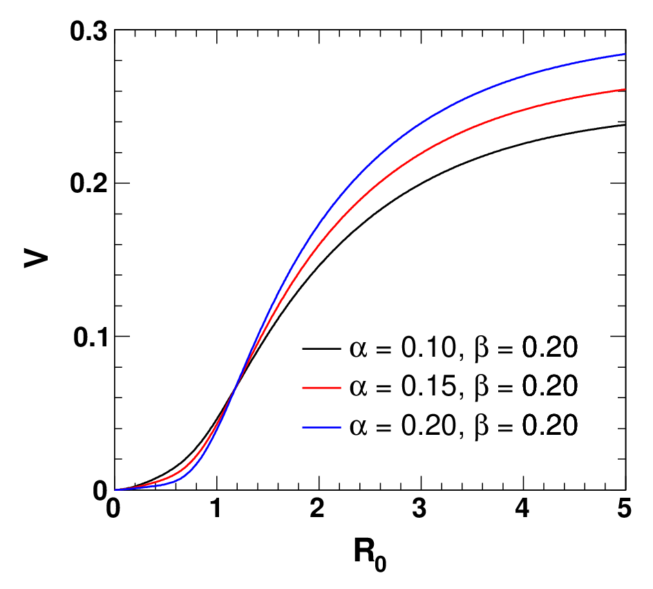
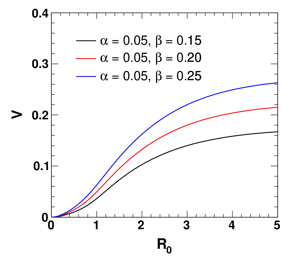
The variation of the potential with respect to for different values of and is shown in Fig. (2) in arbitrary units considering . The figure shows that the potential in Jordan frame increases gradually with respect to the background curvature with some initial deviations depending upon the values of and . In contrast to the case of mass square of the scalar field, the potential shows some slight amount of dip, but near to the same small curvature region, which increases slowly when the value of moves closer to the value of . In fact, this dip in the potential is responsible for the hump in the mass square curve for the corresponding values of and . This dip region of the potential curve almost eliminates in the case when . Moreover, with the increasing values of both and , the potential comparatively increases after the dip region or without the dip region.
II.2 Model in Einstein Frame
In order see the behaviour of our model (1) in Einstein frame, which is usually used to avoid the non - minimal coupling of gravity with the scalar field, we would like to study the model in this frame also. In the Einstein frame, the following conformal transformation of the metric is performed Goswami2013; Chakraborty2019:
which for our model takes the form:
| (25) |
Consequently, in this frame with , the action changes to Goswami2013; Chakraborty2019
| (26) |
where the scalar field
| (27) |
and is potential of the scalar field in this frame, and is given by,
| (28) |
The Eq. (27) shows the dependency of the Einstein frame scalar field on the scalar curvature . Using our model, this potential (28) can be expressed as
| (29) |
where and . Hence, the mass square term of the scalar field in the Einstein frame is
| (30) |
In Minkowski space i.e. for , this equation takes the form:
| (31) |
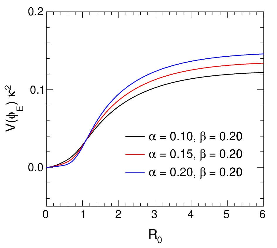
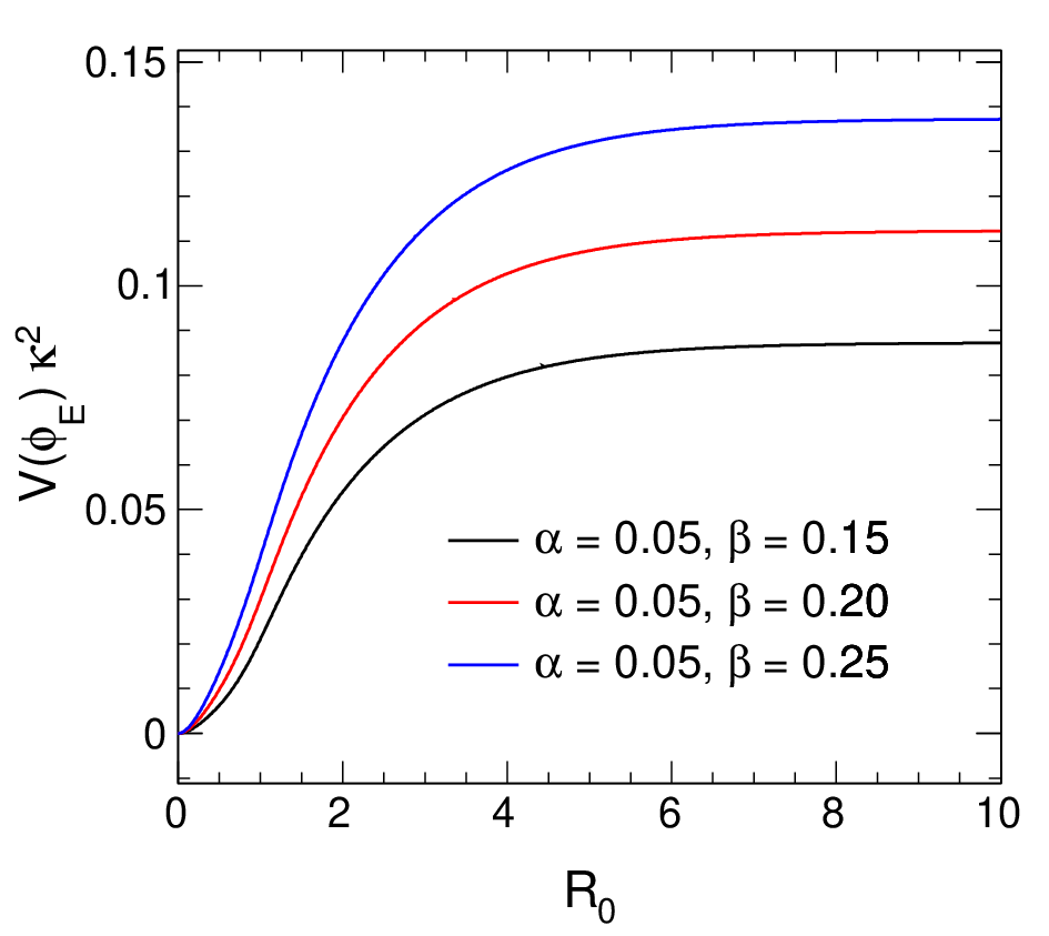


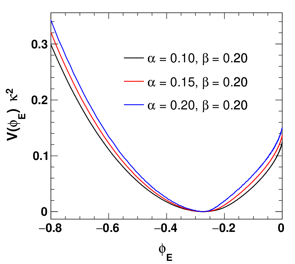
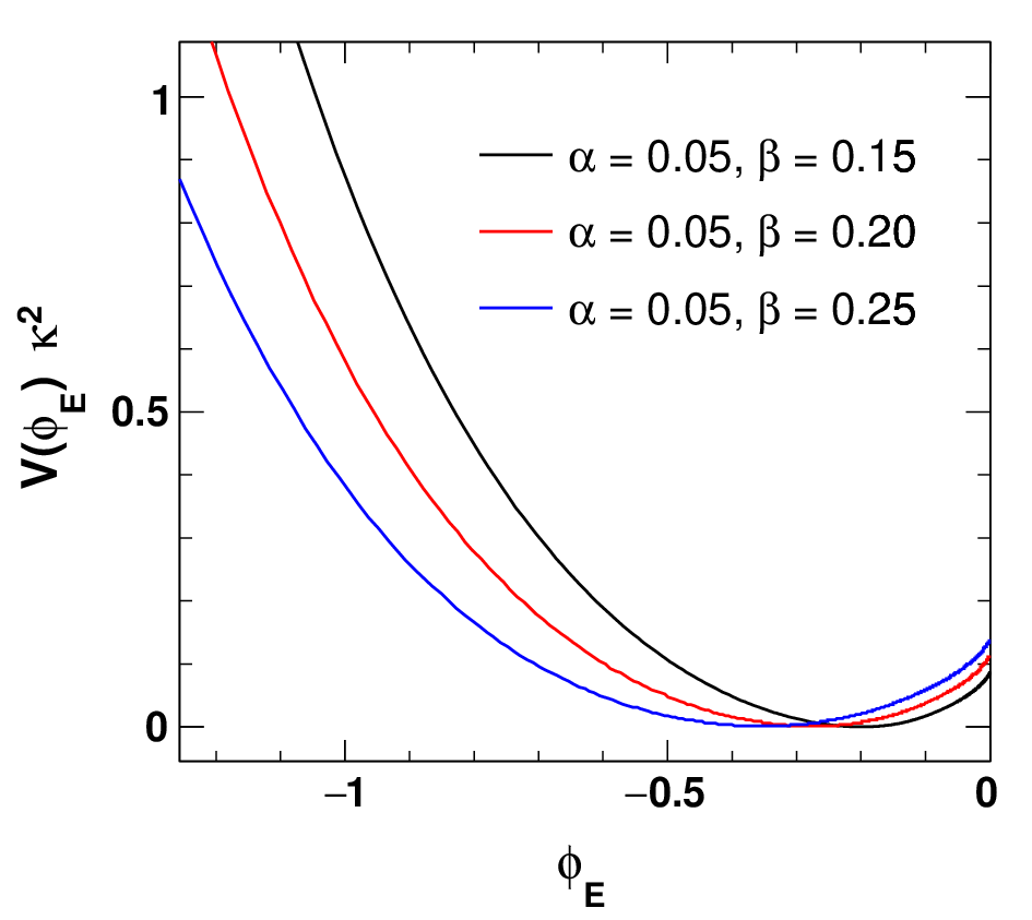
From Eq.s (29) and (II.2), we see that although the expressions for the scalar field potential and scalaron mass square in Einstein frame are little bit complicated in comparison to that in the Jordan frame, their variations as a function of are found to be almost similar as seen from Fig. 3 and Fig. 4 respectively. That is, the behaviours of potential and the mass term of the scalar field are almost identical in both frames. In Fig. 5, the variation of field as a function of background curvature is shown. The field at and is independent of , whereas it is independent of only at . Moreover, is non-zero at and tends to zero at , which is obvious from it’s expression. Again from Eq.s (11) and (27) it is clear that all these behaviours of should be applicable to also, but with positive values of for all values of . Variation of the potential (29) as a function of is shown in Fig. 6. It is seen from this figure that the minimum of the potential moves towards the higher value of when than the case when . Obviously, similar behaviour can be attributed to the potential (24) as a function of the field . Thus, because of the similarity of behaviours of the scalar field, it’s potential and mass square term in both Jordan and Einstein frames, the rest of the study in this paper is done in the Jordan frame only.
II.3 Solar System Tests of the Model
It is possible to recover GR by introducing the Chameleon mechanism in the theory. In this mechanism, the scalar field is coupled with the matter density of the environment. Thus, when a model is used inside the solar system, due to presence of matter density, the scalar field coupled with it gains mass and hence allows the model to pass the solar system tests. Clearly, this mechanism implies that the functional form should have a very closer value to the Ricci scalar , for above or equal to the solar system scale. A model is considered viable and consistent if it passes the solar system tests. Guo has introduced several methods to test whether an gravity model passes the solar system tests or not in Jordan frame Guo_2014. According to Guo, a model can pass solar system tests if it satisfies the following conditions:
| (32) |
| (33) |
| (34) |
We’ve calculated the above functions numerically for our model (see Table 1). These functions are plotted against background curvature in the units of for different parameters (see Fig. 7). These indicate that the model can be made to pass the solar system tests by increasing the ratio or by simply decreasing the parameter . However, a simple and effective way to make the model solar system viable is to decrease all the parameters (i.e. and ) sufficiently (see Table 1). Thus, within a viable range of parameters, the model can easily pass the solar system tests. This is another advantage of this model, which allows us to enlist the model as a solar system viable model.


| Values of Model parameters | |||
|---|---|---|---|
| 0.49970 | 0.49940 | 0.00060 | |
| 0.48842 | 0.47705 | 0.02235 | |
| 0.41686 | 0.34820 | 0.11727 | |
| 0.06307 | 0.04534 | 0.04534 | |
| 0.02401 | 0.01061 | 0.01657 | |
| 0.00356 | 0.00112 | 0.00226 |
III Comparison of the Model with other viable Models
In this section, we would like to compare the model with two other viable models viz., the Starobinsky model and the Hu- Sawicki model in terms of stability and nature of the models in local regime. At first, we would like study the de Sitter stability of our toy model. For our model the Eq. (2) takes the form:
where and . On solving this equation for , we get,
| (35) |
The contour plot of as a function of and is shown in Fig. 8.

The Starobinsky model and the Hu-Sawicki model are defined respectively as
| (36) |
and
| (37) |
The de Sitter solution for the Starobinsky model is
| (38) |
where . Similarly, for the Hu-Sawicki model, using the de Sitter solution is found to be,
| (39) |
The contour plots of the parameters and respectively for the Starobinsky model and the Hu-Sawicki model are shown in Fig. 9. From the contours it can be seen that for very small values of and in the Starobinsky model, we do not have de Sitter solutions. The parameter rises very rapidly for the increase of the parameters and . For the Hu-Sawicki model, we see that, there is no de Sitter solutions present for and the parameter rises very slowly for increments of beyond . On the other hand, for our toy model, we see that and have a wider region of de Sitter solutions. The other parameter has a higher value than in the de Sitter solution space towards higher values of .


The de Sitter space defined by the Eq. (35) is stable if it satisfies the condition (3). Our model (1) in Eq. (3) leads to the inequality:
| (40) |
By using Eq. (35) in the above inequality, we can further reduce it to the following form:
| (41) |
where and . When the model satisfies this Eq. (III), it can have stable de Sitter solutions. The stability region of the model in parameter space is shown in Fig.10. Again, in order to get oscillatory behaviour around the de Sitter space, the following condition needs to be satisfied motohashi:
| (42) |
Using our model in this inequality, we get,
| (43) |
Now, eliminating by using Eq. (35), we may rewrite the above expression as
| (44) |
If the toy model satisfies the above condition, it will have a stable de Sitter solution as well as oscillatory behaviour around the de Sitter solution. Similarly, for the Starobinsky model, the stability condition (3) takes the form:
| (45) |
Using Eq. (38) in the above inequality, we obtain,
| (46) |
where . The Starobinsky model gives stable de Sitter solutions for any parameter set satisfying the above inequality. For this model, the condition (42) gives,
| (47) |
Any parameter sets in the Starobinsky model satisfying this condition will give oscillations around de Sitter solutions in de Sitter space. Finally for the Hu-Sawicki model, condition (3) gives:
| (48) |
Now using Eq. (39) in the above expression and considering , we get,
| (49) |
Similarly, for the Hu-Sawicki model, the condition for existence of oscillations around stable de Sitter solutions gives:
| (50) |
We have plotted these inequalities to check the stability region of the models in parameter space in in Figs. 11 and 12.


From the Fig. 10, it is seen that the toy model has a
small region of instability
for lower values of and comparatively higher values of (greater than 0.4 approximately). For higher values of , the model has a continuous stability region in the parameter space. In case of the Starobinsky model, from
Fig. 11 it is seen that there is a small region of
instability in the parameter space. But in case of Hu-Sawicki model, the model
is stable only for the values of (Fig. 12). This suggests that, the toy model has a wider range of stability region in the parameter space. Since, the model also has a comparatively larger region admitting Eq. (42), it can be easily concluded that the toy model with a selected set of parameters can pass the stability conditions as well as the condition for having oscillatory solutions in the de Sitter space.
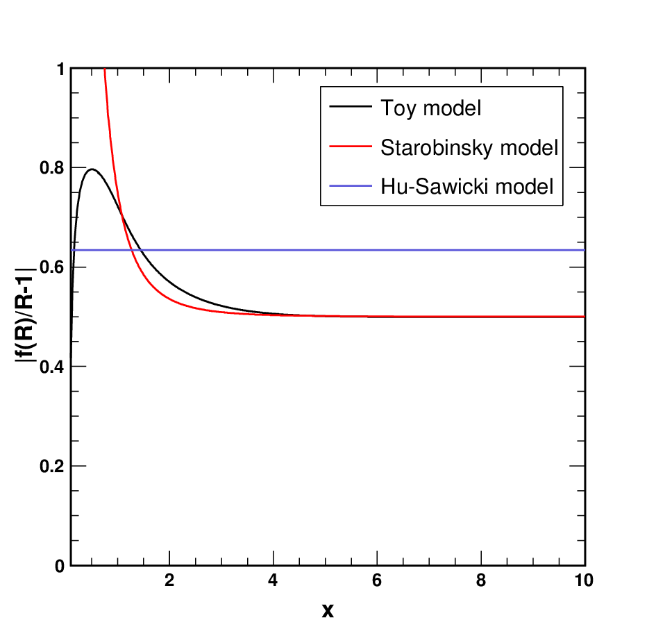
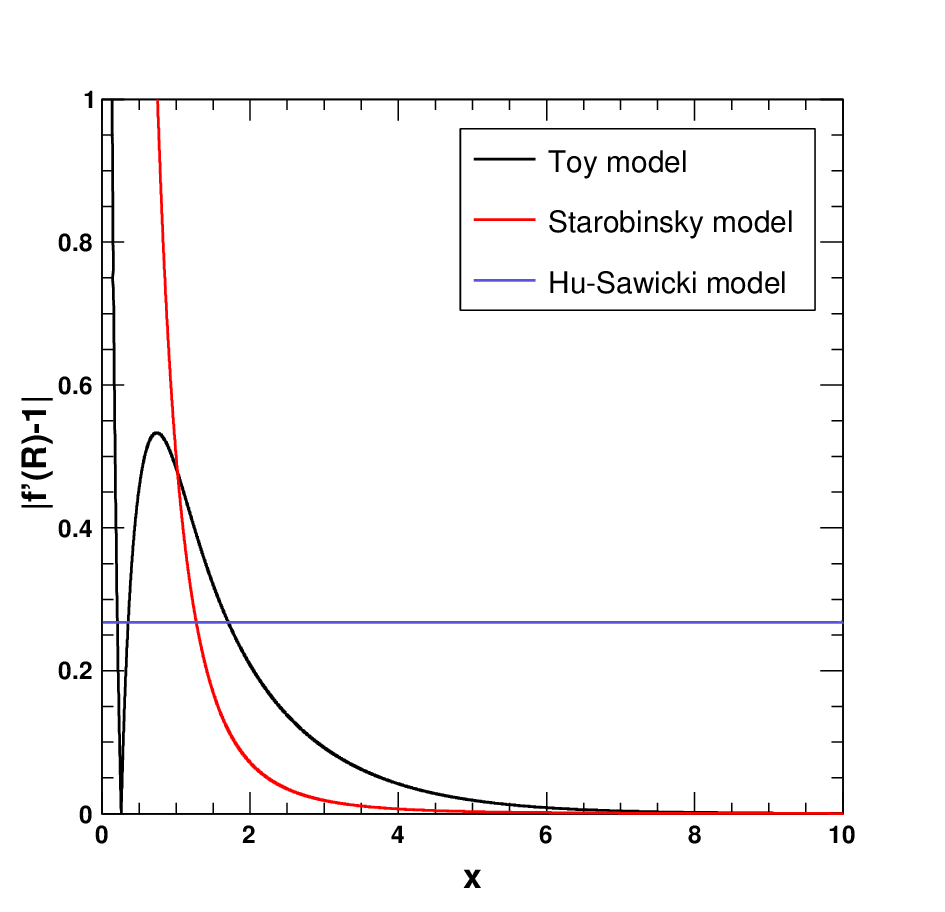
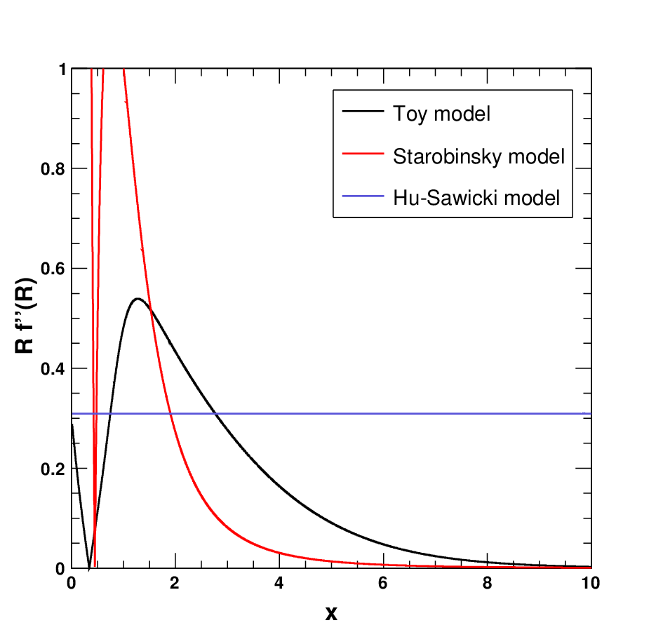
Now, we would like to compare the bahviour of the toy model with the Starobinsky and Hu-Sawicki models using the functions used in the expressions (32), (33) and (34). These expressions ensure the viability of the models in local systems. Although, in the previous section, we have chosen the parameters freely to check the solar system viabilities, now we shall study the same and compare with the other two models in de Sitter sitter stability regions of the parameter spaces. However, it should be noted that most of the parameter sets used in that sections are found to belong automatically in the de Sitter sitter stability region of the model. The function used in relation (32) takes the following respective form in the toy model, Starobinsky model and Hu-Sawicki model in the de Sitter solution regime,
| (51) |
| (55) |
and
| (56) |
The third function for the respective models are calculated as:
| (57) |
| (58) |
and
| (59) |
These functions for the said models are compared in Fig. 13. It is seen that the models are capable of passing the solar system tests in the de Sitter stable regime for higher values of . The Hu-Sawicki model in this regime shows a constant behaviour. However, the Starobinsky model and the toy model give the higher values of the test functions for lower values. In this case, the behaviour of the toy model still indicates the ability to pass the solar system tests. One interesting point to note that for the toy model and the Starobinsky model, the asymptotic behaviours of the test functions are almost same. These results suggest that the behaviour of the toy model is closer to the Starobinsky model. However, to make a clear conclusion, a detailed study of the models is required and this is beyond the scope of this manuscript.


IV Constraints on the Model
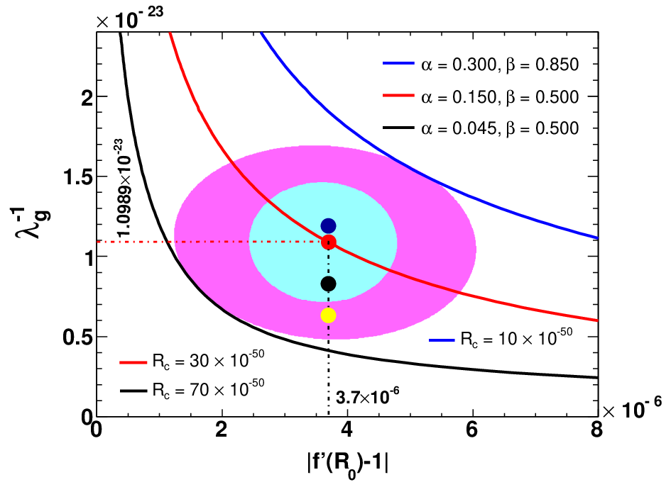
For the viability of a model in gravity it is utmost necessary to impose constraints on the model on the basis of different available observational data. A model which passes such constraints are considered as a viable model in gravity. Starobinsky model and Hu Sawicki model are examples of two viable models in this context as mentioned earlier. There are several ways to constrain an gravity model Boubekeur_2014; Desai_2018; Jana_2019; Gupta_2019; Chiba_2007; Cataneo_2015; Nunes_2017. A constrained model is helpful to study different implications of the model. In this section, we will try to constrain our toy model using the results published in Boubekeur_2014; Desai_2018 and Jana_2019. In Ref. Boubekeur_2014, authors carried out a Markov chain Monte Carlo (MCMC) analysis for GWs from Hu Sawicki model using the data sets of cosmic microwave background (CMB) and baryon acoustic oscillations (BAO) together with the independent constraints on the relationship between the matter clustering amplitude and the matter mass-energy density from Planck Sunyaev-Zeldovich (PSZ) cluster number counts and also from the CFHTLens weak lensing tomography measurements. Combining CMB, BAO and relationship from the PSZ catalog Ade_2014, they obtained a bound which is still better than the bounds obtained from the GW event GW170817 Jana_2019. The bound on the parameter reported by them is
| (60) |
with confidence level at upper bound Boubekeur_2014. On the other hand in Ref. Desai_2018 a constraint was introduced on the Compton wavelength of the graviton. From their study, we have a constraint on as given by,
| (61) |
with confidence level on upper bound Desai_2018.
Now, we have computed the values of and for our model by taking into consideration of above cited respective upper bounds with the corresponding confidence levels to constraint our model parameters and . The results of this computation along with the contour plots are shown in Fig. 14. Here we have not considered the constraint on the model parameters coming from the fact that at higher curvatures it goes near to the cosmological constant. However, the parameters are chosen from the stability region of the parameter space. It is seen that the model can be a viable one within a proper range of variables. The figure shows the contours with confidence level for and confidence level for (the larger contour) and with confidence level for the both (the smaller contour). The central point denotes the boundary value for both the parameters and and any value lower than the boundary value is viable. This point corresponds to the galaxy cluster Abell 1689 data Desai_2018. In the plots we have considered three sets of the parameters and we see that the smaller values of allow the model to pass the constraints easily. In the Fig. 14, we have also shown 3 other points corresponding to galaxy clusters Abell 262, Abell 1991 and Abell 383 data from the Ref. Gupta_2019. All these points lie within the confidence level contours.
The model can be constrained by using the GWs event GW170817 also. In a recent study Jana_2019, gravity was constrained by using the GW170817. They provided a bound on , which is
| (62) |
Using our toy model in this expression, we find,
| (63) |
Now, using Eq. (35) in the above expression, we can have,
| (64) |
Choosing (an arbitrary point in the stability region from Fig. 10) and considering to be a positive quantity, the above equation reduces to,
| (65) |


.
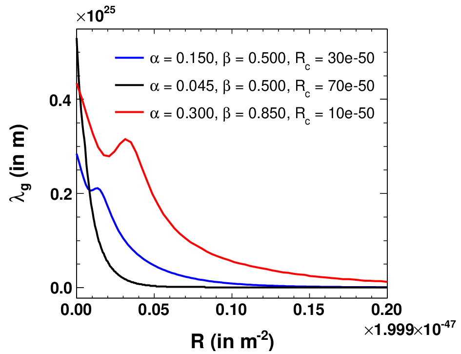
In Fig. 15, we have shown the variations of with respect to , with respect to and with respect to for the values of the model parameters used in the contour plots in Fig. 14. The hump in the mass of the scalar field encountered in the Fig. 1 and in the Fig. 6 are also present in the vs. curves. However, as mentioned earlier, this hump vanishes when . For higher curvatures, rapidly moves towards zero. The function also has significantly higher values near the Minkowski spacetime and as soon as the background Ricci curvature increases, this model dependent function decreases rapidly. This nature of the model is suitable for overcoming the local system constraints. Again as seen from the figure, with the increase of the function mass of the scalar field decreases initially at a faster rate and then becomes almost constant at later stage.
V Polarization Modes of GWs in the Model
In this section, we wish to check the polarization modes of GWs in the model. In presence of massive polarization mode, it would be easy to constraint the model using the experimental results. To explore the polarization modes of GWs in the model, at first we’ll introduce the perturbation to the field equation.
V.1 Perturbation to the Field Equation
If there are propagating GWs in spacetime, then they perturbs the metric around its background value. Considering the background metric as we may express the spacetime metric to the first order of perturbation value , which is usually usually very small, as
| (66) |
Now, expanding the Ricci tensor and the Ricci scalar upto the first order of , we may write:
| (67) |
and
| (68) |
Similarly, we may write for the and as
| (69) | ||||
| (70) |
where is some constant curvature. Thus, due to the perturbation in spacetime the trace equation (9) can be rewritten as
| (71) |
where we have used for the empty space or far away from the source. Fixing the gauge to be harmonic gauge with , which after operating by we find,
| (72) |
An important point to be mentioned here is that, the Eq. (8) is also satisfied by another solution: , giving
| (73) |
This equation actually corresponds to the Eq. (15), which is the stationary condition used earlier in the Sec. II. In empty space, this equation has the form:
| (74) |
and it leads to have the equation,
| (75) |
This is the stationary condition (15) of the scalar field potential in the empty space corresponding to the constant curvature of spacetime. Using the Eq.s (68), (72) and (75) in Eq. (71), we get
| (76) |
Now, we would like to define , where is the mass of the associated scalar field. Using this definition in the above equation we obtain,
| (77) |
This is a quadratic equation in and solution for gives,
| (78) |
and
| (79) |
We see that the second solution corresponds to tachyonic scalar field which becomes zero in the Minkowski spacetime or at far distance away from the source. The first solution is identical to Eq. (16). Thus the term given by Eq. (78) is exactly same as the scalar field mass square term given in Eq. (17) for our model, when . Therefore this solution suggests that there exists a massive scalar mode of polarization of GWs in the theory apart from the massless tensor modes.
At very far distance away from the source, we can consider , i.e. the Minkowski metric and the background curvature . In this case, the Ricci scalar slowly varies near zero, i.e. . Hence, for the Minkowski space the Eq. (66) can be written as
| (80) |
And to the first order of , we get
| (81) |
| (82) |
where . So for our model, to the first order of perturbation, the Eq. (8) becomes
| (83) |
Taking the trace of this Eq. (83), we get
| (84) |
where
with and . This is also exactly the same mass square term in Minkowski space given by the Eq. (18) for our model. Next, we introduce a variable
| (85) |
The trace of this variable is
| (86) |
Using this Eq. (86) in the variable (85) we find,
| (87) |
From Eq. (85) and Eq. (87), one can easily see that both and are interchangeable, i.e. replacing by and vice-versa in Eq. (85) gives Eq. (87). Again, under an infinitesimal coordinate transformation, , we have
| (88) |
The trace of this equation is
| (89) |
And
| (90) |
The trace trace of this equation gives,
| (91) |
Here we raise or lower the indices with the help of , i.e. with the Minkowski metric. The Lorentz gauge condition can be obtained if satisfies . The Lorentz gauge condition does not constrain the gauge freedom and there is always a possibility to choose the transverse and traceless conditions, i.e. and Liang_2017; Corda_2007; Corda_2008; Capozziello_2008. By using the transverse traceless gauge condition and substituting the Eq. (87) into Eq. (81), we get
| (92) |
Plugging Eq. (92) into Eq. (83), we obtain
| (93) |
Combining Eq.s (84) and (93), we get
| (94) |
which is the wave equation of the massless tensor field. The solution to this Eq. (94) is Corda_2007; Corda_2008
| (95) |
where and . Whereas the solution to the massive scalar field Eq. (84) is given by Corda_2007; Corda_2008,
| (96) |
where . Assuming the GWs propagation direction along , the general solution can be written as Liang_2017
| (97) |
where is transverse and traceless and it represents the standard spin-2 graviton, and represents the scalar field which is massive in nature and travels with a speed less than . The solution of the scalar part along axis, i.e. can be expressed as
| (98) |
and hence the mass of the field in terms of and is
| (99) |
V.2 Calculation of Exact Polarization amplitudes and Newman-Penrose Quantities of the Model
In 1973, a powerful method was introduced in Ref. Eardley_1973 which deals with the study of the properties of GWs in any metric theory of gravity. This method involves analysing all the relevant components of Riemann tensor, which results relative acceleration between two test particles. They used a null-tetrad basis in order to calculate the Newman-Penrose quantities Newman_1962. In the Newman-Penrose formalism, there are ten ’s, nine ’s, and a , which are algebraically independent and represent the irreducible parts of the Riemann tensor . They are known as Newman-Penrose quantities. But in case of plane waves or nearly plane waves, the differential and symmetry properties of reduce the number of independent, nonvanishing components, to six. Hence, in this formalism, the set is used to describe the six independent components of GWs in the metric theory. In the tetrad basis, the Newman-Penrose quantities of the Riemann tensor are Eardley_1973:
| (100) | ||||
| (101) | ||||
| (102) | ||||
| (103) |
It should be noted that, and are complex. Therefore, each one of them is capable of describing two independent polarizations. One polarization mode for the real part and one for the imaginary part. Thus total number of polarization modes is 6.
The tetrad components of Ricci tensors can be expressed as Eardley_1973,
| (104) | ||||
| (105) | ||||
| (106) | ||||
| (107) |
and the Ricci scalar is
| (108) |
In normal coordinate system Eardley_1973,
Although the amplitudes of a wave depend on the observer Eardley_1973, there are certain invariant statements about them that hold true for all the standard observers if they hold true for any one. These statements characterize the invariant classes of waves. For a standard observer, under the assumptions that (a) the wave travels in the direction, and (b) the same frequency for a monochromatic wave is observed, the classes are:
- •
Class : . Standard observers measure the same non-vanishing amplitude in the mode. Presence or absence of all other modes is observer-dependent;
- •
Class : . Standard observers measure the absence of and the presence of . Presence or absence of and is observer-dependent;
- •
Class : . Presence or absence of all modes is observer-independent;
- •
Class : . Observer-independent;
- •
Class : . Observer-independent;
- •
Class : . Observer-independent. All standard observers measure no wave.
In gravity, the field equation derived from the Lagrangian in metric formalism results dynamical expressions for Ricci tensor and Ricci scalar, as we have already seen. Using this method, the expressions for Ricci tensor and scalar are calculated in weak field limit, i.e. far from the GWs source considering that the GW is propagating along axis. Thus, the Ricci tensor components corresponding to directions other than and will vanish. But from earlier sections, we see that a massive scalar mode of polarization is present in this model and so it is not possible to use this Newman-Penrose formalism formalism which is developed for null waves Liang_2017. For waves with massive propagation mode, modified Newman-Penrose formalism has to be applied Hyun_2019. In modified Newman-Penrose formalism, the polarization amplitudes as well as Newman-Penrose quantities are calculated for a massive wave subject to proper gauge condition. Considering the monochromatic wave solution of the form:
| (109) |
where is the frequency and is the wave number. However, we have noticed that, the modified Newman-Penrose scalars and polarization amplitudes introduced in Hyun_2019 using Lorentz gauge condition can not distinguish breathing mode when the scalar field becomes massless. It is due to the fact that, they have used the transverse traceless condition to make the non-tensor modes vanish when . But can’t demand because, the breathing mode is massless in nature Gogoi_2019. Breathing modes satisfy the transverse condition but not the traceless condition. It implies that a model having can have massless breathing mode of polarization Gogoi_2019. Keeping this fact in mind, we have modified the polarization amplitudes and Newman-Penrose quantities. According to our calculations, modified polarization amplitudes are expressed as:
| (110) |
Here, we have not applied the traceless condition to the breathing mode. These are the exact polarization amplitudes of the wave. These expressions are valid for any metric theory. The modified Newman-Penrose quantities now can be expressed as:
| (111) |
These equations differ from those in Ref. Hyun_2019.
Now, for our model the general wave solution is given by Eq. (97). Using this Eq. (97) in the above set of Eq.s (110), we found the polarization amplitudes for our model as
| (112) |
where is given by Eq. (99) and (see Eq. (97)). From the above expressions we can calculate the Newman-Penrose quantities. Note that, above results suggest, there are non-zero polarization amplitudes in the theory. Using Eq.s (111), we’ve calculated the Newman-Penrose quantities for the model as
| (113) |
Thus the classification of the model is . The model exhibits non-zero Newman-Penrose quantities for polarization modes viz., tensor plus, tensor cross, scalar transverse massless breathing mode and scalar longitudinal massive mode of polarization. However, the degrees of freedom associated with the theory is . This suggests that the breathing mode and the longitudinal mode exist in a mixed state to give rise to a single polarization mode. If , the massive longitudinal mode will vanish, giving . Note that is not a sufficient condition to imply the absence of scalar degrees of freedom in the theory. It is because, in theory there exists massless breathing mode which is transverse but not traceless. Absence of scalar degrees of freedom requires both and . When both and vanish, the theory reduces to GR giving only tensor modes of polarizations.
VI Detection of Polarization Modes of GWs - A Review
Experimental detection of polarization modes of GWs is very important to know the exact nature of GWs and hence in checking the viabilities of modified gravity theories. In this section we discuss the Pulsar Timing Arrays (PTAs) as a tool to distinguish between different polarization modes. Moreover, we include a discussion on the results based on our model.
PTAs play a significant role in the indirect detection of GWs. They are also used for numerous astrophysical applications. In 1968, Counselman & Shapiro explained that the observations of pulsars could be used to test GR Counselman_1968. Later in 1982, the first millisecond pulsar was discovered Backer_1982. Till now, a pretty good number of millisecond pulsars has been discovered. The advantage of these pulsars over the normal pulsars is that they are very stable. Their arrival times can be measured and predicted with a good accuracy. This allows to use these pulsars as a probe to search for GWs. In 2004, the Parkes Pulsar Timing Array (PPTA) project began with the Parkes 64 m telescope Manchester2013; Oslowski2019. After three years, the North American Nanohertz Observatory for Gravitational Waves (NANOGrav) in North America was founded Brazier2019; Arzoumanian2016. NANOGrav uses the Arecibo and Green Bank telescopes to observe around 36 pulsars. In the same year, the European Pulsar Timing Array (EPTA) project was also founded Desvignes2016. Using the Sardinian, Effelsberg, Nancay, Westerbork and Jodrell Bank telescopes, EPTA observes around 42 pulsars. Later, by combining these three projects, the International Pulsar Timing Array (IPTA) was formed Verbiest2016; Perera2019. In this study, we have used some selected data from PPTA Manchester2013 and IPTA Verbiest2016; Perera2019.


From the Ref. Lee_2008, we can have the correlation functions for different polarization modes. The calculation of correlation functions for the tensor and breathing modes are model independent, but in the case of massive longitudinal mode, the correlation function is model dependent as it depends on the mass of the scaler graviton. The correlation function for tensor modes is Lee_2008
| (114) |
where
and is the angular separation between two pulsars. For the scalar modes it is Lee_2008
| (115) |
where
The normalized correlation function in general is given by:
These are the correlation functions for tensor modes and massless breathing mode of GW polarization. But in our model, there exists a massive longitudinal mode. Thus to see the effect of massive mode, we follow the Refs. Jenet_2005; Lee_2013; Lee_2010 in which the timing residual induced by GWs is expressed as
| (116) |
here gives the dispersion relation of the GWs, the terms and connect the mass of the longitudinal mode of polarization by the relation , and . is the displacement vector from the observer to the pulsar and and are two unit vectors pointing to two pulsars. The correlation coefficient between two different pulsars is given by
where the sub-scripts are indices for the pulsars. With these assumptions and following Ref. Lee_2008, the correlation functions are calculated numerically for different values of (see Fig. 16). In terms of our model,
All these numerically calculated correlation functions are plotted with respect
to in Fig. 16. In this figure we have used three values
of for the following sets of parameters:
(i) for ,
(ii) eV for and
(iii) eV for
To check the experimental viability of our model, we have calculated the correlation functions for GWs using some selected data from IPTA and PPTA data set Manchester2013; Verbiest2016; Perera2019; Hobbs2006; Edwards2006 as mentioned above, which are also plotted in Fig. 16. Although we do not have a clear conclusion, which requires more observation period as well as data, we can still see that these experimental data could not directly rule out the existence of extra polarization modes of GWs. However, to distinguish between polarization modes, we need to wait for more PTA data with GW events.
VII Summary and Conclusion
In this work, we have introduced a new gravity toy model and studied the polarization modes of GWs in it. The study shows that, in metric formalism, there exists polarization modes of GWs viz., tensor plus mode, tensor cross mode and scalar mode. The scalar mode is a mixed state of massless breathing mode and massive longitudinal mode. The tensor modes of polarization are transverse, traceless and massless in nature. The scalar breathing mode is transverse but exists with non vanishing trace and massless in nature. On the other hand, the scalar longitudinal mode is massive in nature and hence propagates with speed less than that of tensor modes. When the scalar field becomes massless, the longitudinal mode vanishes and only the massless scalar breathing mode exists in the scalar degrees of freedom. As an experimental correspondence of our model prediction on the modes of GWs, we have compared the correlation function of massive longitudinal mode as predicted by the model with that of the some selected PTAs data of PPTA and IPTA. The result is found to be quite encouraging.
We have also shown that a wisely selected set of the parameters easily allows the model to pass the solar system tests, which is a very important requirement for the viability of a model. Further, the model has been constrained using combined CMB, BAO and relationship from the PSZ catalog and Abell 1689 galaxy cluster data. The model can be easily constrained with the help of the parameters , and . Further, we have also constrained the model using the GW event GW170817. It is seen that, the model can withstand the constraints put by GW170817 and hence can be included as a post GW170817 viable model.
In the present work, we have studied only few properties of the model. However, for a proper understanding of the model characteristics, a detailed study is required. As such, in future the model can be checked also for various stabilities and constraints as well as in different cosmological and astrophysical contexts, which will give us more information about the viability of the model. Moreover, it is to be noted that in the Palatini formalism the polarization modes of GWs in gravity is model independent. So, this formalism can not distinguish our model from other gravity models in this context. Nevertheless, there may be some cosmological variations and stellar structure differences of the model in Palatini formalism, which might be useful to study the generation of GWs in such situations.
Acknowledgement
A part of this work was done during a visit of authors to IUCAA, Pune. Authors are grateful to IUCAA for the hospitality during their stay.
References
- (1) A. G. Riess et al., Astron. J. 116, 1009 (1998).
- (2) S. Perlmutter et al., Astrophys. J. 517, 565 (1999).
- (3) N. A. Bahcall, J. P. Ostriker, S. Perlmutter and P. J. Steinhardt, Science 284, 1481 (1999) [arXiv:astro-ph/9906463].
- (4) R. P. Kirshner, PNAS 96, 4224 (1999).
- (5) C. Corda, Int. J. Mod. Phys. A 23 (10), 1521 (2008).
- (6) B. P. Abbott et al., Phys. Rev. Lett. 116, 061102 (2016).
- (7) A. A. Starobinsky, JETP Lett. 86, 157 (2007) [arXiv:0706.2041].
- (8) W. Hu and I. Sawicki, Phys. Rev. D 76, 064004 (2007) [arXiv:0705.1158].
- (9) S. Tsujikawa, Phys. Rev. D 77, 023507 (2008) [arXiv:0709.1391].
- (10) P. Zhang, Phys. Rev. D 73, 123504 (2006) [arXiv:astro-ph/0511218].
- (11) G. Cognola et al., Phys. Rev. D 77, 046009 (2008) [arXiv:0712.4017].
- (12) E.V. Linder, Phys. Rev. D 80, 123528 (2009) [arXiv:0905.2962].
- (13) C. Corda, JCAP 04, 009 (2007).
- (14) D. Liang, Y. Gong, S. Hou and Y. Liu, Phys. Rev. D 95, 104034 (2017).
- (15) D. J. Gogoi and U. D. Goswami, arXiv:1901.11277 (2019).
- (16) Y.-C. Chen, C.-Q. Geng, C.-C. Lee, and H. Yu, Eur. Phys. J. C 79, 93 (2019).
- (17) L. Amendola, S. Tsujikawa, Dark Energy: Theory and Observations (Cambridge University Press, Cambridge, 2015).
- (18) L. Amendola, R. Gannouji, D. Polarski, and S. Tsujikawa, Phys. Rev. D 75, 083504 (2007) [arXiv:gr-qc/0612180].
- (19) K. Bamba, C.Q. Geng and C.C. Lee, JCAP 1011, 001 (2010) [arXiv:1007.0482].
- (20) H. Motohashi, A. A. Starobinsky, and J. Yokoyama, JCAP 06, 006 (2011) [arXiv:1101.0744].
- (21) S. Capozziello, A. Stabile and A. Troisi, Class. Quantum Grav. 24, 2153 (2007) [arXiv:gr-qc/0703067].
- (22) P. Teyssandier and P. Tourrenc, J. Math. Phys. (N.Y.) 24, 2793 (1983).
- (23) U. D. Goswami and K. Deka, Int. J. Mod. Phys. D 22, 1350083 (2013) [arXiv:1303.5868].
- (24) S. Chakraborty, S. Pal, and A. Saa, Phys. Rev. D 99, 024020 (2019) [arXiv:1812.01694].
- (25) J.-Q. Guo, Int. J. Mod. Phys. D 23, 1450036 (2014) [arXiv:1306.1853].
- (26) L. Boubekeur et al., Phys. Rev. D 90, 103512 (2014).
- (27) S. Desai, Phys. Lett. B 778, 325 (2018) [arXiv:1708.06502].
- (28) S. Gupta and S. Desai, Class. Quantum Grav. 36, 105001 (2019) [arXiv:1811.09378].
- (29) S. Jana and S. Mohanty, Phys. Rev. D 99, 044056 (2019) [arXiv:1807.04060].
- (30) T. Chiba, T. L. Smith, and A. L. Erickcek, Phys. Rev. D 75, 124014 (2007).
- (31) M. Cataneo et al., Phys. Rev. D 92, 044009 (2015) [arXiv:1412.0133].
- (32) R. C. Nunes, S. Pan, E. N. Saridakis, and E. M. C. Abreu, J. Cosmol. Astropart. Phys. 01, 005 (2017).
- (33) P. A. R. Ade et al. (Planck Collaboration), AA 571, A20 (2014) [arXiv:1303.5080].
- (34) C. Corda, J. Cosmol. Astropart. Phys. 04, 009 (2007).
- (35) C. Corda, Int. J. Mod. Phys. A23, 1521 (2008).
- (36) S. Capozziello, C. Corda, and M. F. De Laurentis, Phys. Lett. B 669, 255 (2008).
- (37) D. M. Eardley, D.L. Lee, A.P. Lightman, Phys. Rev. D 8, 3308 (1973).
- (38) E. Newman, R. Penrose, J. Math. Phys. 3, 566 (1962).
- (39) Y.-H. Hyun, Y. Kim, and S. Lee, Phys. Rev. D 99, 124002 (2019).
- (40) C. C. Counselman III and Shapiro II, Science 162, 352 (1968).
- (41) D. C. Backer, S. R. Kulkarni and C. Heiles et al., Nature 300, 615 (1982).
- (42) R. N. Manchester et al., Publ. Astron. Soc. Aust. 30, e017 (2013) [arXiv:1210.6130].
- (43) S. Osłowski et al., Mon. Not. R. Astron. Soc. 488, 868 (2019) [arXiv:1906.09793].
- (44) A. Brazier et al., arXiv:1908.05356 (2019).
- (45) Z. Arzoumanian et al., ApJ 821, 13 (2016) [arXiv:1508.03024].
- (46) G. Desvignes et al., Mon. Not. R. Astron. Soc. 458, 3341 (2016) [arXiv:1602.08511].
- (47) J. P. W. Verbiest et al., Mon. Not. R. Astron. Soc. 458, 1267 (2016) [arXiv:1602.03640].
- (48) B. B. P. Perera et al., Mon. Not. R. Astron. Soc. 490, 4666 (2019) [arXiv:1909.04534].
- (49) K. J. Lee, F. A. Jenet, and R. H. Price, ApJ 685, 1304 (2008).
- (50) F. A. Jenet, G. B. Hobbs, K. J. Lee, and R. N. Manchester, ApJ 625, L123 (2005).
- (51) K. J. Lee, Class. Quantum Grav. 30, 224016 (2013) [arXiv:1404.2090].
- (52) K. Lee, F. A. Jenet, R. H. Price, N. Wex, and M. Kramer, ApJ 722, 1589 (2010) [arXiv:1008.2561].
- (53) G. B. Hobbs, R. T. Edwards, and R. N. Manchester, Mon. Not. R. Astron. Soc. 369, 655 (2006) [arXiv:astro-ph/0603381].
- (54) R. T. Edwards, G. B. Hobbs, and R. N. Manchester, Mon. Not. R. Astron. Soc. 372, 1549 (2006) [arXiv:astro-ph/0607664].