A comprehensive power spectral density analysis of astronomical time series I:
the Fermi-LAT gamma-ray light curves of selected blazarsMathematica (Wolfram Research 2016), R (R Core Team 2016, http://www.R-project.org), carma_pack (Kelly et al. 2014, https://github.com/bckelly80/carma_pack), wavepal (Lenoir & Crucifix 2018a; Lenoir & Crucifix 2018b, https://github.com/guillaumelenoir/WAVEPAL), Matlab (MATLAB 2010)
Abstract
We present the results of the Fermi-LAT 10-years-long light curves (LCs) modeling of selected blazars: six flat spectrum radio quasars (FSRQs) and five BL Lacertae (BL Lacs), examined in 7-, 10-, and 14-day binning. The LCs and power spectral densities (PSDs) were investigated with various methods: Fourier transform, Lomb-Scargle periodogram (LSP), wavelet scalogram, autoregressive moving average (ARMA) process, continuous-time ARMA (CARMA), Hurst exponent (), and the plane. First, with extensive simulations we showed that parametric modeling returns unreliable parameters, with a high dispersion for different realizations of the same stochastic model. Hence any such analysis should be supported with Monte Carlo simulations. For our blazar sample, we find that the power law indices calculated from the Fourier and LSP modeling mostly fall in the range . Using the wavelet scalograms, we confirm a quasi-periodic oscillation (QPO) in PKS 2155304 at a significance level, but do not detect any QPOs in other objects. The ARMA fits reached higher orders for 7-day binned LCs and lower orders for 10- and 14-days binned LCs for the majority of blazars, suggesting there might exist a characteristic timescale for the perturbations in the jet and/or accretion disk to die out. ARMA and CARMA modeling revealed breaks in their PSDs at timescales of few hundred days. The estimation of was performed with several methods. We find that most blazars exhibit , indicating long-term memory. Finally, the FSRQ and BL Lac subclasses are clearly separated in the plane.
Keywords:
galaxies: active — quasars: general — BL Lacertae objects: general — galaxies: jets — gamma rays: galaxies — methods: statistical — BL Lacertae objects: individual (TXS 0506+056) — quasars: individual (PKS 1830211)I Introduction
Blazars are jetted radio-loud objects, which constitute a peculiar class of active galactic nuclei (AGNs). They are originally defined as extragalactic objects which possess a non-thermal continuum along the entire electromagnetic spectrum, exhibit high degree of radio-to-optical polarization, compact radio emission, and pointing their relativistic jets towards an observer (see e.g., Angel & Stockman 1980; Urry & Padovani 1995; Padovani et al. 2017, for a review). Blazars show variability in different energy bands, often rapid with shortly lasting flares, from months down to minutes (Wagner & Witzel 1995; Rani et al. 2010b; Nilsson et al. 2018). They are commonly divided into two subgroups, i.e. flat spectrum radio quasars (FSRQs) and BL Lacertae (BL Lac) objects, based on characteristics visible in their optical spectra. FSRQs have prominent emission lines with the equivalent width 5 Å, while spectra of BL Lacs are featureless (with a smooth continuum) or display weak lines only. This division can be also done based on different accretion regimes of AGNs, i.e. FSRQs have high accretion rates, while BL Lacs have low accretion rates (Ghisellini et al. 2011). Moreover, taking into account the position of the synchrotron peak, , of the spectral energy distribution (SED; in the plane), BL Lacs are split into low-peaked (LBL), intermediate-peaked (IBL), and high-peaked (HBL) BL Lacs (Abdo et al. 2010c). An additional group of extreme HBL, having is also considered (Costamante et al. 2001; Akiyama et al. 2016).
Over the years, many multiwavelength as well as different single energy band studies have been conducted to investigate the physical processes causing variability visible in blazars’ light curves (LCs), especially their power spectral densities (PSDs). In particular, the timescales at which the PSD changes its character, e.g. breaks, could give an indication of the emission regions, i.e. accretion disk in for instance FSRQs, miscoquasars, or X-ray binary systems, or jet in BL Lacs, and thus of the physical mechanism of observed variations caused in these regions. Several LC investigations were based on the high energy (HE; ) -ray Fermi-Large Area Telescope (LAT) data. 11-months-long weekly-binned LCs of 104 blazars, including 58 FSRQs, 42 BL Lacs, and four objects with uncertain classification, were analyzed by Abdo et al. 2010b. Their PSDs were obtained with the structure function (SF) and fitted with a power law (PL), , giving an index for a majority of blazars. It was also found that the FSRQs, LBLs, and IBLs show larger variations than HBLs, wherein all studied blazars can be described as steady sources with a series of flares. Sobolewska et al. 2014 studied 4-years-long, adaptively-binned, densely-sampled Fermi-LAT LCs of 13 well known and bright blazars, i.e. eight FSRQs and five BL Lacs. The LCs were modeled with the Ornstein–Uhlenbeck (OU) process, and a superposition of OU processes (sup-OU). It turned out that the majority (i.e., 10) of investigated objects are better described by the sup-OU model, with the PL index 1. It is worth mentioning that the index does not depend on the redshift or blazar classification. Recently, Ryan et al. 2019 analyzed long-term (9.5 years) daily- and weekly-binned Fermi-LAT LCs (taken from the Fermi Science Support Center11 1 http://fermi.gsfc.nasa.gov/ssc/data/access/lat/msl_lc/) of 13 blazars previously studied by Sobolewska et al. 2014. The LCs were analyzed with the continuous-time autoregressive moving average (CARMA) model (Kelly et al. 2014), indicating that the OU processes, i.e. CARMA(1,0), do not pick up the characteristics of variability in the data, while higher-order processes, i.e. CARMA(2,1), provide a much better description of the variability. The multiwavelength analysis of the famous source OJ 287 yielded CARMA as the best fit for the HE data, while optical and radio LCs (with much more measurements) exhibited higher-order CARMA models (Goyal et al. 2018).
Regarding the PSD study, quasi-periodic oscillations (QPOs) in AGN, where a QPO is defined as ”concentration of variability power over a limited frequency range” (Vaughan & Uttley 2005), may help to establish the variability regions and physical processes responsible for variability as well as to place constraints on the black hole (BH) mass estimations as it is in the case of microquasars, neutron stars, and X-ray sources (Stella & Vietri 1998; Muno et al. 1999; Abramowicz et al. 2004; Török et al. 2005, e.g.). Most of the analyses aimed at searching for QPOs focus around different implementations of periodograms and scalograms. Espaillat et al. 2008 analyzed X-ray XMM-Newton LCs of 10 bright AGNs. The observations were conducted in the energy range keV, while the analysis was performed with the continuous wavelet transform and the SF. A QPO was found for only one AGN, i.e. 3C 273, with a period of 55 minutes at the significance level , and a range of BH mass was estimated as , . Lachowicz et al. 2009 looked for QPOs in the keV band observations of PKS 2155304 by analyzing a 64 ks XMM-Newton LC with the multi-harmonic analysis of variance periodogram (Schwarzenberg-Czerny 1996), the SF, and the wavelet scalogram (Torrence & Compo 1998). A QPO with a period of h was found in the data at significance level, which allowed authors to estimate the BH mass to be within the range , . Gupta et al. 2009 collected a set of 20 V and R filter optical LCs of the blazar PKS 0716+714, lasting from 7.7 h up to 12.3 h. Each LC was studied separately with a wavelet plus randomization technique, giving a set of possible QPO timescales and corresponding BH mass estimates (see Table 1 in Gupta et al. 2009 for details). Subsequently, Rani et al. 2010a studied a 9.6-hour-long R-band optical LC of PKS 0716+714, delivered by the Physical Research Laboratory in India, using the SF analysis, Lomb-Scargle periodogram (LSP), as well as fitting a pure PL to the derived PSD. The authors found a QPO with a period of minutes with significance . The BH mass was estimated to be within , . In the four examples of a QPO search in X-ray data presented above, the lower value of the BH mass estimation is based on a non-rotating BH model, while the higher value stems from the assumption of a maximally rotating BH. It was also assumed that a QPO is connected to fluctuations in the accretion disk and its time scale corresponds to an orbital time scale originating near the last stable orbit, i.e. the most inner parts of the accretion disk. On the other hand, the BH mass estimates of 3C 273 given by Espaillat et al. 2008 do not agree with previous values obtained with the reverberation-mapping method or the correlation between host galaxy luminosity and BH mass. This suggests that the QPO found in X-ray data is rather not originating in the inner parts of the accretion disk as it can be explained in the case of microquasars, neutron stars, and X-ray sources.
Regarding a search for QPOs in AGNs, especially blazars, in the HE -ray regime, Fermi-LAT provides long-term, high quality, and densely sampled data of many bright and well known sources. For example, Ackermann et al. 2015 analyzed the 6.9-year-long LC of blazar PG 1553+113 in the energy range GeV, with the LSP and the continuous wavelet transform. They found a possible QPO with a period of days, where the -ray signal peaked at confidence level. The authors stressed that the presence of a binary supermassive BH (SMBH) could initiate the observed long-term quasi-oscillations. Prokhorov & Moraghan 2017 investigated 10 -ray sources, including three binary systems and seven blazars. The blazars’ LCs, spanning over 7.8 years in the energy range GeV, were analyzed with the generalized LSP (Zechmeister & Kürster 2009). QPOs were found in three cases, i.e. PG 1553+113, PKS 2155304, and BL Lacertae, with periods of 798, 644, and 698 days, respectively; the QPOs reached the significance level . The remaining blazars from this sample are considered as candidates for blazars with QPO signals in their -ray emission as well as blazars having binary SMBH at their central regions. Zhou et al. 2018 analyzed 10-years-long data in the energy range GeV, using the weighted wavelet Z-transform (WWZ) and LSP. A QPO in PKS 2247131 with a period of 34 days with a significance of was found, supporting the suggestion that the flux quasi-oscillation is caused by the helical structure of the jet. Tavani et al. 2018 reanalyzed the same data of PG 1553+113 as Ackermann et al. 2015, extending the LC by two subsequent years. Using the continuous wavelet transform the authors confirmed the QPO and its period found by the previous study of this blazar and, again, interpreting the quasi-oscillation in the signal to be a result of the binary SMBH system.
A bunch of possible interpretations of QPOs appearing in the blazar multiwavelength data was introduced and discussed in the recent literature. The short-term, monthly, periodic modulation may arise directly in the jet due to its helical structure, intrinsic rotation, or precession (Rieger 2004; Vlahakis & Königl 2004; Caproni et al. 2013, e.g.) as well as by processes causing perturbations and instabilities in the accretion disk-jet system (Romero et al. 2000; Pihajoki et al. 2013, e.g.). Another widely discussed possible origin of a QPO is the presence of a gravitationally bound binary SMBH at the center of a blazar, which might cause instabilities in the jet (Katz 1997; Valtonen et al. 2008; Cavaliere et al. 2017; Holgado et al. 2018, e.g.). However, the origin of radio, optical, X-ray, and -ray QPOs is still uncertain. In particular, QPOs might as well arise from intrinsically aperiodic stochastic processes without a connection to any physical periodic behavior underlying the observed variability. QPOs naturally appear in many stochastic autoregressive (AR) models, starting with AR(2) as the simplest such model that allows a Lorentzian-like peak in its PSD. Therefore, an apparent quasiperiodicity need not be a real physical periodicity, but form due to particular autocorrelations present in the governing process.
We aim to conduct a comprehensive analysis of the temporal properties of blazar LCs, in particular constraining the shape and features of the PSD, by employing a wide range of methods, and performing extensive testing of their reliability. We start, in Sect. II, by describing the preparation of data, in particular the processing of Fermi-LAT data for producing the LCs (Sect. II.1), followed by justifying the nonlinear model that allows to transform flux values to amplitudes of the underlying stochastic process governing the variability (Sect. II.2), and outlining the algorithm for interpolating missing data (Sect. II.3). The overall purpose of this paper is threefold: first, we aim (in Sect. III) to provide a possibly exhaustive, yet compact, mathematical description of the various time series analysis techniques employed further on. Sect. III can be considered as a tutorial, explaining what the methods can and cannot do. Second, we validate them in Sect. IV by extensive benchmark testing. The design was to ascertain the reliability of outcomes returned by each method. We describe the levels to which they provide reliable results, and highlight, in particular, that owing to genuine randomness of stochastic processes, different realizations of the same process can lead to remarkably different results. Finally, in Sect. V we apply all these methods to -ray LCs of some of the brightest or otherwise famous blazars, bearing in mind the limitations uncovered in Sect. IV. Most of the chosen blazars have been intensively examined in the literature, what allows for a detailed comparison with our results. We also investigate some objects that recently gained more attention (TXS 0506+056, PKS 1830211) in an attempt to provide insight into their driving mechanisms. In Sect. VI.1 we discuss the results, comparing them with previous findings from the literature (Sect. VI.2), putting them in context (Sect. VI.3), and listing several applications for the employed methodology (Sect. VI.4). This work can therefore be considered either from the point of view of a critical evaluation of some computational techniques (Sect. III and IV), or purely from the point of astrophysical research (Sect. II, V, VI). A brief summary of our findings is provided in Sect. VII. As a whole, it forms a comprehensive overview of variable astrophysical sources, blazars in particular.
II Data
II.1 Processing of Fermi data
The Fermi-LAT (Atwood et al. 2009) is a HE -ray telescope, sensitive to photons in the energy range from 20 MeV to 300 GeV and with a wide field of view of 2.4 sr. It allows to resolve individual sources, such as point-like AGNs, to detect transients, and to monitor variability.
We performed a standard binned maximum likelihood analysis22 2 https://fermi.gsfc.nasa.gov/ssc/data/analysis/scitools/binned_likelihood_tutorial.html using the latest 1.2.1 version of Fermitools, i.e. conda distribution of the Fermi ScienceTools33 3 https://github.com/fermi-lat/Fermitools-conda/wiki, and the fermipy (Wood et al. 2017) facilities. The binned likelihood analysis is recommended to analyze long time periods and large bins of bright known sources. It allows us to balance the accuracy of analyses with their execution time and computational power. All data analyzed here comes from the LAT 8-year Source Catalog (The Fermi-LAT collaboration 2020, 4FGL; ), spanning the time range of 239557417—577328234 MET, i.e. 2008 August 04 to 2019 April 19, giving in total 11 years of data. In the binned analysis, we defined the spatial bin size to be 01, and the number of energy bins per decade of 8. We considered the 128 event class, i.e. events having high probability of being photons, from the region of interest (ROI) of 10∘, centered on the selected blazars, and the event type equal to 3. We used the energy range between 100 MeV and 300 GeV. The high energy level was introduced to avoid the energy reconstruction oversaturation, while analyzing photons MeV a point spread function gets large and the event reconstruction is not accurate enough (see, e.g. Atwood et al. 2007; Principe et al. 2018, for more details). The zenith angle was set up to 90∘ to avoid the Earth’s limb, which is a strong -ray background source. Additionally, we made sure that the data quality is good enough and the time intervals are proper by choosing DATA_QUAL0 and LAT_CONFIG==1 options. Finally, we used the instrument response function P8R3_SOURCE_V2 and the latest Pass 8 background models, i.e. the Galactic diffuse emission (gll_iem_v07.fits) and the extragalactic isotropic diffuse emission (iso_P8R3_SOURCE_V2_v1.txt) models, including also all known point-like foreground/background sources in the ROI.
We generated a set of three LCs for each blazar (see Sect. II.5 for a description of the objects), using three time bins, i.e. 7, 10, and 14 days, and including observations with the test statistic (significance of ). They are displayed in Fig. 1 and 2.


II.2 Nonlinear model
Blazars often exhibit flares during which their brightness increases by several orders of magnitude. Such occurrences make the observed LCs highly nonstationary, making their analysis difficult. The most straightforward method of converting a nonstationary time series to a stationary one is to differentiate the series, i.e. to investigate the consecutive differences of the original data. Such an approach is natural for linear processes (Sect. III.6.5). However, taking the logarithms of the fluxes is another way, and an astrophysically motivated one. Indeed, one can write
| (1) |
where is the LC, and is some stochastic process underlying the observed variability. Eq. (1) carries meaning when (Uttley et al. 2005):
- 1.
the distribution of the observed fluxes is lognormal, and
- 2.
the rms-flux relation is linear.
The root-mean-square (rms) is the amplitude of the variability, i.e. it is the standard deviation of the time series’ values. To examine how does the rms depend on the flux, one proceeds as follows:
- 1.
Divide the LC into non-overlapping segments, each consisting of points, .
- 2.
Compute the mean, , of fluxes in the th segment.
- 3.
In each segment, compute the rms. The variance in the LC is a sum of the true variability and the uncertainties of the flux measurements. Therefore, one should consider the excess variance (Vaughan et al. 2003):
(2) where
(3) is the variance in the th segment, and
(4) is the mean square error. Thence, the rms is .
- 4.
The standard error of is the standard error of the mean, i.e. , where is the standard deviation of the fluxes.
- 5.
The error of the rms is computed herein via the law of error propagation:
(5) for which one needs to know the errors of and .
- 6.
- 7.
Because is the mean of squares, therefore its error, , will be the standard error of the mean (calculated as in point 4.)
- 8.
One finally obtains pairs , each equipped with uncertainties .
In Fig. 3 and 4 the rms-flux relations are shown for all objects considered herein. Each object is analyzed in three binnings, indicated by the colors. The LCs were divided into segments. Fitting a straight line when each point possesses uncertainties in both and directions is performed via weighted orthogonal regression44 4 https://mathematica.stackexchange.com/a/13122/22013 (York 1966). In all instances, the slopes were positive when taking into account their errors—even for the dimmest among the considered sources, i.e. Mrk 501, for which the linearity of the rms-flux relation is ambiguous. Displayed are also the probability density functions (PDFs) of the logarithmic fluxes, with best-fitting Gaussians overlayed. We emphasize that the distribution fitting was performed by maximizing the loglikelihood over the data, not by a regression to the histograms, which are displayed for illustration only. The results for Mrk 421, PKS 1510089, and B2 1520+31 are consistent with Kushwaha et al. 2017. Overall, we conclude that utilizing Eq. (1) is justified. Therefore, hereinafter we investigate the underlying process by analyzing the (decimal) logarithms of the fluxes. Note, however, that steep PSDs (, i.e. nonstationary processes) might lead to flux distributions being neither normal nor lognormal (Morris et al. 2019).
II.3 Interpolation
The fraction of missing data varies from one LC to another, ranging in our sample from 0.4% up to 13%. Interpolation of gaps provides homogenization of the sample. Furthermore, gaps might potentially hamper any variability study due to the resulting irregularly sampled time series. For instance, the spectral window function associated to observation times introduces spurious peaks in the PSD (Deeming 1975). Also, gaps make the calculation of autocorrelation or cross-correlation functions challenging, since these functions are only properly defined for evenly sampled time series.
Pascual-Granado et al. 2018 showed that the frequency content extracted from PSD estimation might be biased when simple interpolation, like polynomial, is used for filling the gaps in time series. We therefore use the method of interpolation by autoregressive and moving average (Pascual-Granado et al. 2015, MIARMA, ) which is aimed at preserving the original frequency content irrespective of the spectral properties of a given signal. Since it is based on ARMA models, it can fit not only analytic, i.e. deterministic, components but also stochastic signals, so it is suitable for application to blazar LCs.
The MIARMA algorithm is based on a forward-backward weighted prediction based on ARMA models fitted to the segments bracketing the gaps. The optimal order is estimated and fixed at the first step of the algorithm sequence using Akaike coefficients. ARMA models are fitted for each gap independently, that is, a local prediction is obtained. This allows weakly nonstationary signals to be interpolated, too.
To generate the estimates of errors for the missing data interpolated with MIARMA, we draw the missing errors from the empirical distribution of the uncertainties at hand, and complement the interpolated values with such obtained errors. We therefore sustain the distribution of errors, and employ one such realization for subsequent computations.
II.4 Akaike and Bayesian Information Criteria
Different fits to the same data set are compared using the small sample Akaike55 5 It is advised (Hurvich & Tsai 1989; Burnham & Anderson 2004) to employ the small sample correction when , which is the case when fitting the PSDs herein. and Bayesian Information Criteria ( and ), given by
| (7) |
and
| (8) |
where is the loglikelihood, with data points and parameters (Akaike 1974; Schwarz 1978; Hurvich & Tsai 1989; Burnham & Anderson 2004). A preferred model is one that minimizes or . is liberal, and has a tendency to overfit, i.e. it might point at an overly complicated model in order to follow the data better. is much more stringent, and tends to underfit, i.e. it prefers models with a smaller number of parameters. Therefore, when the two point at different models, the truth lies somewhere in between.
What is essential in assesing the relative goodness of a fit in the method is the difference, , between the of the th model and the one with the minimal . If , then there is substantial support for the th model (or the evidence against it is worth only a bare mention), and the proposition that it is a proper description is highly probable. If , then there is strong support for the th model. When , there is considerably less support, and models with have essentially no support (Burnham & Anderson 2004).
In case of , , and the support for the th model (or evidence against it) also depends on the differences: if , then there is substantial support for the th model. When , then there is positive evidence against the th model. If , the evidence is strong, and models with yield a very strong evidence against the th model (Kass & Raftery 1995, essentially no support;).
II.5 Notes on individual objects
We provide here basic information on the examined blazars. Their properties are summarized in Table 1.
II.5.1 Markarian 501
Markarian 501 (Mrk 501; 5222, ∘45′3661 in the J2000 epoch) is one of the most intensively monitored blazars from radio up to very high energy (VHE; ) -rays. The source was identified in X-rays based on observations conducted by the High Energy Astronomy Observatory 1 (Schwartz et al. 1978) and is one of the first HBLs detected in VHE -rays in the observing program of nearby BL Lacs by the Whipple Observatory (Quinn et al. 1996, , ). Ulrich et al. 1975 measured the spectroscopic redshift of , and showed polarimetric variability of Mrk 501. Mass of the central BH was estimated as based on the stellar velocity dispersion method (Falomo et al. 2002). Recently, Bhatta 2019 found a QPO in 10-years-long Fermi-LAT data, with a period of 330 days. Moreover, this HBL is considered as a candidate HE neutrino emitter (Righi et al. 2019).
II.5.2 Markarian 421
Markarian 421 (Mrk 421; 2731, ∘12′3180 in the J2000 epoch), located at (Ulrich et al. 1975) and with the BH mass of (Falomo et al. 2002), is one of the nearest and intensively monitored HBLs in various energy bands. Its optical LC is one of the longest, starting in 1899 (Miller 1975), showing rapid flux and polarization variability (Fraija et al. 2017, e.g.), and bright flares in different epochs. Extreme flux variability was also detected in X-ray data (Kataoka & Stawarz 2016; Kapanadze et al. 2018, see, e.g. ). Mrk 421 is the first BL Lac detected in HE -rays by the Energetic Gamma Ray Experiment Telescope (Lin et al. 1992, EGRET;) and VHE -rays by the Whipple Observatory (Punch et al. 1992). Moreover, it is highly variable (Błażejowski et al. 2005; Kushwaha et al. 2017) and is actively flaring across the entire electromagnetic spectrum, showing also correlations between particular energy bands, i.e. X-rays and -rays (Fossati et al. 2008; Aleksić et al. 2015; Ahnen et al. 2016); near-infrared (IR), optical, ultraviolet (UV), and -rays (Carnerero et al. 2017); radio and -rays (Hovatta et al. 2015). Similarly to Mrk 501, Mrk 421 is considered a promising HE neutrino emitter candidate (Turley et al. 2016; Organokov & Pradier 2019). No QPO was reported by Gupta et al. 2019 in 7-years-long, and by Sandrinelli et al. 2017 in 8-years-long Fermi-LAT LC. Recently, Bhatta & Dhital 2020 found a QPO in 10-years-long Fermi-LAT data, with a period of 285 days.
II.5.3 PKS 0716+714
PKS 0716+714 (5345, 71∘20′3636, J2000 epoch) is an IBL blazar (Giommi et al. 1999) particularly known for its intraday and long-term variability at different frequencies (Villata et al. 2008; Rani et al. 2013; Liao et al. 2014, e.g.) as well as short flaring events (Chandra et al. 2015). Since no emission/absorption lines were observed in IR, optical, and UV spectra, Nilsson et al. 2008 estimated its redshift to be based on an average luminosity of the host galaxy, and Danforth et al. 2013 confirmed this value by analyzing high-resolution far-UV data. Sandrinelli et al. 2017 reported no QPOs in HE -rays and the optical band. On the contrary, Prokhorov & Moraghan 2017 analyzed 9-years-long Fermi-LAT data, using the generalized LSP to find a QPO with a period of 340 days, with 5 confidence level against white noise. Also, Li et al. 2018 analyzed GeV data of PKS 0716+714 with the Jurkevich method (Jurkevich 1971), LSP, and the red-noise spectra (Schulz & Mudelsee 2002, REDFIT38 software; ). A tentative QPO with a period of 344 16 days was found at a significance level of . Recently, Bhatta & Dhital 2020 found a QPO in 10-years-long Fermi-LAT data, with a period of 346 days at a significance level of 3.9. Kaur et al. 2018 estimated a BH mass of , while Liu et al. 2019b gives separate values for the Schwarzchild case, , and the Kerr BH, . Covino et al. 2019 examined -ray LCs of, among others, PKS 0716+714, finding a PL index of its PSD.
II.5.4 PKS 2155304
PKS 2155304 (5207, 30∘13′3212, J2000 epoch), at (Falomo et al. 1993) and a BH mass of (Liang & Liu 2003), was detected in VHE -rays by the University of Durham Mark 6 -ray telescope (Chadwick et al. 1999). Since then, comprehensive monitoring in VHE energies revealed short and bright flares as well as long- and short-term variability (Aharonian et al. 2005; Foschini et al. 2007; Ghisellini & Tavecchio 2008, e.g.). Moreover, Zhang et al. 2014 discovered a QPO with a period of 317 days in 35-years-long optical data, confirmed by Sandrinelli et al. 2014 who found a period of 315 days, analyzing different data sets. Sandrinelli et al. 2014 also studied a 6-years-long Fermi-LAT LC between 0.1 and 300 GeV, noticing 2 times the optical period, i.e. a periodicity peak at 650–660 days. Sandrinelli et al. 2016 confirmed the previous result, obtaining 642 days with significance, and revealed two more peaks, at 61 and 52 days, with 2.58 significance. Hints of a possible QPO with a period of days were seen in a 5.5-years-long Fermi-LAT LC as well (H. E. S. S. Collaboration et al. 2017). Subsequently, Zhang et al. 2017a reported a periodicity of 635 days with a 4.9 significance, based on an 8-years-long Fermi-LAT LC, while Bhatta & Dhital 2020 found a period of 610 days with a 4.5 significance, using 10-years-long Fermi-LAT data. Most recently, Peñil et al. 2020 analyzed a 9-years-long Fermi-LAT LC, and identified, with several methods, a QPO with a period of 620 days, on a significance level 2–4. PKS 2155304 is also the first AGN with a QPO detection in optical polarization, showing two peaks, at 13 and 30 minutes (Pekeur et al. 2016). Covino et al. 2019 found a PL index of its PSD.
II.5.5 TXS 0506+056
TXS 0506+056 (2596, 05∘41′3533, J2000 epoch), located at (Paiano et al. 2018), was first detected in radio at 5 GHz by the Arecibo telescope (Lawrence et al. 1983), and then in HE -rays by EGRET (Lamb & Macomb 1997) and Fermi-LAT (Abdo et al. 2010d). TXS 0506+056 is a bright BL Lac, occupying the transition region between IBLs and HBLs, considered lately as a counterpart of the IceCube neutrino event (IceCube Collaboration et al. 2018; Ansoldi et al. 2018; Padovani et al. 2018; Halzen et al. 2019, e.g.). Its BH mass was recently estimated to be (Padovani et al. 2019).
II.5.6 PKS 1510089
PKS 1510089 (5053, 09∘05′5983, J2000 epoch) is a bright and highly variable FSRQ located at (Burbidge & Kinman 1966; Thompson et al. 1990), with a central BH mass of (Liang & Liu 2003). The blazar was detected in HE -rays by EGRET (Hartman et al. 1999), and then in VHE regime by the High Energy Stereoscopic System (H. E. S. S. Collaboration et al. 2013). Several multiwavelength observational campaigns were conducted to study its variability and to search for correlations between different energy bands. Abdo et al. 2010a reported a complex variability in -rays and optical/UV bands, showing a strong correlation of -rays and optical fluxes. Foschini et al. 2013 notified the shortest flux variability ever detected in HE, with the time scale of 20 minutes. Aleksić et al. 2014 concluded that HE and VHE emission originates in the same region, presumably situated behind the broad-line region, finding also similar variability patterns in HE and radio (at 137 MHz) emission. More recently, Sandrinelli et al. 2016 were looking for QPOs in multiwavelength data of PKS 1510089, uncovering a HE -ray periodicity with a period of 115 days at the 2.58 significance level, and two optical peaks at 345 and 575 days. On the other hand, neither Castignani et al. 2017 nor Gupta et al. 2019 found any QPOs in 8-years-long and 7-years-long Fermi-LAT LCs, respectively.
II.5.7 3C 279
3C 279 (1117, 05∘47′2153, J2000 epoch), located at (Burbidge & Rosenberg 1965) and with a BH mass of (Woo & Urry 2002), is one of the well monitored and studied FSRQs at multiwavelength (Collmar et al. 2010; Hayashida et al. 2015; Patiño-Álvarez et al. 2018). It is one of the first blazars discovered in -rays by EGRET (Hartman et al. 1992), and subsequently in VHE by the Major Atmospheric Gamma-ray Imaging Cherenkov (MAGIC) telescope (MAGIC Collaboration et al. 2008). Several outbursts were monitored in broad-band spectrum, i.e. -ray flares in 2013 (Asano & Hayashida 2015), 2014 (Paliya et al. 2015), and 2015 (Ackermann et al. 2016). Sandrinelli et al. 2016 found QPOs with peaks at 24 and 39 days in 6-years-long Fermi-LAT data, as well as several peaks in near-IR and optical LCs. Interestingly, Qian et al. 2019 reported a possible binary SMBH system as an engine of 3C 279, examining 31 superluminal components in the jets.
II.5.8 B2 1520+31
B2 1520+31 (0999, 31∘44′1438, J2000 epoch) is a high-redshift (Shaw et al. 2012, ;) FSRQ with a BH mass of (Sbarrato et al. 2012), detected in HE -rays by Fermi-LAT in the three months sky survey (Abdo et al. 2009). Kushwaha et al. 2017 noticed a lognormal distribution in 7-years-long Fermi-LAT LCs, while its PSD is typical for an accretion-powered compact source with a PL profile showing hints of a break. A QPO in a 4-years-long and 3-days-binned Fermi-LAT LC with a period of 71 days was reported by Gupta et al. 2019.
II.5.9 B2 1633+38
B2 1633+38 (1549, 38∘08′045, J2000 epoch) is an FSRQ type blazar, located at (Strittmatter et al. 1974) and with a BH mass of (Sbarrato et al. 2012), first detected in HE range by the EGRET instrument (Mattox et al. 1993, Compton observatory;). This blazar is highly variable at radio and optical frequencies (classified as an optically violent variable blazar) as well as X-ray and HE -ray energies (Barthel et al. 1995; Raiteri et al. 2012, e.g., ). Algaba et al. 2018 analyzed, among others, its -ray LC and fitted its PSD with a PL with . Recently, Otero-Santos et al. 2020 reported possible QPOs in optical R and V bands, with periods between 657 and 705 days, at a significance of , polarized optical data at 654–701 days () and, finally, in a 10-years-long Fermi-LAT data at 581–646 days ().
II.5.10 3C 454.3
3C 454.3 (5775, 16∘08′5356, J2000 epoch) is the brightest in -rays (Vercellone et al. 2011) and relatively distant FSRQ with (Lynds 1967), a BH mass of (Woo & Urry 2002), and known for its high variability in multiwavelength as well as prominent flaring activity (Kushwaha et al. 2017; Gupta et al. 2017, e.g.). The 2010 outburst, which made the blazar the brightest in HE in the sky (Abdo et al. 2011), was particularly well studied. Sasada et al. 2014 analyzed mid-IR and optical data, spanning over 4 years, finding large-amplitude outburst lasting months, and rapid flares appearing and disappearing within a few days. Diltz & Böttcher 2016 modeled the broad-band SED generated with data gathered during the 2010 flare, concluding that the one zone lepto-hadronic model provides merely poor fits. Interestingly, Weaver et al. 2019 discovered a QPO with a characteristic period of 36 minutes, analyzing R-band optical data of the 2016 flare.
II.5.11 PKS 1830–211
PKS 1830211 (3992, -21∘03′399, J2000 epoch) is a well-known distant gravitationally lensed quasar (Pramesh Rao & Subrahmanyan 1988; Subrahmanyan et al. 1990), with (Lidman et al. 1999) and a BH mass of (Nair et al. 2005); the lens is a spiral galaxy located at (Wiklind & Combes 1996). Jauncey et al. 1991 reported a surprisingly bright radio Einstein ring, which is several times brighter than other phenomena of this type. PKS 1830211 is the brightest high-redshift -ray blazar detected by Fermi-LAT with a large flaring activity in HE -rays (Abdo et al. 2015). Moreover, this blazar seems to be variable in both sub-millimiter flux density and linear polarimetry (Marti-Vidal & Muller 2019). Since PKS 1830211 is a distant -ray emitter, it can be used to study extragalactic background light and to examine cosmological models.
| Object | blazar type | QPO [days] | QPO significance | |||
|---|---|---|---|---|---|---|
| (1) | (2) | (3) | (4) | (5) | (6) | (7) |
| Mrk 501 | HBL | 0.034 | 330g | 2.58 | ||
| Mrk 421 | HBL | 0.031 | 285h | 3.6 | ||
| PKS 0716+714 | IBL | 0.310 | 346h | 3.9 | ||
| PKS 2155304 | HBL | 0.116 | 610h | 4.5 | ||
| TXS 0506+056 | IBL/HBL | 0.337 | — | — | — | |
| PKS 1510089 | FSRQ | 0.361 | 115i | 2.58 | ||
| 3C 279 | FSRQ | 0.536 | 39 and 24i | 3 | ||
| B2 1520+31 | FSRQ | 1.489 | 71j | 3 | ||
| B2 1633+38 | FSRQ | 1.814 | 581–646k | 2–4 | ||
| 3C 454.3 | FSRQ | 0.859 | — | — | ||
| PKS 1830211 | FSRQ | 2.507 | — | — |
Note. — Columns: (1) source name; (2) detailed classification of the object; (3) redshift; (4) BH mass; (5) literature value of the power-law for -ray PSD (Fermi-LAT data); (6) QPOs in Fermi-LAT data (if ‘—’, then no QPO search was done for this object); (7) significance of QPO, where 1.96 is 95%, 2.58 is 99%, and 3 is 99.73%.
PSD indices taken from: aBhatta 2019 based on analysis of 10-years-long data, bKushwaha et al. 2017 — 7-years-long data, cCovino et al. 2019 — 10-years-long data, dNakagawa & Mori 2013 — 4-years-long data, eAlgaba et al. 2018 — 3-years-long data, and fAbdo et al. 2015 — 3-years-long data.
QPO periods taken from: gBhatta 2019, hBhatta & Dhital 2020, iSandrinelli et al. 2016, jGupta et al. 2019, kOtero-Santos et al. 2020.
III Methods
We denote the values of a time series by . For discrete data, we use the notation , , measured at times , and denote the measurement uncertainties. For a continuous process we use or for simplicity, . Obviously, is a sampled set of observations of the underlying .
III.1 Fourier spectra
The discrete Fourier transform (DFT) of the set is
| (9) |
for a discrete set of frequencies , , where is a constant time interval between consecutive observations, its inverse being the sampling rate, . The first point, , is the zero-frequency value (so-called DC value). Subtracting from the time series its mean, , removes this spurious component from the DFT and the subsequent PSD. The Nyquist frequency is half the SR, i.e. it corresponds to twice the sampling interval, and denotes the maximal frequency (minimal period) that can be meaningfully inferred from the observed time series.
The Fourier PSD is defined herein to be
| (10) |
For the range it is a symmetric reflection of the PSD in , hence only half of the frequencies are physically meaningful.
The Poisson noise level, coming from the statistical noise due to uncertainties in the measurements, , is given by
| (11) |
For fitting in the log-log space a power law (PL),
| (12) |
or a PL plus Poisson noise (PLC) power spectrum,
| (13) |
where is a normalizing constant, and is an estimate of , one needs to take into account two things. First, the evenly spaced frequencies are no longer uniformly spaced when logarithmized, i.e. their density is greatly increased at higher values (where the Poisson noise can be expected to be significant). A straightforward least squares fitting would then rely mostly on points clustered in one region of the values. To circumvent this, binning is applied. The values of are binned into equal-width bins, with at least two points in a bin, and the representative frequencies are computed as the geometric mean in each bin. The PSD value in a bin is taken as the arithmetic mean of the logarithms of the PSD (Papadakis & Lawrence 1993; Isobe et al. 2015). Second, the logarithm of a PSD is biased in the sense that the expected value of the logarithmic PSD is shifted upwards by from the computed PSD, where is the Euler-Mascheroni constant (Vaughan 2005). Hence the bias-corrected logarithmic PSD is obtained by subtracting from the raw logarithmic PSD.
III.2 Lomb-Scargle periodogram
The Lomb-Scargle periodogram (Lomb 1976; Scargle 1982; Press & Rybicki 1989; VanderPlas 2018, LSP; ) for arbitrarily spaced data (i.e., unevenly sampled time series) is computed as
| (14) |
where is the angular frequency, is
| (15) |
and and are the sample mean and variance.
The lower limit for the sampled frequencies is , corresponding to the length of the time series. The upper limit, , would be the Nyquist frequency, the same as in the Fourier spectrum (Sect. III.1), if the data were uniformly sampled. For unevenly spaced data, the common choices for a pseudo-Nyquist frequency are somewhat arbitrary (VanderPlas 2018). The result of Eyer & Bartholdi 1999 gives a proper and meaningful way to assess the high-end frequency limit in case of non-uniform sampling: , where is the smallest value that satisfies , . Such is a kind of the greatest common divisor of the set . This, however, may not exist if are irrational; strictly speaking, is then equal to zero, hence . In reality, the Nyquist frequency is limitted by the temporal precision of the measurements, giving a large, but not infinite, value.
The frequency grid should not be too sparse because it would then miss spectral structures between the grid points. On the other hand, a too fine grid will require a longer computation time with no value added. A general approach is to choose a grid so that every peak in the periodogram is sampled times (VanderPlas 2018). This leads to a total number of sampling frequencies being
| (16) |
We employ hereinafter.
III.3 Wavelet scalogram
III.3.1 Wavelets
A wavelet (Farge 1992; Flandrin 1992; Wojtaszczyk 1997; Torrence & Compo 1998; Addison 2002; Mallat 2009; Martínez et al. 2009; Kirby & Swain 2013) is a short, temporaly and spectraly localized oscillation with finite energy (i.e., normalized in the norm, ) and zero mean66 6 The zero-mean criterion is equivalent to the admissibility criterion: where is the Fourier transform of the mother wavelet. It follows that , otherwise the above integral would blow up. is called the admissibility constant. For the Morlet wavelet, the admissibility criterion is satisfied for ., . A mother wavelet generates the dictionary, or child wavelets, forming the basis:
| (18) |
The term refers to translation, hence location of the wavelet, and is the scale, corresponding to dilation. The factor ensures energy normalization across different scales, . A continuous wavelet transform (CWT) allows to decompose the signal into a combination of using the wavelet coefficients:
| (19) |
The signal can therefore be reconstructed as
| (20) |
A discrete wavelet transform (DWT) is a CWT computed for a discrete set of translations and scales:
| (21) |
with child wavelets
| (22) |
where represents the octave (time-scale) and the position of the wavelet. The octaves are divided into an integer number of voices. By comparison with Eq. (18), corresponds to the scale , and to the location . For a discrete realization of a time series, , the CWT and DWT can be computed by changing integration to summation in Eq. (19) and (21).
Among the many wavelet families, for CWT we use throughout this work the complex-valued Morlet wavelet (Fig. 5),
| (23) |
with , so that the admissibility criterion is satisfied. For the DWT, we employ the Haar wavelet (Fig. 5),
| (24) |
III.3.2 Scalogram
The scalogram—wavelet periodogram—is a two-dimensional, time-frequency representation of the energy-density map,
| (25) |
i.e. it shows the temporal localization of a (possibly transient) frequency present in the signal . This is significantly different from the Fourier spectra or LSPs, where only global components are investigated, without their time evolution. Such a global, wavelet periodogram can be obtained as an average over the observed period for each scale :
| (26) |
III.3.3 Cone of Influence
Because of the finiteness of and due to the underlying assumption of a cyclic data set, near the end points ( and ) the scalogram is prone to errors. This erroneous zone is called the cone of influence (COI), and its border is obtained as the distance from the highest peak of the autocorrelation of wavelet’s power to the point where it decays to of the peak’s height. For the Morlet wavelet, the border of the COI extends from the edges of the scalogram (Torrence & Compo 1998), for each scale . A more conservative choice, employed hereinafter, is to extend the COI to .
III.3.4 Irregularly sampled time series
The above considerations lead to a straightforward implementation in case of regularly sampled time series. For data with irregular sampling, such as the LCs herein, we employ the Welch overlapping segment averaging (WOSA) method, implemented in the package wavepal77 7 https://github.com/guillaumelenoir/WAVEPAL (Lenoir & Crucifix 2018a; Lenoir & Crucifix 2018b). WOSA consists of segmenting the time series into overlapping segments, tapering them, taking the periodogram on each segment, and taking the average of all the periodograms. The COI is precisely defined as those that fulfill
| (27) |
where and . The maximum scale that can be probed is therefore
| (28) |
The gaps in the data obviously prevent any inference within them, and therefore they constitute the Shannon-Nyquist exclusion zone (SNEZ), excluded due to local aliasing issues. The SNEZ is computed based on the local Shannon-Nyquist theorem. See (Lenoir & Crucifix 2018a; Lenoir & Crucifix 2018b) for mathematical details of the whole procedure.
To test the significance of the detected features in the scalograms, they are tested against a CARMA stochastic model (see Sect. III.5). This is a more general family of noise than the easily tested white noise, or commonly considered colored noise (Uttley et al. 2002). We employ the significance testing to search for QPOs at the level of at least (99.73% confidence level).
III.4 ARMA processes
The autoregressive moving average process of order , denoted ARMA, is a (preferably stationary) stochastic process obeying the difference equation (Scargle 1981; Box et al. 1994; Brockwell & Davis 1996; Brockwell & Davis 2002; Moreno et al. 2019)
| (29) |
where denotes white noise, , are the autoregression (AR), and are the moving average (MA) coefficients. The current value, , of an ARMA process depends on a linear combination of previous ones, , a linear combination of previous noise terms, , and the current noise term . When , an ARMA becomes an autoregressive AR process of order , with no dependence on previous noise terms , except for the current one, . Likewise, when , ARMA is a moving average MA process with no dependence on the previous values at all.
A convenient formulation of an ARMA is through the backshift operator , which acts like
| (30) |
so that , giving a concise form of Eq. (29) as
| (31) |
with polynomial operators
| (32) | |||
With these definitions, the constraint on the coefficients for an ARMA process to be stationary is that (i.e., the roots of the autoregression polynomial lie outside the unit circle).
A second-order stationary process can be written as a linear process (after subtracting the deterministic component)
| (33) |
where
| (34) |
and . The identity links the coefficients . If for , Eq. (33) is an MA process.
The constant is related to the mean of the ARMA process values via
| (35) |
The autocovariances can be obtained by solving the system of recurrent equations:
| (36) | |||
for and with . The variance of is therefore .
The PSD of an ARMA process is
| (37) |
with (continuous) corresponding in range to the Fourier frequencies (Brockwell & Davis 1996; Brockwell & Davis 2002), , , and the PSDs for the AR and MA process are obtained by setting or (i.e., or ), respectively.
A further generalization of an ARMA process is described in Sect. III.6.5. Fittings are routinely performed by the method of moments or maximum likelihood estimation (Beran 1994; Box et al. 1994; Brockwell & Davis 1996; Brockwell & Davis 2002; Beran et al. 2013).
III.5 CARMA modeling
CARMA (Brockwell & Davis 2002; Moreno et al. 2019), is a stochastic process that obeys the stochastic differential equation:
| (38) |
with and . Stationarity is ensured if . The PSD of a CARMA is
| (39) |
When CARMA is considered, i.e. the Ornstein-Uhlenbeck process (Koen 2005; Kelly et al. 2009; Kelly et al. 2011; Sobolewska et al. 2014), the PSD simplifies to
| (40) |
i.e. it is a Lorentzian centered at zero and with a break frequency at . The general PSD from Eq. (39) can be expressed as a weighted sum of such Lorentzian functions, hence allows to flexibly model variability in different time scales, detect QPOs, and to determine variability-based classification of astrophysical sources. The PSD can allow for several breaks, corresponding to a number of zero-centered Lorentzians, whose widths are the locations of the breaks. Non-zero-centered Lorentzians are used to model QPOs. CARMA accounts for irregular sampling and error measurements, and fits an LC in the time domain using the publicly available88 8 https://github.com/bckelly80/carma_pack Markov Chain Monte Carlo (MCMC) sampler developed by Kelly et al. 2014. In short, Eq. (38) is translated into a state space representation:
where is a Wiener process [i.e., a continuous Brownian motion, whose stochastic derivative forms the white noise ], represents measurement errors, , for , is -dimensional, and the matrix has elements , , and zero otherwise. Instead of a costly maximization of the corresponding likelihood function, a Kalman filter algorithm is applied. This requires converting the solution of Eq. (III.5),
| (44) |
into that of the discrete time process evaluated at the sampled time stamps by integrating between consecutive measurements. The maximum likelihood estimation is performed with Bayesian inference via an adaptive Metropolis algorithm as the Markov Chain Monte Carlo sampler (see Kelly et al. 2014 for details on the implementaion).
III.6 Hurst exponent
The Hurst exponent (Hurst 1951; Mandelbrot & van Ness 1968; Flandrin 1992; Beran 1994; Katsev & L’Heureux 2003; Tarnopolski 2016; Knight et al. 2017) measures the statistical self similarity of a time series . It is said that is self-similar (or self-affine) if it satisfies
| (45) |
where and denotes equality in distribution. Self similarity is connected with long range dependence (memory) of a process via the autocorrelation function at lag
| (46) |
decays to zero as so slowly that its accumulated sum does not converge (i.e., , ) when , and is then called a persistent process.
The meaning of can be understood as follows: for a persistent stochastic process, if some measured quantity attains relatively high values, the system prefers to keep them high. The process is, however, probabilistic (Grech & Mazur 2004), and hence at some point the observed quantity will eventually drop to oscillate around some relatively low value. But the process still has long-term memory (being a global feature), therefore it prefers to stay at those low values until the transition occurs randomly again. In case of , the process is anti-persistent, and it possesses short-term memory, meaning that the observed values frequently switch from relatively high to relatively low (more precisely, the autocorrelations decay fast enough so that their sums converge to a finite value), and there is no preference among the increments. This is a so-called mean-reverting process.
The properties of can be summarized as:
- 1.
,
- 2.
for an uncorrelated process (white noise or Brownian motion),
- 3.
for a persistent (long-term memory, correlated) process,
- 4.
for an anti-persistent (short-term memory, anti-correlated) process.
The archetypal processes with long range dependence are the fractional Gaussian noise (fGn, a stationary process) and fractional Brownian motion (fBm, a nonstationary process). Their PSD is of a PL type, with and (Serinaldi 2010). The increments of fBm constitute an fGn. There is a discontinuity of at the border between the two, i.e. for , where an fGn with is visually similar to an fBm with , as illustrated in Fig. 6, and the two can be easily misidentified. Sect. IV.5 is devoted to testing the reliability of various algorithms (described in the following sections) for extraction of and assessing regions of the interval where misidentification is likely to occur.
The employed algorithms for computing rely on the power law or exponential scaling of vs. , where is a measure of the dispersion in the analyzed time series, hence the slope of the appropriate linear regression in the log-log or semi-log spaces yields the seeked value of .
III.6.1 Extraction from a PSD
A self-affine process exhibiting long-range dependence is characterized by a PL PSD (Malamud & Turcotte 1999; Gao et al. 2003; Serinaldi 2010; Tarnopolski 2016):
| (47) |
The exponent is linearly related to the value of via
- •
for an fGn-like process, i.e. with ,
- •
for an fBm-like process, i.e. with .
This property makes it easy to simulate processes with a given , but also to obtain an estimate of for time series exhibiting a PLC spectrum from Eq. (13), where the Poisson noise level results from fluctuations present in the data, and the PL part of the PSD is considered to carry meaningful information about the examined system and the underlying stochastic process governing it. It should be pointed out that some processes, like ARMA from Sect. III.4, might have PL regions in their PSDs, but associating an with their exponent is unjustified and can lead to spurious detections. Therefore, a justification of long-range dependence in an examined system should be provided before any attempt to extract is undertaken. A fundamental first step is to establish whether the signal is stationary (fGn-like) or nonstationary (fBm-like).
III.6.2 Rescaled range algorithm—R/S
The algorithm is described herein after (Mandelbrot & Wallis 1969; Suyal et al. 2009)99 9 We utilize the implementation from http://demonstrations.wolfram.com/HurstExponentOfStockPrice/.. Let be an evenly spaced time series. For a temporal window such that , where is the smallest window size, consider the subset of the original dataset , where . For simplicity, one can rename the index for each subset so that goes from 1 to . Then the mean of each of these subsets is
| (48) |
Similarly one calculates the standard deviation corresponding to the above means:
| (49) |
We hereafter adopt . The datasets are then rescaled by their mean
| (50) |
and new variables are defined by calculating the accumulative sum
| (51) |
The range is defined as the difference between the maximal and minimal value in each set :
| (52) |
Finally, the rescaled range is defined as
| (53) |
Taking to run from 1 to , one calculates the for each temporal window as the average of those values:
| (54) |
In practice, is uniformly spaced on a logarithmic grid. The slope of the linear regression of versus gives an estimate for .
III.6.3 Detrended Fluctuation Analysis—DFA
In the DFA algorithm (Peng et al. 1994; Peng et al. 1995; Hu et al. 2001; Grech & Mazur 2005), one starts with calculating the accumulative sum
| (55) |
which is next partitioned into non-overlapping segments of length each. In each segment, the corresponding part of the time series is replaced with its linear fit1010 10 This is the first-order DFA. Fitting a polynomial of order constitutes the DFA of order ., resulting in a piecewise-linear approximation of the whole , denoted by . The fluctuation as a function of the segment length is defined as
| (56) |
The slope of the linear regression of versus is an estimate for : if , i.e. for fGn-like signals, and if , i.e. for fBm-like signals.
III.6.4 Wavelets
AWC
We utilize the averaged wavelet coefficient (AWC) method of Simonsen et al. 1998. It relies on the scaling in Eq. (45) and employs the CWT as from Eq. (19). Applying the CWT to Eq. (45), one arrives at
| (57) |
The AWC is defined as the standard arithmetic mean over the translations at a given scale :
| (58) |
By a linear regression of vs. in a log-log plot, can be obtained from the slope or via for an fBm-like process, and for an fGn-like one.
DWT
can be obtained with the DWT (Veitch & Abry 1999; MacLachlan et al. 2013; Tarnopolski 2015a; Tarnopolski 2016; Knight et al. 2017) using, e.g., the Haar wavelet as the basis (see Sect. III.3.1). The basis is obtained from a mother wavelet according to Eq. (18). The relation between the variance of the wavelet transform coefficients from Eq. (21) and the scale can be obtained as
| (59) |
The slope is obtained by fitting a line to the linear part of the vs. . The relation between and is when and when 1111 11 Two most common instances, related to fractional Brownian and Gaussian noises; see MacLachlan et al. 2013; Tarnopolski 2016; Knight et al. 2017 and references therein for additional details.
III.6.5 FARIMA process
The fractional autoregressive integrated moving average process, FARIMA (Granger & Joyeux 1980; Hosking 1981; Beran 1994; Brockwell & Davis 2002; Beran et al. 2013), is an ARIMA process (Scargle 1981; Box et al. 1994; Brockwell & Davis 1996; Brockwell & Davis 2002) with allowed to be fractional. An ARIMA process, in turn, is a generalization of an ARMA process (see Sect. III.4), in which the observed values are replaced with their consecutive differences, and this differencing operation is repeated times.
Using the backshift operator , an ARIMA process, , obeys the difference equation
| (60) |
with and as defined in Sect. III.4. This is a nonstationary process for all , and reduces to the ARMA process when . If is an ARIMA process, then is an ARMA one; hence differencing times removes the nonstationarity.1212 12 Note that .
FARIMA is described by the same Eq. (60) as ARIMA, but with the constraint on relaxed so that can take fractional values. To define fractional differencing, one uses the identities
| (61) | |||
Extending to be any real number, formally the definition of the fractional differencing operator becomes
| (62) |
For , FARIMA is stationary; instances with can be reduced to by differencing. is related to via , hence are signatures of long range dependence, i.e. a persistent process (Abry et al. 2000). Likewise, signifies an anti-persistent process, with short-term memory. The PSD of a FARIMA process is
| (63) |
where correspond to Fourier frequencies.
III.7 The plane
The plane was initially introduced to provide a fast and simple estimate of the Hurst exponent (Tarnopolski 2016). It is however also able to differentiate between different types of colored noise, , characterized by different PL indices (Zunino et al. 2017). In Figure 7 the locations in the plane of PLC spectra of the form are shown.
Three consecutive data points, , can be arranged in six ways; in four of them, they will create a peak or a valley, i.e. a turning point (Kendall & Stuart 1973; Brockwell & Davis 1996; Tarnopolski 2016; Tarnopolski 2019a). The probability of finding a turning point in such a subset is therefore , and the expected value for a random data set is — the first and last points cannot form turning points. Let denote the number of turning points in a time series, and be their fraction in a time series. is assymptotically equal to for a purely random time series (white noise). A process with (i.e., with raggedness exceeding that of a white noise) will be more noisy than white noise. Similarly, a process with will be ragged less than white noise.
The Abbe value (von Neumann 1941b; von Neumann 1941a; Williams 1941; Kendall 1971; Mowlavi 2014; Tarnopolski 2016; Tarnopolski 2019a) is defined as
| (64) |
It quantifies the smoothness of a time series by comparing the sum of the squared differences between two successive measurements with the standard deviation of the time series. It decreases to zero for time series displaying a high degree of smoothness, while the normalization factor ensures that tends to unity for a purely noisy time series (more precisely, for a white noise process).
IV Benchmark testing
IV.1 Fourier spectra and Lomb-Scargle periodograms
We generated 6000 time series1313 13 Increasing the number by a 1000 until we reached convergence of the distributions of interest. of length (i.e., comparable to our actual LCs) with a time step with the PLC spectrum from Eq. (13), with (representative value based on the blazar results; see Sect. V.1 and V.2) and (giving a clear transition from the PL part of the PSD to the white noise region that covers a significant range of frequencies), computed their Fourier PSDs, binned them according to Sect. III.1, and fitted Eq. (13). Additionally, we considered the pure PL with and the same . The distributions of the obtained indices are displayed in Fig. 8(a). In case of a pure PL, the results are close to , although systematically smaller. On the other hand, only in 23.5% of simulations the fitted is consistent with 1.4 within the standard error of the fit. For the PLC () the retrieved indices span a significantly wider range , and the typical error is five times larger than when . This high standard error is the reason why 42.9% indices are equal to 1.4 within error, nearly twice as many as in the pure PL case [see bottom row of Fig. 8(a)]. We also performed the same simulation with (in order to simulate a longer/better sampled, yet still observationally plausible gamma-ray LC) and observed that the mode is much closer to the true value , and the distribution is only slightly narrower. A reasonable expectation would be that the longer the time series, the more accurate the estimation of the spectral index would be, however the convergence appears to be slow.
The analysis was repeated with the LSPs. The results, displayed in Fig. 8(b), are very similar to the DFT ones. For PLC, the distributions of are more symmetric than in case of the DFT approach, and due to a larger number of frequencies being tested [five times more than Fourier frequencies, according to Eq (16)], the distributions of standard errors are narrower.
Overall, we conclude that assessing the shape of the spectrum via binning and fitting—be it either the DFT, or LSP—is unrealiable, especially in the PLC case, as the output is barely related to the input true index . The situation is somewhat better when the Poisson noise component is absent, and the spectrum can be considered a pure PL. The scatter then gives a range of possible true values of yielding the observed PSD, however it it relatively narrow, and the resulting value might be used as a rough estimate. A systematic effect is that the fitted is likely underestimated.
IV.2 Wavelet scalogram
To investigate the typical features of different types of processes in the time-frequency domain, the wavelet scalograms for various time series (of length ) were generated: ARMA1414 14 ARMA and FARIMA were realized with parameters generated in Sect. IV.3. and CARMA (both expected to have ), FARIMA00footnotemark: 0 with , i.e. and , fBm and fGn with and , PLC with , i.e. borderline between high- fGn and low- fBm (see also Fig. 6), and , i.e. corresponding to . The values and are representative for short- and long-term memory processes, respectively. For each of the 10 process types, 100 random realizations were generated. In Fig. 9 we present some typical examples and their scalograms.


We observe that fBm with is dominated by low frequency components, i.e. short-term variations are negligible compared to the long-term behavior. In fact, in a majority of the realizations the whole global PSD lies above the confidence level. Therefore, CARMA models that the scalograms are tested against are poor models for persistent, highly nonstationary fBm. In case of , the frequencies are more spread out, and a QPO rarely emerges. Usually no structure at all is observed for fGn regardless of . Likewise for PLC processes, for both and . ARMA and FARIMA often ( of instances) exhibit QPO-like features. CARMA models were set to explicitly contain a QPO, which is nearly always detected by the scalogram, but with a very wide spread of the corresponding periods. This is due to the fact that the testing is made against a CARMA background, as justified by the results of CARMA fittings to the blazar LCs of interest (see Sect. V.5 for details). We often record tentative QPOs at very high frequencies in the global wavelet PSD, resulting from individual spikes in the time series that contribute significantly to the total power at a given scale. Therefore, in Fig. 10 we show the histograms of only QPO periods exceeding 200 days, i.e. focusing on often reported in the literature year-long periods. Overall, QPOs arise in ARMA, FARIMA and CARMA models, in whose PSDs they can be immanent, yet stochastic, features.
IV.3 ARMA and FARIMA processes
To investigate how accurate is the fitting of ARMA and FARIMA processes, we perform MC simulations in the following manner:
- 1.
We choose the order of an ARMA process to be and keep it fixed throughout. It is high enough to allow for nontrival features in the PSDs, but low enough to be computationally efficient.
- 2.
We generate randomly a set of parameters, and verify that it leads to a stationary ARMA process. and are drawn from a , and from a distribution.
- 3.
We simulate 150 time series of length with the above set of parameters.
- 4.
For every time series, we fit a total of 100 ARMA processes, with . We record their and values, based on which we choose the order of the best fitting process. As we have generated 150 time series from the same parameters, we have 150 such best fitting orders, from which we construct a density map in the space.
- 5.
We choose the order that is the commonest as the most probable, and record it for further use.
- 6.
We perform points 4. and 5., fitting a FARIMA process. Additionally, we record the 150 values of for each set of parameters, and construct an empirical probability density of .
- 7.
We repeat the above procedure 250 times1515 15 We verified that for 500 iterations the results are practically the same., i.e. for 250 different sets of parameters.
- 8.
We obtain therefore sets of density maps for ARMA and FARIMA fittings, and for both fitted models we have 250 such maps based on , and 250 maps based on . In other words, we obtain 250 best fitting ARMA orders based on for each set of parameters, 250 best fitting orders based on , and similarly two sets of best fitting orders (also 250 values each) for the fitted FARIMA processes.
- 9.
From these four sets of 250 orders each, we construct final density maps.
We next employ exactly the same procedure, but generating the time series (to which we again fit both ARMA and FARIMA processes) from a FARIMA process. The set of input parameters is hence complemented with , which we choose to be , i.e. corresponding to .
We perform such testing (for mock time series generated from both ARMA and FARIMA processes) in two instances:
- 1.
for clean data—generated exactly as described above;
- 2.
for noisy data—values are obtained as drawn from distributions, where are the clean data points, and the fluctuations’ standard deviation is set to 20% of the most extremal value.
The results for clean data are displayed in Fig. 11(a) and (b): distributions of the best orders and the differencing parameter , generated from an ARMA [Fig. 11(a)] and FARIMA [Fig. 11(b)] processes. Diplayed are the distribution of all recorded individual values of , and the distribution of the 250 modes , obtained from the distributions of for each set of parameters . In most cases, the true order is correctly identified, although in some instances an overabundance of high order AR processes is obtained. This is particularly the case when a FARIMA model was fitted to data generated from a FARIMA process [see Fig. 11(b)]. The distributions of the differencing parameter are peaked around the correct values (i.e., and for ARMA and FARIMA processes, respectively). A prominent peak, however, is observed at (and to a smaller extent at ). This is a sign of nonstationarity present in the data. We stress that all generated time series come from stationary processes, altough some particular realizations might be spuriously identified as nonstationary. Based on the positions of local minima of the distributions, an outcome falling in the range should be a safe estimate. Values outside this range could be verified by differencing the time series, i.e. examining the set of differences instead of the original data . This turns a nonstationary process with a given to one with . Second differences can be employed if the issue persists (although it is rare, and if occurs a careful verification of the quality of the data is strongly suggested).
A less appealing picture is painted when we consider noisy data [Fig. 11(c) and (d)]. While the distributions of are of similar shapes as in case of clean data sets, the order ( is systematically misidentified: a high order AR process is pointed at instead of the correct . We see that for both clean and noisy data, the MA component of the underlying ARMA or FARIMA process is spuriously interpreted as nonstationarity, or adds to the order of the resulting AR process.
The above simulations were repeated for and . A reasonable expectation is that the scatter in the retrieved order would be larger for shorter time series, which is indeed the case—the correct order (within ) was retrieved times more often for than for . Moreover, while the retrieval of AR and MA coefficients is satisfactory, with a concentration around the line, where are the input parameters, and are the fitted ones, its root-mean square error, as expected, also considerably decreases when increases (from for , to and for and , respectively.
IV.4 CARMA modeling
Ryan et al. 2019 performed very detailed simulations to assess the reliability of fitting CARMA and models, focusing on retrieving the break time scales and local PL indices . They found that CARMA is flexible enough to correctly recover even from a pure PL, and identifies the breaks with sufficient accuracy. They also gave a way of assessing the reality of a break: it is likely a physical feature if it is consistently detected by both lower- and higher-order CARMA fits.
Herein, we investigate the accuracy of fitting a CARMA model to data in the sense of recovering the correct order . To do so, we perform MC simulations according to the following procedure:
- 1.
We choose a relatively high order, , to challenge the algorithm, and for correspondence with Sect. IV.3.
- 2.
We choose the values of , the MA parameters , and the roots of the AR polynomial—in this way we ensure the simulated process to be stationary.
- 3.
We choose the total length of the time series to be points; next, we randomly discard 50 of them, creating an unevenly sampled time series with observations (i.e., we end with of the data missing).
- 4.
We then simulate 100 realizations of the CARMA stochastic process with the above described characteristics. The final time series are subject to random flucuations drawn from a truncated Gaussian distribution—these are to mimic observational errors.
- 5.
For each realization, we perform fitting of CARMA models with and corresponding . For each of these pairs we compute the and , based on which we choose the best process order—the one with the lowest or . Note that all 100 realizations come from the same underlying process, so we expect to obtain or nearby orders in a majority of instances.
- 6.
We build a density map of the obtained best pairs in the plane.
Using the above procedure, with realistically spaced irregular data resembling that of the Fermi-LAT LCs of blazars in our sample, we constrain the validity and reliability of the CARMA fitting. The results are displayed in Fig. 12. About 35% of realizations are recognized as CARMA by both IC, hence the order of the MA part is underestimated. In case of , the second most common order is in 25%. The input order is returned in 10% of instances. In total, models with the correct are returned in 76% and 81% cases by employing and , respectively. The lowest order is never returned, likewise with , and is among the rarest pointed at by . Hence, even when the fitting missed the value , higher orders, relatively close to the correct one, were preferred. Overall, we conclude that the procedure is indeed sufficiently reliable and robust in assessing the order of the fit, and we utilize hereinafter.
IV.5 Hurst exponent
We test the estimation algorithms from Sect. III.6 on the following time series, all of length :
- 1.
fBm and fGn, with —1000 realizations for each ;
- 2.
FARIMA for a few randomly chosen sets of parameters generated in Sect. IV.3, with —100 realizations for each ;
- 3.
generated from a PLC spectrum, with —1000 realizations for each ;
- 4.
ARMA for all 250 sets of parameters from Sect. IV.3—100 realizations for each set;
- 5.
CARMA for 250 sets of parameters (different than for ARMA and FARIMA)—100 realizations for each set.
The results are gathered in Fig. 13. For fBm, fGn, FARIMA, and PLC—for which an input value can be explicitly set—we show the resulting distributions as distribution charts (violin plots), i.e. for each input (depicted on the horizontal axis) a distribution of the resulting output is shown, that spans the vertical direction on the plots. For a nearly ideal algorithm, the distributions should be centered at and with a small dispersion. For ARMA and CARMA, which in turn are expected to give , the PDFs are plotted of all obtained values, and for the medians of each parameter set. For the PLC time series we compared estimates from two approaches: one is a straightforward fit of a pure PL, and second is fitting the proper underlying PLC model. In the first approach one should expect the outcomes to be underestimated, because the flat region of the PSD (the high frequency Poisson noise component) will flatten the fitted PSD model and yield lower indices than the input values. For the second approach we expect the results to be roughly appropriate, however from Sect. IV.1 we already know that the expected scatter of the calculated value of is substantial, hence the distributions should be wide. This is indeed the case, as shown in the double panel in the first row of Fig. 13. This clearly illustrates the importance of validating the presence of a PL component in the PSD of any examined time series—we stress that the algorithms for extracting are not black boxes: the long-range dependence manifests itself through a PL PSD.
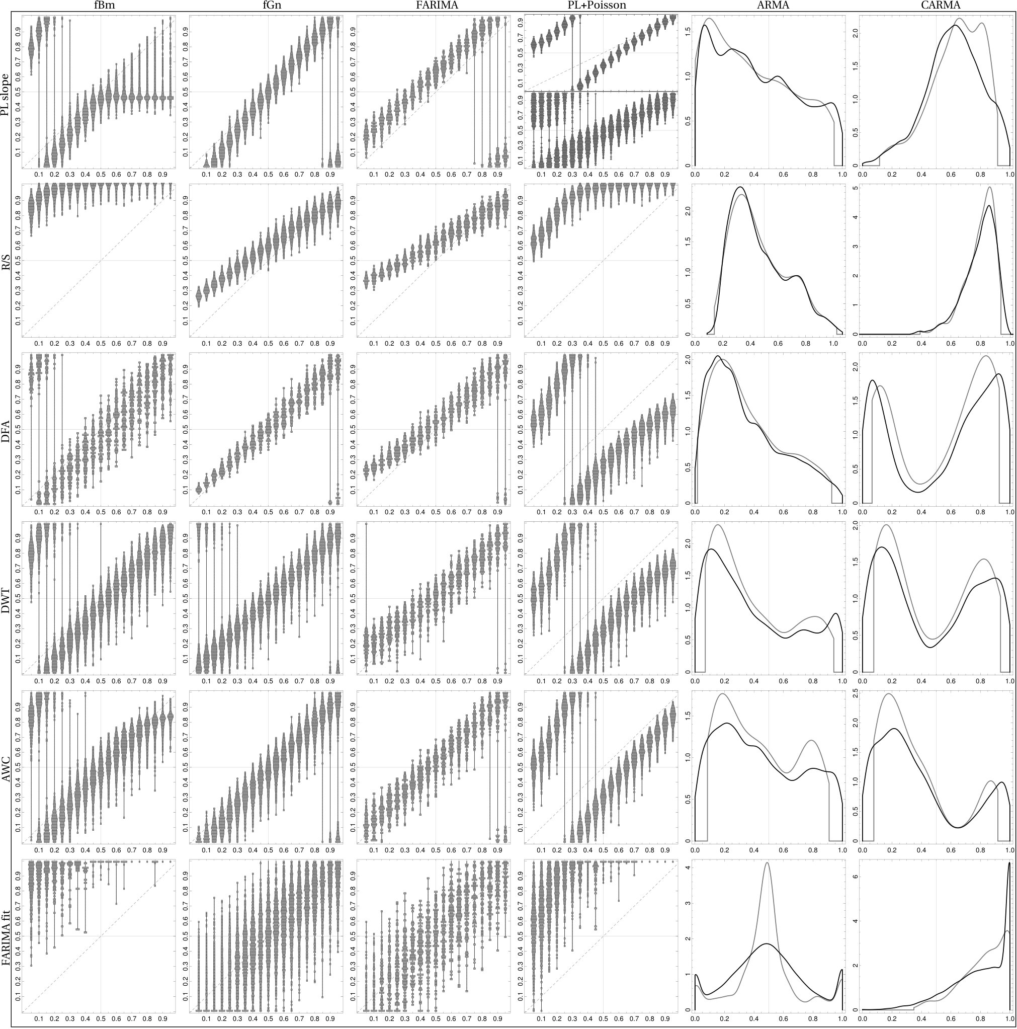
No single algorithm turns out to be best; some work well for a particular stochastic process, but fail miserably for others, e.g. fitting a PL rarely gives the correct estimate for fBm, but works quite well for fGn. The R/S method significantly overestimates for all examined processes except for ARMA ones, and fails completely for nonstationary fBm (North & Halliwell 1994; Gilmore et al. 2002). Likewise, it overestimates for CARMA processes. DFA, DWT and AWC give consistent and roughly correct results for processes with a nearly PL PSD (i.e. fBm, fGn, and FARIMA), but miss the correct in case of ARMA and CARMA. Fitting a FARIMA model and inferring the value of from the obtained works well for fGn, FARIMA and ARMA, although with a big dispersion around the correct value. However, for nonstationary processes it clusters at . This issue might be resolved by differencing, though, as discussed in Sect. IV.3. In many cases one can observe that very high and very low values lead to improper characterization of the time series, resulting in drastic misclassification, e.g. the DFA tends to return a very high for processes with very low input . Finally, the PSD of CARMA process [Eq. (39)] cannot be considered to be a PL even approximately (for the employed sets of parameters and frequency ranges of the PSDs), hence the long-term dependence is difficult to assess.
We therefore recommend to employ simultaneously a few algorithms when computing and examine the consistency of the obtained estimates. The shape of the investigated time series’ PSD should be also evaluated to justify the presence of long-term dependence before any attempts to extract are undertaken.
IV.6 plane
In Sect. III.7, the plane was described, and the locations of different processes with PSDs of PLC form were displayed in Fig. 7. Herein we investigate what regions of the plane is occupied by some other stochastic processes considered in this work.
We examine the family of ARMA processes, with . We generate sets of AR and MA coefficients, drawn uniformly from the regions of the parameter space of the AR coefficients that ensure stationarity, with MA coefficients drawn from and compute the locations . Results are displayed in Fig. 14. We also checked whether the regions occupied by each process change when the coefficients are drawn from a distribution, and find that the boundaries are the same.

The ARMA process is just white noise, so it clusters around . The PSD of ARMA is a close approximation to a PL, hence its values closely follow the true PL line depicted in the plots, deviating only for . We emphasize that the pure PL line follows the fBm line (Tarnopolski 2016; Zunino et al. 2017; Tarnopolski 2019a). Other ARMA models spread out into larger parts of the plane, with less internal structure for higher orders. See (Tarnopolski 2019a) for an analytic treatment of the regions of availability for ARMA processes, as well as fBm and fGn.
V Results
V.1 Fourier spectra
The Fourier spectra were generated and binned, as described in Sect. III.1, for each of the 7, 10, and 14 d binnings. Next, Eq. (12) and (13) were fitted in each case1616 16 We checked also the smoothly broken PL, where a transition between PLs with low- and high-frequency indices and occurs at a break frequency (see Żywucka et al. 2020), but it was not competing in any instance.. The better model was chosen based on the values; if they obeyed , we chose the pure PL model as the adequate one since it is simpler. The resulting indices and their standard errors are gathered in Table 2; plots of the best fits are displayed in Fig. 15. The PSDs of FSRQs are steeper than those of BL Lacs. Most of the objects gave consistent estimates among the three bins, except for Mrk 5011717 17 This source is dim, hence its variations are dominated by the observational (Poisson) noise., which yielded a wide range: 1.96, 2.53, and 1.73. Nevertheless, the PSDs are systematically flatter than in a red noise case, , with a mean of 1.19 and standard deviation of 0.43. One BL Lac, PKS 2155304, exhibits , i.e. is significantly flatter than pink noise, . On the other hand, two FSRQs, B2 1520+31 and B2 1633+38, are steeper than pink noise, yielding . The remaining objects, both BL Lacs and FSRQs, are very close to a pink noise description.
| Source | 7 d | 10 d | 14 d |
|---|---|---|---|
| (1) | (2) | (3) | (4) |
| BL Lacs | |||
| Mrk 501 | |||
| Mrk 421 | |||
| PKS 0716+714 | |||
| PKS 2155304 | |||
| TXS 0506+056 | |||
| FSRQs | |||
| PKS 1510089 | |||
| 3C 279 | |||
| B2 1520+31 | |||
| B2 1633+38 | |||
| 3C 454.3 | |||
| PKS 1830211 | |||
Note. — APure PL.
BPLC.
Columns: (1) source name; (2) for 7 d binning; (3) for 10 d binning; (4) for 14 d binning.
As demonstrated in Sect. IV.1, extracting the parameters of Eq. (13) from a number of realizations of the same process leads to a wide range of results, obscuring the true underlying process. Hence, the obtained values of are not entirely reliable. On the other hand, except for Mrk 501, employing different binnings gave highly consistent results, and in most cases it turned out that the Poisson noise did not influence the PSDs much, i.e. a pure PL was chosen as the better description. To test the robustness, from each LC we generated 1000 MC realizations by drawing the observations randomly from , where is the observed value, and is its standard error. That is, we produced 1000 stochastic realizations of the LCs allowed by the observable uncertainties. The results of such procedure are gathered in Table 3, where we display the mode and standard deviation of the resulting distributions of best-fit indices , and the mode of their standard errors , which we interpret as a typical error.
| Source | 7 d | 10 d | 14 d | ||||||
|---|---|---|---|---|---|---|---|---|---|
| mode | std | typ. err. | mode | std | typ. err. | mode | std | typ. err. | |
| (1) | (2) | (3) | (4) | (5) | (6) | (7) | (8) | (9) | (10) |
| BL Lacs | |||||||||
| Mrk 501 | 1.61 | 0.17 | 0.25 | 2.07 | 0.27 | 0.52 | 1.74 | 0.33 | 0.32 |
| Mrk 421 | 0.80 | 0.03 | 0.15 | 0.84 | 0.04 | 0.23 | 0.74 | 0.06 | 0.24 |
| PKS 0716+714 | 0.89 | 0.02 | 0.20 | 0.88 | 0.04 | 0.24 | 0.87 | 0.04 | 0.31 |
| PKS 2155304 | 0.57 | 0.07 | 0.11 | 0.52 | 0.11 | 0.09 | 0.64 | 0.08 | 0.11 |
| TXS 0506+056 | 1.94 | 0.42 | 0.20 | 0.75 | 0.67 | 0.18 | 0.82 | 0.39 | 0.21 |
| FSRQs | |||||||||
| PKS 1510089 | 0.97 | 0.06 | 0.08 | 1.03 | 0.02 | 0.08 | 1.02 | 0.02 | 0.11 |
| 3C 279 | 1.05 | 0.02 | 0.07 | 1.12 | 0.04 | 0.15 | 1.13 | 0.03 | 0.08 |
| B2 1520+31 | 1.72 | 0.13 | 0.11 | 1.26 | 0.19 | 0.11 | 1.28 | 0.15 | 0.11 |
| B2 1633+38 | 1.05 | 0.06 | 0.14 | 1.08 | 0.08 | 0.17 | 1.18 | 0.04 | 0.18 |
| 3C 454.3 | 1.50 | 0.04 | 0.15 | 1.54 | 0.08 | 0.16 | 1.59 | 0.06 | 0.16 |
| PKS 1830211 | 0.90 | 0.07 | 0.14 | 0.94 | 0.06 | 0.16 | 1.03 | 0.07 | 0.19 |
Note. — Columns: (1) source name; (2) mode of the distribution for 7 d binning; (3) standard deviation of the distribution for 7 d binning; (4) typical error, i.e. mode of the distribution for 7 d binning; (5) mode of the distribution for 10 d binning; (6) standard deviation of the distribution for 10 d binning; (7) typical error, i.e. mode of the distribution for 10 d binning; (8) mode of the distribution for 14 d binning; (9) standard deviation of the distribution for 14 d binning; (10) typical error, i.e. mode of the distribution for 14 d binning.
The values of from both Tables 2 and 3 are in agreement, hence the uncertainties of the flux do not play an important role in estimating . However, it is crucial to emphasize that this only means that the estimates of the PL parameters for a given LC can be trustworthy when it comes to impact of the errors on the outcome. Still, this particular time series might be a peculiar realization of the process governing the observed variability, and need not represent the true parameters ultimately. In fact, as implied by the benchmark testing from Sect. IV.1, the mismatch between the (unknown) true value and the extracted one can be severe, especially when Poisson noise constitutes a significant component in the PSD.
V.2 Lomb-Scargle periodograms
The same analysis as in Sect. V.1 was performed with the LSP (see Sect. III.2). The fitted indices are gathered in Table 4; plots of the best fits are displayed in Fig. 15. The values of are slightly lower, and their errors are smaller than obtained by fitting Fourier spectra. The latter is caused by the ability of the LSP to generate PSDs with larger number of points, hence constraining the fits better. In Table 5 the results of MC realizations drawn by varying the LC values within the error bars are displayed. We arrive at a similar conclusion as in Sect. V.1, i.e. the uncertainties of the flux do not affect the estimated PSD shape significantly. We repeat, though, that the PL parameters depend strongly on the particular realization of a time series, as was demonstrated in Sect. IV.1.
| Source | 7 d | 10 d | 14 d |
|---|---|---|---|
| (1) | (2) | (3) | (4) |
| BL Lacs | |||
| Mrk 501 | |||
| Mrk 421 | |||
| PKS 0716+714 | |||
| PKS 2155304 | |||
| TXS 0506+056 | |||
| FSRQs | |||
| PKS 1510089 | |||
| 3C 279 | |||
| B2 1520+31 | |||
| B2 1633+38 | |||
| 3C 454.4 | |||
| PKS 1830211 | |||
Note. — APure PL.
BPLC.
Columns: (1) source name; (2) for 7 d binning; (3) for 10 d binning; (4) for 14 d binning.
| Source | 7 d | 10 d | 14 d | ||||||
|---|---|---|---|---|---|---|---|---|---|
| mode | std | typ. err. | mode | std | typ. err. | mode | std | typ. err. | |
| (1) | (2) | (3) | (4) | (5) | (6) | (7) | (8) | (9) | (10) |
| BL Lacs | |||||||||
| Mrk 501 | 1.86 | 0.27 | 0.23 | 2.42 | 0.33 | 0.26 | 2.12 | 0.37 | 0.30 |
| Mrk 421 | 0.85 | 0.08 | 0.07 | 0.83 | 0.11 | 0.09 | 0.77 | 0.30 | 0.09 |
| PKS 0716+714 | 0.90 | 0.02 | 0.09 | 0.91 | 0.04 | 0.11 | 0.97 | 0.03 | 0.12 |
| PKS 2155304 | 0.56 | 0.05 | 0.09 | 0.56 | 0.26 | 0.10 | 0.62 | 0.08 | 0.12 |
| TXS 0506+056 | 2.09 | 0.20 | 0.32 | 2.12 | 0.30 | 0.34 | 1.96 | 0.24 | 0.29 |
| FSRQs | |||||||||
| PKS 1510089 | 0.91 | 0.06 | 0.07 | 0.95 | 0.03 | 0.08 | 0.94 | 0.03 | 0.10 |
| 3C 279 | 1.05 | 0.02 | 0.09 | 1.12 | 0.04 | 0.11 | 1.13 | 0.03 | 0.12 |
| B2 1520+31 | 1.36 | 0.16 | 0.19 | 1.07 | 0.12 | 0.08 | 1.09 | 0.12 | 0.09 |
| B2 1633+38 | 1.49 | 0.15 | 0.16 | 1.58 | 0.12 | 0.18 | 1.61 | 0.21 | 0.19 |
| 3C 454.3 | 1.94 | 0.09 | 0.25 | 2.08 | 0.10 | 0.24 | 2.08 | 0.13 | 0.24 |
| PKS 1830211 | 1.03 | 0.05 | 0.10 | 1.09 | 0.04 | 0.11 | 1.13 | 0.04 | 0.12 |
Note. — Columns: (1) source name; (2) mode of the distribution for 7 d binning; (3) standard deviation of the distribution for 7 d binning; (4) typical error, i.e. mode of the distribution for 7 d binning; (5) mode of the distribution for 10 d binning; (6) standard deviation of the distribution for 10 d binning; (7) typical error, i.e. mode of the distribution for 10 d binning; (8) mode of the distribution for 14 d binning; (9) standard deviation of the distribution for 14 d binning; (10) typical error, i.e. mode of the distribution for 14 d binning.
We also note that the PSDs of Mrk 501 behave in an unorganized manner—i.e., the spread of their is wide, and the values do not overlap within errors. In particular, for the 10 d binning the PSD is steepest. This is most likely due to it being a dim object, where the variability is obscured by observational fluctuations and statistical noise. Despite visually similar LCs among the three binnings, we clearly observe that the fitted form of the PSD is strongly dependent on the particular stochastic realization, in agreement with our findings from Sect. IV.1.
V.3 Wavelet scalograms
We detect a well-known QPO in PKS 2155304, at a period of days1818 18 For comparison with previous works (Sandrinelli et al. 2014; Sandrinelli et al. 2016; Zhang et al. 2017a) a Gaussian form was fitted to the corresponding peak in the LSP of the 7 d binned LC, and the error is the half width at half maximum. Applying the same procedure to the peak in the global wavelet periodogram yielded days. (Fig. 16). This period is smaller than reported by previous works (650–660 days by Sandrinelli et al. 2014; 642 days by Sandrinelli et al. 2016; 635 days by Zhang et al. 2017a), but consistent with more recent ones (610 days by Bhatta & Dhital 2020). Peñil et al. 2020 reported 620 days in a 28-day binned LC. Overall, a linear decrease over the years can be observed. The QPO is unambiguous in the 7 d binned LC examined herein, partially disappears in the 10 d binned LC, but is not present at all in the 14 d binned LC. Additionally, when considering the global wavelet periodograms alone, PKS 1830211 in the 7 d binning shows a marginal peak just above the confidence level. This peak, however, can be attributed to two short-lasting contours of significance in the scalogram, at the borders of the COI. These contours correspond to apparently different periods. One can associate these contours with short, two-peak flux variations in the LC. They are however so short-lasting that cannot be called QPOs—if so, they would consist of only two cycles each, which is likely just a chance occurence owing to stochastic fluctuations, and definitely does not constitute a significant QPO detection. There is also a contour at an even higher period, days, but its duration is comparable to its period. Overall, there is no convincing evidence to claim a QPO in PKS 1830211, especially when compared to the picture painted by PKS 2155304.
There is a peculiar feature in B2 1633+38, with a contour starting at days, and increasing over the course of the LC to days. The two peaks in the global periodograms, at 634 and 1066 days, are spurious in the sense that they arise due to this one structure that evolves strongly in time. This might be called a QPO, with an emphasis of the quasi term, as no single leading period can be associated with it.


V.4 ARMA and FARIMA modeling
To estimate the long time scales breaks of the ARMA fits, we first observe that the obtained PSDs’ shapes resemble the Lorentzian from Eq. (40), i.e. they are flat at low frequencies, and then transition to an approximately PL decay (see the middle panels in Fig. 17). The general PSD of an ARMA process, Eq. (37), is not given by a combination of Lorentzian peaks1919 19 For some values of the parameters the PSD can be completely non-Lorentzian, e.g. monotonically increasing., though, so we proceed numerically in a way driven by an analogy with the simple Lorentzian shape. It is straightforward to check that has its break at the same frequency as has its local maximum. We therefore locate the first local maximum of and identify it with the break frequency. To compute the uncertainties, the parametric bootstrap is employed (Tarnopolski 2015b, and references therein): we generate 500 PSDs by varying randomly the coefficients of the best-fit ARMA model within their errors, and take the standard deviation of the distribution of breaks as the standard error.
The ARMA models were fitted using the method of moments first. For choosing the best fit, we employed , because, as implied by the benchmark testing from Sect. IV.3, it is more likely to return if not , then at least close to the real value when noise is present in the observations. In particular, the best model is chosen to be the one with smallest within the band . The outcomes of this method are gathered in Table 6. However, as demonstrated in Appendix A, the maximum likelihood estimation is prone to underestimate the order. In most instances the results do not match: was the most commonly returned order, with occasional , , (, or . On one hand, the method of moments is more likely to point at a plausible model as indicated by the testing from Sect. IV.3; on the other, the higher-order models, e.g. ARMA in case of Mrk 501 or TXS 0505+056 (Fig. 17), but also B2 1510+31, B2 1633+38, PKS 2155304, are modeling the variations at the Poisson noise level, hence are likely overfitting, i.e. are modeling the fluctuations related to uncertainties in the data, and hence their order is superficially elevated to take this into account, and does not entirely reflect the features of the underlying process that governs the variability.
Note that , as noted in Sect. II.4, is more liberal than , hence points at unnecessarily complex models. In case of the examined blazars, it returned as high as or . All in all, the combination of method of moments and gives the most reliable description of the LCs at hand, and hence we proceed to discuss them.
| 7 d | 10 d | 14 d | ||||
|---|---|---|---|---|---|---|
| Source | ||||||
| [day] | [day] | [day] | ||||
| (1) | (2) | (3) | (4) | (5) | (6) | (7) |
| BL Lacs | ||||||
| Mrk 501 | ||||||
| Mrk 421 | ||||||
| PKS 0716+714 | ||||||
| PKS 2155304 | ||||||
| TXS 0506+056 | ||||||
| FSRQs | ||||||
| PKS 1510089 | ||||||
| 3C 279 | ||||||
| B2 1520+31 | ||||||
| B2 1633+38 | ||||||
| 3C 454.3 | ||||||
| PKS 1830211 | ||||||
Note. — Columns: (1) source name; (2,4,6) orders for 7, 10 and 14 d binnings; (3,5,7) corresponding long break time scales.
In the defining Eq. (29) of the ARMA process, the observation is directly influenced by preceding ones. For example, let in an LC with a 7 d binning. This means that the observations from the previous 28 days (in the observer frame) affect the current value. For an LC with a 14 d binning one can then expect in order to maintain the same time scale . We see exactly this pattern in case of B2 1633+38 (Table 6).
The PSDs are presented in Fig. 17. Mrk 501 (in the 10 d binning) yields ARMA. At higher frequencies (corresponding to timescales ) we observe local maxima above the Poisson noise level—these might be either QPOs, or just fluctuations—especially that wavelet scalograms show no signs of QPOs at all (Sect. V.3). In case of TXS 0506+056 (for all binnings) the high-frequency variations are exactly at the Poisson noise level. PKS 1830211 consistently exhibits a prominent break in its PSD at a time scale of several hundred days (see Table 6). On the other hand, Fourier spectra and LSPs do not hint at any break (compare with Sect. V.1 and V.2).
Overall, we observed breaks at time scales of a few hundred days in all but the following objects: B2 1520+31 (for which we obtain very big uncertainties), and 3C 454.3 (for which the breaks correspond to very long time scales, as the PSD of this source is highly consistent with a pure PL). The most pronounced and well-constrained breaks occur in Mrk 421, PKS 2155304, PKS 1510, and 3C 279. The break time scales are generally consistent with break timescales obtained by CARMA modeling (see Sect. V.5). This equivalence is to be expected, as CARMA is just a continuous-time version of ARMA, and the data herein are nearly uniformly sampled, with not many missing points, hence the two models ought to give similar results.
V.5 CARMA modeling
Ryan et al. 2019 recently investigated daily and weekly LCs of eight blazars examined herein as well, except for Mrk 501, TXS 0506+056, and PKS 1830211, by fitting CARMA models, , and found that in all cases or give the best fits. We performed a broader search for and . We employ , and choose the simplest model (i.e., with lowest ) within the band as the best fit. Our results, summarized in Table 7, are generally in agreement with Ryan et al. 2019. In the case of 7 d binning of PKS 2155304, when restricted only to CARMA, we also obtain as the best, and as the simplest model within . Likewise for PKS 1830211 in a 7 d binning. In these two fittings, however, the orders exceeding appear to be spuriously elevated to take into account subtle variations below the Poisson noise level, hence imply overfitting. Indeed, when the higher-order and simple models are compared (Fig. 18), they all exhibit PSDs broadly consistent with each other within the confidence intervals.
In particular, almost all fits are in fact consistent with the simplest, CARMA model, as in the case of CARMA fits the second break in the PSD is mostly located below the Poisson noise level. The only exception is 3C 279, with breaks at and days (see Fig. 19). Curiously, the 8.5-years-long Fermi-LAT LC of the famous source OJ 287 exhibits a break at 150 days in a CARMA best fit (Goyal et al. 2018).
| 7 d | 10 d | 14 d | |||||||
|---|---|---|---|---|---|---|---|---|---|
| Source | |||||||||
| [day] | [day] | [day] | [day] | [day] | [day] | ||||
| (1) | (2) | (3) | (4) | (5) | (6) | (7) | (8) | (9) | (10) |
| BL Lacs | |||||||||
| Mrk 501 | |||||||||
| Mrk 421 | — | — | — | ||||||
| PKS 0716+714 | — | — | — | ||||||
| PKS 2155304 | — | — | |||||||
| TXS 0506+056 | |||||||||
| FSRQs | |||||||||
| PKS 1510089 | — | — | — | ||||||
| 3C 279 | — | — | |||||||
| B2 1520+31 | — | — | |||||||
| B2 1633+38 | — | — | — | ||||||
| 3C 454.3 | — | — | — | ||||||
| PKS 1830211 | — | — | |||||||
Note. — Columns: (1) source name; (2,5,8) orders for 7, 10 and 14 d binnings; (3,6,9) long time scale breaks; (4,7,10) short time scale breaks.
aThis was returned as the best order, but the given and refer to a CARMA fit.
bBelow the Poisson noise level.
cFor CARMA, , effectively implying no break.
The fits to Mrk 501, TXS 0506+056, PKS 1830211 are featureless, with at very long time scales, making the PSDs consistent with a PL description. In particular, there are no signs of a QPO in case of PKS 1830211, contrary to what the global wavelet periodogram (7 d binning, Sect. V.3) might suggest. In conclusion, we did not detect any peculiar features in the PSDs obtained with fitting CARMA models to our data. The break time scales that are above the Poisson noise level are either at a few hundred, or several thousands of days.
V.6 Hurst exponents
We used all methods from Sect. III.6 to estimate the Hurst exponents. The results are summarized graphically in Fig. 20. In some instances, fitting a FARIMA model returned (leading to ), which implies nonstationarities present in the respective LCs. As illustrated in Fig. 13, FARIMA fitting is biased towards higher when applied to PLC (and even more biased in case of fBm); it has a great dispersion when used at fGn and FARIMA models; and while usually recovers correctly for ARMA, it can drift towards or ; finally, for CARMA models it consistently returns close to . Therefore, not much meaning can be given to the estimates from FARIMA fitting (Torre et al. 2007).
On the other hand, the Fourier spectra and LSPs yielded for many objects , which due to the discoutinuity of at the border between stationary and nonstationary processes (see Fig. 6) makes it uncertain whether or . Only Mrk 501, PKS 2155304, B2 1520+31, and B2 1633+38 are far enough from the border to allow to confidently infer from (Tables 2 and 4). However, as Mrk 501 gives inconsistent for different binnings, the corresponding span the range . For PKS 1510089, Fourier spectra lead to , while LSPs yield .
The AWC often drifts to , which is a nonsensical value. Overall, it systematically returns . Its performence for PLC (see Fig. 13) is poor, and it greatly misidentifies as when nonstationarities are present, e.g. in the fBm case, so technically also for . The performance of the R/S algorithm is also poor and hence unreliable. What is left is only DFA and DWT.
We undertook the following approach in order to try to differentiate between and . Given a time series of length , it was divided into windows of size . The first window starts at , the second advances one points and starts at , etc. We end with such chunks, to each we apply the DFA algorithm, and eventually obtain the time evolution of . The values for each LC and binning will vary over time, but we aim at seeking a general answer whether or , or it oscillates discontinuously between and . The results are gatherdd in Fig. 21, where also the time evolution of and is displayed (see Sect. V.7).
We indeed confirm that for blazars characterized by , the values behave incoherently in time. For the most part, Mrk 501 and TXS 0506+056 actually exhibit , implying long term memory. PKS 2155304 is the best behaving object, with the time evolution of consistent in all three binnings. We observe jumps between and for B2 1520+31 and B2 1633+38, suggesting that the estimates obtained in Sect. V.1 and V.2 do not capture the true stochastic dynamics of the system. We can safely conclude that long range dependence is rather confidently detected in the LC of PKS 2155304, and likely also for Mrk 501 and TXS 0506+056. On the other hand, 3C 454.3 is the only object for which is consistently returned, in agreement with , suggesting its variability is fBm-like with short-term memory.
V.7 The plane
The locations in the plane were calculated according to Sect. III.7. To constrain the errors, from each LC we generated 1000 MC realizations by drawing the observations randomly from , where is the observed value, and is its standard error, and for each realization the location was computed. The dispersion is assessed by the standard deviation of the 1000 MC samples. The results are displayed in Fig. 22, where the region available to generic PLC models is highlighted. As per Sect. V.1 and V.2, the majority of the examined blazars are well described by a pure PL: Mrk 421, PKS 0716+714, PKS 2155304, PKS 1510089, and 3C 279, using both Fourier spectra and LSPs. Four of them are close to a pink noise PL with , except for PKS 2155304, which yields . The locations are roughly consistent with , but generally shifted towards slightly steeper PL PSDs. This is in agreement with the underestimation of the indices observed in the benchmark tests in Sect. IV.1. Note however that in case of Mrk 421 we observed a slight, and in case of PKS 2155304 a strong shift upwards the plane.
Mrk 501 is a source that is most shifted to the right and upwards, which is due to a high level of Poisson noise dominating the PL component in a substantial part of its PSD. The result of increasing the Poisson noise (Fig. 7) is that the path for different is raised and shortened. Hence the locations are shifted closer to the point corresponding to white noise. Therefore, overall the description of Mrk 501 in the plane is reasonable.
Finally, B2 1520+31 and B2 1633+38 yield , but for some binnings the PSDs were better described by a PLC rather than a pure PL. They behave differently in the plane: for higher binnings, B2 1520+31 moves vertically upwards, while 1633+38 moves diagonally to the right and downwards. The latter appears to be more consistent with a pure PL location; for the 10 binning there is strong support for the pure PL model in the LSP approach (). For the 7 d binning of B2 1520+31, though, the pure PL is out of question, with in the Fourier approach, and in case of LSP, what means inconsiderable support for the pure PL model.
Recall that the LCs, despite spanning a long period in time, contain a moderate number of points, especially for the 10 d and 14 d binnings. On the other hand, the 7 d binning allows for a denser sampling, but increases the uncertainty of the measurements.
VI Discussion
VI.1 Summary of results
We analyzed with a number of techniques the Fermi-LAT -ray LCs of 11 blazars. The global PSDs were obtained via Fourier spectrum and the LSP, and subsequently used to compute the PL indices . The values resulting from these methods are consistent with each other (see Tables 2 and 4). There is a small discrepancy only in case of 3C 454.3, for which the Fourier PSD is described by a pure PL, and the LSP by PLC—the latter being slightly steeper than the former. Overall, the resultant shapes indicate a colored noise with .
We employed wavelet scalograms to detect transient phenomena. We confirmed the well-known QPO in PKS 2155304, with a period of days. We did not find any other similarly unambiguous QPOs at the confidence level. B2 1633+38 exhibits a peculiar, significant feature that evolves from days to days over the span of the LC, that might be associated with the previously reported presumed QPOs with days (Otero-Santos et al. 2020). Additionally, there is a peak in the global wavelet PSD in the 7 d binned LC of PKS 1830211. This, however, appears to be a dubious detection, as the statistically significant features in the scalogram are located exactly at the border of the COI, at two different frequencies, and can be identified with at most two cycles in the LC. Moreover, there is no significant detection in 10 and 14 d binned LCs of this source. We therefore conclude a lack of significant QPOs in the remaining sample of blazars. In particular, we cannot confirm the presence of QPOs in Mrk 501 (Bhatta 2019), Mrk 421 and PKS 0716+714 (Bhatta & Dhital 2020), PKS 1510089 and 3C 279 (Sandrinelli et al. 2016), and B2 1520+31 (Gupta et al. 2019) (compare with Table 1). Finally, we observe hints of a significant, persistent structure in the scalograms of PKS 0716+714 at days. This might be a candidate QPO, but since the ratio of the period to the length of the LCs allows for 2–3 cycles only, it does not constitute a detection yet. Similar conclusions were drawn by Bhatta & Dhital 2020, while Peñil et al. 2020 reported a low-significance QPO detection at a period of 1000 days. Further monitoring of this source is therefore required.
We modeled the LCs as discrete stochastic processes, ARMA and FARIMA, fitting them with the method of moments and by maximum likelihood estimation. The latter yielded simple, low order models. The method of moments, however, in some instances (Mrk 501, PKS 0716+714, PKS 2155304, B2 1520+31, B2 1633+38) returns higher orders. For most of them (Mrk 501, PKS 2155304, B2 1520+31, B2 1633+38) the increased model complexity is caused by overfitting at the Poisson noise level. On the other hand, PKS 0716+714 shows nontrivial features significantly above the Poisson noise level, and hence hints at a more complicated process underlying the observed variability.
The LCs were modeled as CARMA processes as well (Table 7). We searched for the best CARMA model with and . In almost every instance we obtained the orders or . In only a few cases the pointed at more complex models, but their PSDs are consistent with these simple instances (see Fig. 18 and 19), as the additional parameters introduced by higher orders were utilized for overfitting below the Poisson noise level. We are therefore in agreement with the results of Ryan et al. 2019 when it comes to the eight blazars common to both works. Additionally, the CARMA fits to Mrk 501, TXS 0506+056, and PKS 1830211 are consistent with a PL description, i.e. CARMA with a high .
Nevertheless, motivated by the fact that the proper model to describe the data may not necessarily be a simple PL, we estimated the Hurst exponents with several of the most popular and established methods. For most BL Lacs we obtain significantly, signifying long-term memory. The FSRQs, however, kept oscillating between and , except 3C 454.3 for which convincingly. We emphasize, though, that some of the objects (Mrk 421, PKS 0716+714, and most FSRQs) do not allow to formulate an unambiguous claim about their persistence: there is no convincing majority of consistent estimates to infer whether . This is in accordance with the fact that their PSDs are highly consistent with a PL description with : due to the discontinuity of (see Fig. 6) it is difficult to distinguish between stationary cases with and nonstationary with . We note that it might be proper to model the LCs as a CARFIMA process (Tsai & Chan 2005; Tsai 2009; Feigelson et al. 2018), i.e. a fractionally integrated CARMA process (or, in other words, a continuous-time FARIMA) that allows for long-term memory, as well as CARMA driven by a Lévy process (Brockwell 2004; Brockwell & Marquardt 2005). Likewise, the fractional Fokker-Planck equation admits long-term memory solutions (Weron et al. 2008; Deng & Barkai 2009), and might be used to model the electron distribution (Stawarz & Petrosian 2008; Chen et al. 2011), thus constitutes a generalization of the kinetic continuity equation (Finke & Becker 2014; Finke & Becker 2015).
In regards to the memory of the process, consider again the orders of the ARMA models. If the observed variability is caused by some (possibly recurring) disturbance in the jet or disk, it will need some time to dissolve. One can then expect that increasing the binning of an LC twice will reduce the ARMA order twice as well, which is indeed the case for some blazars (Sect. V.4). The relation between the rest and observer frames is . In particular, for B2 1633+38 (7 d binning; as per Table 6), transforms to 10 days in the rest frame. A decrease of the order with the increase of the bin size is also evident, although less clear, for PKS 0716+714, PKS 2155304, B2 1520+31, to which we relate , 19, and 14 days, assuming , according to the orders for a 7 d binning. Such a relation suggests there might exists a characteristic time scale for the perturbations to die out, i.e. any fluctuation in the jet affects the emission for time . Physical differences in the blazars, e.g. BH mass, accretion rate etc. could lead to different .
Finally, we highlight a novel finding made with the recently introduced plane: the FSRQs and BL Lacs are clearly separated, as shown in Fig. 22. The FSRQs are characterized by lower values of than BL Lacs. The same phenomenon was also discovered by Żywucka et al. 2020 in the optical (I band) light curves of blazar candidates behind the Magellanic Clouds (Żywucka et al. 2018), observed by the Optical Gravitational Lensing Experiment (OGLE). This demonstrates that the interrelations between flux values are different for the two blazar populations, and allows to distinguish them based solely on data in the time domain, without referring to PSDs or spectroscopic properties. Moreover, the separation is insensitive to sampling: the blazar candidates from Żywucka et al. 2020 were observed irregularly, with a time step approximately a multiple of 1 d, while the -ray LCs examined herein were binned into 7 d, 10 d, and 14 d intervals.
The separation, at first glance, might appear to be a result of FSRQs having on average steeper PSDs than BL Lacs. This is not the case: this would be true if all objects were located at the pure PL line in the plane, and their locations would be consistent with the estimates. However, the examined sources attain various values of , too, sometimes placing them far from the PL line. In effect of adding Poisson noise, the PL line is elevated and shortened, i.e. pulled closer to the point corresponding to white noise. Such a path is depicted in magenta in Fig. 22, and it does not separate the two classes at all. Most of the blazars’ PSDs herein are consistent with a pure PL, though, hence the location in the plane highlights some hidden properties in the time series’ temporal structure, not revealed by Fourier spectra or LSPs. Moreover, the region of availability for PSDs of PLC is also available to ARMA processes (see Fig. 14, and Tarnopolski 2019a for an analytic treatment).
VI.2 Comparison with previous studies
PL indices
Nakagawa & Mori 2013 analyzed almost 4-years-long LCs of 15 blazars from the Monitored Source List (MSL), provided by the Fermi-LAT team, using the Fourier transform. Their sample contains five blazars the same as in our work, i.e. Mrk 421, 3C 279, PKS 1510089, PKS 2155304, and 3C 454.3. The PL indices of the considered blazars are compatible with our results within errors, except for Mrk 421, for which we obtained a steeper PSD ( vs. ). 13 blazars, with particular emphasis on blazar types, i.e. eight FSRQs and five BL Lacs, were analyzed by Sobolewska et al. 2014 with a superposition of OU processes. Their sample also includes a bunch of blazars studied in this work: B2 1633+38, B2 1520+31, 3C 454.3, 3C 279, PKS 1510089, PKS 0716+714, PKS 2155304, and Mrk 421, for which they find PL indices mostly to be . There is also no difference in values among the two blazar types. Abdo et al. 2015 studied a 3-years-long LC of PKS 1830211, generated with the unbinned maximum likelihood technique. Our Fourier PSD is slightly flatter than theirs ( vs. ). The 7-years-long LCs (calculated with unbinned maximum likelihood method) of three blazars were analyzed by Kushwaha et al. 2017. Common objects in this case are Mrk 421, B2 1520+31, and PKS 1510089. The PL index of Fourier PSDs is in an agreement only for PKS 1510089, while for Mrk 421 and B2 1520+31 we obtained flatter and steeper PSDs, respectively. Prokhorov & Moraghan 2017 for PKS 0716+714 obtained , and for PKS 2155304, while we obtain and . They get within , though, for all their sources. Algaba et al. 2018 analyzed a 3-years-long LC of B2 1633+382, generated with the adaptive binning method, to study its variability in radio, optical, and HE -rays. Here again the fitted PL is flatter in our case ( vs. ). Bhatta 2019 investigated a 10-years-long LC of Mrk 501, generated with unbinned maximum likelihood method, finding a PL index of , which is much flatter than the value found in this work (). Covino et al. 2019 examined long-term (decade), 30 day-binned aperture photometry LCs generated by the Fermi team of 10 blazars, including PKS 0716+714 and PKS 2155304. Our PL index is comparable in case of the former blazar, but gives a flatter PSD for the latter one. Subsequently, Meyer et al. 2019 investigated 9.5-years-long, weekly-binned LCs of six FSRQs, including PKS 1510089, 3C 279, and 3C 454.3. Except for PKS 1510089, they obtained clearly flatter PL fits than we do, i.e. vs. our (Fourier PSDs) or (LSPs), respectively. Our results are consistent with Bhatta & Dhital 2020, except for 3C 454.3, for which the authors reported , while we obtained . Finally, regarding Mrk 421 and PKS 2155304, we obtained values broadly consistent with those of Goyal 2020.
All discrepancies highlighted here are most likely caused by different methods of data analysis, e.g. the methods of generating and fitting the PSDs, as well as differences in data itself, i.e. lengths of the analyzed LCs or method of their generation.
QPOs
Several authors reported QPOs in different blazars in recent years. Sandrinelli et al. 2014 analyzed long-term IR, optical, and HE -ray (MSL Fermi-LAT) LCs of PKS 2155304, with LSP and the Date Compensated Discrete Fourier Transform methods, finding a QPO with a period of 650 days in the GeV energy range. Afterwards, Sandrinelli et al. 2016 investigated similar data of six blazars, including 3C 279, PKS 1510089, and PKS 2155304, using LSPs. All objects showed QPOs in HE -ray LCs, at periods of 24 and 39 days with 3 significance in case of 3C 279, 115 days with 2.58 for PKS 1510089, as well as 642 days (3), 52 and 61 days (2.58) for PKS 2155304. Sandrinelli et al. 2017 studied optical and MSL Fermi-LAT data of three blazars, i.e. BL Lac, Mrk 421, and PKS 0716+714, using LSP and claiming no QPOs with significance 3. Zhang et al. 2017a generated 8-years-long Fermi-LAT LCs of PKS 2155304, using two methods: the maximum likelihood optimization and the exposure-weighted aperture photometry. The authors searched for QPOs with LSP and WWZ methods, finding a QPO with the period of 635 days at 4.9 significance level, thus confirming the QPO period found by Sandrinelli et al. 2014; Sandrinelli et al. 2016. We also confirm this QPO at 3 significance level, finding a period of days, consistent with a linear decrease of its value over the years.
The 7-years-long LCs of Mrk 421, PKS 1510-089, and B2 1520+31 were generated with unbinned likelihood analysis method by Gupta et al. 2019, and then QPOs were searched for applying LSP and WWZ techniques. A quasi-periodic signal was found only for B2 1520+31, with a period of 71 days with significance. We did not obtain any peculiar structures in the scalograms for this source. Covino et al. 2019 studied long-term (decade) MSL Fermi-LAT LCs, including PKS 0716+714 and PKS 2155304, finding no QPOs at a 3 significance level as well.
Bhatta 2019 generated a 10-years-long Fermi-LAT LC, using unbinned likelihood analysis. The LC was analyzed with the LSP and WWZ, showing a QPO with a period of 330 days, reaching a significance of 2.58. We did not observe any signs of this QPO at a 3 level in the scalograms, though. Likewise, we did not confirm the QPOs in Mrk 421 and PKS 0716+714, reported by Bhatta & Dhital 2020 on a <4 level.
Otero-Santos et al. 2020 analyzed the 11-years-long Fermi-LAT LC of B2 1633+38, generated with unbinned likelihood analysis, using three different techniques: the Discrete Correlation Function (DCF), LSP, and WWZ. They found a hint of QPOs with periods of 639 and 646 days at 2 level, with WWZ and LSP methods, respectively, as well as a more significant QPO at 3–4 having a period of 581 days with DCF. We obtained a peculiar structure in the scalograms of this blazar, evolving from days to days over the course of the LC, with 3 significance.
Discrepancies with previous analyses
Covino et al. 2019 analyzed blazars’ LCs generated by the Fermi-LAT team with the aperture photometry method, available on the LAT 3FGL Catalog Aperture Photometry Lightcurves webpage2020 20 https://fermi.gsfc.nasa.gov/ssc/data/access/lat/4yr_catalog/ap_lcs.php. These LCs constitute a quick-look facility to easily scan for interesting features in the data. At the same time it is strongly discouraged to use this data directly for the detailed scientific analysis, since the LCs can contain the emission from nearby sources. Also the fluxes may be affected by the background emission (point-like and/or diffuse). Similarly, Nakagawa & Mori 2013; Sandrinelli et al. 2014; Sandrinelli et al. 2016; Sandrinelli et al. 2017; Castignani et al. 2017; Ryan et al. 2019 studied the LCs accessible on the Monitored Source List Light Curves webpage2121 21 https://fermi.gsfc.nasa.gov/ssc/data/access/lat/msl_lc/ provided by the Fermi Science Support Center. Here again, the LCs are generated in an automatic way, using preliminary calibration and instrument response functions, to help searching for flares in the data and plan the follow-up analysis in other bands. It is not recommended to use this data in a scientific analysis as well.
Various authors adopted different significance levels for asserting the significance of QPO detections, ranging from , through arbitrary values like 95% or 99%, rarely exceeding (99.73%). E.g., Bhatta 2019 was the first to try to look for possible QPOs in the Fermi-LAT data of Mrk 501, finding a QPO with a period of 330 days. This is a very interesting result which, however, needs to be further verified, since this possible QPO was reported only on a significance level. Moreover, Gupta et al. 2019 claimed a QPO detection in B2 1520+31 merely on a level. The correct methodology is to set a goal, e.g. for finding a signal on a given significance level (though one that warrants a detection, i.e. at least ), and not report just any detected feature (especially with low significance). Moreover, sometimes a false alarm probability is reported (Sandrinelli et al. 2014) or used to set the significance (Gupta et al. 2019). This, however, tests a peak in the periodogram against a white noise model (VanderPlas 2018), while blazars exhibit PL-like PSDs, hence peaks exceeding the level against white noise will usually not be significant when tested against colored noise. Another issue is an abuse of the wavelet scalogram: while this is a powerful tool sensitive to transient phenomena in a time series, and therefore ideal to search for QPOs in blazar LCs, it is often used—with asserting the significance—as a global periodogram, like an LSP with which it is often highly consistent (Zhang et al. 2017a; Zhang et al. 2017b). A global periodogram is an average of the power at a given frequency among the whole LC. As was demonstrated in Sect. V.3, a scalogram can reveal that an apparently statistically significant peak in a global periodogram can signal a spurious quasiperiodicity, which is not supported when looking how the power among different frequencies is distributed in time. Unfortunately, in many works the scalogram is merely displayed, without performing any significance estimation (Zhang et al. 2017a; Zhang et al. 2017b; Bhatta 2019; Gupta et al. 2019; Otero-Santos et al. 2020) or even displaying the COI. We performed here such an estimation that allowed to conclude that any qusiperiodicity in our sample that might be claimed based on the global periodogram is spurious. While in some instances the scalogram is very convincing, e.g. in case of PG 1553+113 (Ackermann et al. 2015), still a significance analysis of its local features, not only global, is required. Finally, we stress again that a QPO, when present in the data, is not necessarily a signature of any periodic phenomena occuring in the system. Hence attributing a significant, constant period obtained from a global periodogram, with a true periodicity, is in our opinion unjustified. Indeed, the peaks observed in an LC can be spaced very nonuniformly, therefore a visual inspection of the LC for the presence of equidistant peaks can be misleading.
ARMA
The only attempt, to the best of our knowledge, to analyze -ray Fermi-LAT data with an ARMA model is the case of a BL Lac type object PKS 0301243, located at , using a 30 d binned LC (Zhang et al. 2017b). Fitting returned as the order, meaning that three previous observations affect any given flux value in the LC. This implies a characteristic time scale of days, which is substantially greater compared to our results. This is intriguing, since it suggests that such a time scale might differ among different blazars. Adding this source to B2 1633+38, PKS 0716+714, PKS 2155304, and B2 1520+31, produces a lack of correlation between and ( of PKS 0301243 taken from Ghisellini et al. 2010). When is calculated for all 11 of our blazars, with the best-fit orders for the 7 d binning, no correlation with can be inferred either. It appears that the BH mass is not a crucial parameter in influencing the values of . Further research on a bigger sample is therefore necessary for assessing the meaningfulness of such time scale regarding its physical origin.
It is worth to mention that the 22 and 37 GHz LCs of 3C 279 and 3C 454.3 were fitted with ARIMA models (Bewketu Belete et al. 2019), resulting in (i.e., once differenced to ensure stationarity), with for 3C 279, and , for 3C 454.3 at 22 and 37 GHz, respectively. The fits are slightly inadequate, hence suggest that long-term memory processes (FARIMA/CARFIMA) might be a better model. The correlation between radio and -ray bands (Angelakis et al. 2019, and references therein) implies a common emission site, hence a multiwavelength approach to might provide additional constraints on the radiation mechanism.
CARMA
Ryan et al. 2019 analyzed -ray LCs of eight blazars common to our sample in 1 and 7 day binning, with the CARMA models. For two sources they obtained the same orders as we did (with the 7 d binning), and constrained the break time scales of their Lorentzian PSDs. Those are Mrk 421 with , and PKS 1510089 with . We obtain and , respectively, which is in agreement within the errors.
For B2 1520+31, in turn, both Ryan et al. 2019 and we arrived at CARMA as the best fit. The break time scales, corresponding to the widths of the zero-centered Lorentzians that the PSD is composed of, are and (Ryan et al. 2019), which are in agreement with our results, and .
We also calculated of CARMA models of all objects in our sample, and compared them with values given by Ryan et al. 2019. Both sets are consistent within errors.
Hurst exponents
The Hurst exponents of blazar LCs have been computed for optical data of blazar candidates behind Magellanic Clouds (Żywucka et al. 2020), with a much more irregular sampling than the -ray observations utilized herein. It was found that in most instances , contrary to the -ray case. While this might suggest that optical and -ray emission are governed by different processes, or with different parameters, the computation of Hurst exponents is a delicate matter, and especially with short-term data needs to be done with caution (Katsev & L’Heureux 2003). The most straightforward approach is to analyze time series with a greater number of points, which can be achieved in case of Fermi-LAT data by using a smaller binning for the LCs.
The plane
Likewise, the separation of FSRQ and BL Lac -ray LCs in the plane is a novel finding, however it is supported by a separation observed using optical LCs of blazar candidates behind Magellanic Clouds (Żywucka et al. 2020). Therefore, both optical and -ray observations, with very different sampling, suggest that there are intrinsically different variability patterns between different types of blazars.
VI.3 Interpretation & context
There has not been a unified procedure in the literature for detecting QPOs in astronomical data: various methods have been used to produce the PSDs, and no consistent significance level has been adopted (see Table 1 and Sect. VI.2). We performed a homogeneous investigation (similar in spirit to Covino et al. 2019) of wavelet scalograms, confirmed the QPO in PKS 2155304, with a period of 610 days in the 7 d binned LC, but detected only a dubious quasiperiodicity just above the level in the global wavelet periodogram of PKS 1830211 (only in the 7 d binned LC, though). We stress the importance of the subtle meaning of the term quasi while interpreting any such detection: a QPO need not be inherently linked to any periodic behavior of the system. In fact, it is a well-known fact that red-noise type processes often resemble QPOs for a few cycles (Vaughan et al. 2016; Ait Benkhali et al. 2020), and that detections reported so far were only on QPOs lasting 4–6 cycles. X-ray data, despite a much finer sampling of LCs, usually span relatively short periods (compared to optical or -ray LCs), and the number of cycles reported is also not high (Lachowicz et al. 2009, e.g. ). Hence, a QPO, usually understood as a transient phenomenon with a Lorentzian feature in the PSD, is very likely to be a manifestation of correlations governing the variability, inherent e.g. in ARMA or CARMA models. Such correlations may be the result of stochastically occuring disruptions in the relativistic jet itself or the accretion disk coupled to the jet. QPO signatures might come from jet wobbling, its precession and nutation, peculiar plasma injections into the jet, or interaction of the jet with ambient medium (Caproni et al. 2004; Bosch-Ramon et al. 2012; Britzen et al. 2018; Lico et al. 2020). One cannot also exclude the possibility that nonlinear physical processes (Garcia & Theodorsen 2017b; Garcia & Theodorsen 2017a, e.g. intermittency; ) lead naturally to coupling that results in such features, or that a combination of all above effects occurs, with various relative strength in different AGNs. Finally, a binary SMBH system is often invoked as a driving mechanism for the QPOs, but such systems must be too rare to be a universal explanation (Holgado et al. 2018).
The generating mechanism for QPOs has thus not been unambiguously identified. It is therefore not clear whether QPOs are an inherent property of -ray emission of blazars, and that it is just the difficulty of its detection or insufficient data that make them so rare and elusive. On the other hand, also the general shape of the PSD has not been convincingly derived so far. Finke & Becker 2014; Finke & Becker 2015 considered synchrotron-self Compton (SSC) and external Compton (EC) as models for the emission, including Klein-Nishina effects. They modeled the evolution of nonthermal plasma with an assumption of PL injection rate to the jet that lead to a PL form of the PSD as well. In particular, a broken PL with low- and high-frequency indices and was obtained, and the break frequency might be associated with the electron escape time scale. Recall that we do not observe a break in neither Fourier spectra nor LSPs for any object. On the other hand, we obtained some clear breaks by fitting ARMA and CARMA models, reaching consistent values of a few hundred days with both methods. It is curious to note that similar time scales () were obtained with the LSP for a sample of optical LCs of FSRQ candidates behind the Magellanic Clouds (Żywucka et al. 2020). A rotating helical structure can be formed in the jet due to it being tied to the rotaing BH or accretion disk (Raiteri et al. 2013). The evolving viewing angle may alter the observed flux, even though the total emitted flux remains constant. Different parts of the jet can attain different orientations in time, thus leading to a complex flux variability. These effects might be the origin of the PL-like shape of blazar PSDs.
Kaulakys et al. 2006 derived a stochastic differential equation whose solutions yield a PL PSD. Unfortunately, this cannot constitute a model for blazar variability, as these solutions also exhibit a PL distribution of the signal intensity, while the PDFs of observed fluxes are lognormal (Sect. II.2). CARMA models, on the other hand, being Gaussian processes, are good candidates for modeling the logarithmic flux variations, and their PSDs are flexible enough to incorporate nearly pure PL, broken PL, and QPOs. The defining Eq. (38), however, needs to be directly connected to physical properties of the system. Up to now, only the simplest cases were given a heuristic interpretation in terms of e.g. some characteristic time scales in the jet and disk, or related to BH mass (Moreno et al. 2019; Ryan et al. 2019). CARMA processes with low orders, and , are in turn easily associated with simple physical models, i.e. the OU process and damped harmonic oscillator (Kasliwal et al. 2017). This is, however, an inverse-engineering approach, as it is desired to derive the equations from first principles, not to associate observed features with some parameters of phenomenological models. Identification of physical processes occuring in the emission region (Finke & Becker 2014; Finke & Becker 2015; Chen et al. 2016, SSC, EC, etc.; ) with a justified injection rate is one possible direction to pursue. In particular, the particle-in-cells (PIC) simulations (Sironi et al. 2013) suggest that the injection rate’s dependence on the Lorentz factor is not necessarily a PL. The PIC simulations are based on microturbulence occuring in the jet shocks. In turn, Narayan & Piran 2012 considered a jets-in-a-jet model, in which turbulence in the jet fluid gives rise to relativistic random motion in different directions in different subregions of the jet. The sum of flux contributions from each subregion produces the observed variability. The distribution of the Doppler beaming factors adds to the observed PSD. This model works well for PKS 2155304 under sufficiently strong magnetization of the medium, although it again shifts the question: what causes the turbulence, and what are its properties?
As the presence of a QPO in CARMA (and also ARMA) processes of a given order depends on the AR and MA coefficients, it may be possible to identify the broader class of physical processes that generate the variations in the LCs, i.e. to describe the variability by means of some (stochastic) differential equation, in which the coefficients depend on physical parameters of the system. If so, one might recognize which of the physical parameters (e.g., magnetic fields, density of the ambient medium, viscosity of the disk, etc.) govern the steepness of the PSD, whether it contains a break or a QPO, and their corresponding time scales. In particular, the fact that in some objects we observe lower orders of fitted ARMA models for LCs with a higher binning, hints at a characteristic time scale above which the observations become less correlated. Indeed, our ARMA fits suggest that the state of the -emitting region affects future measurements for a few weeks. Zhang et al. 2017b considered a 9-years-long LC (30 d binning) of the BL Lac object PKS 0301243. They fitted an ARMA process, a relatively high order, implying a characteristic rest-frame time scale of days. On the other hand, the relation between order and binning is not present when fitting CARMA models—in fact, for B2 1520+31 we even obtained an opposite dependence. Overall, all of the CARMA fits are low-order, and higher orders appear as a result of overfitting to account for variations below the Poisson noise level. Therefore, whether such timescales, inferred directly from temporal data, are of any meaning is yet to be determined.
In case of Fourier spectra and LSPs, the PL and PLC fits were performed to binned PSDs, hence there are relatively few points for the fitting algorithm. In PL and PLC, there is by definition no break. As mentioned in Sect. V.1, an attempt to model the binned PSDs with a smoothly broken PL was ruled out in all cases, likely owing to the small number of points. On the other hand, ARMA and CARMA models are fitted to the points in the LC, so there are much more points available; second, the PSDs of these processes by definition have a break since they contain a Lorentzian around . The ARMA and CARMA fits are therefore more sensitive to detecting a break—i.e., the break will always be present, but (i) it may be located at very low frequencies, related to the length of the time series, so not physical (and practically not detectable), or (ii) be not well constrained in the sense of having a large uncertainty, including within the errors frequencies corresponding to the length of the time series. This is most prominent in case of B2 1520+31 (Table 6) or Mrk 501 (Table 7).
Overall, we note that the utilized methods to model the PSDs (PL fits to Fourier spectra and LSP; ARMA and CARMA modeling) returned outcomes quite similar in shape among the examined blazars. One can see in Tables 2 and 4 that sources with a significant contamination of Poisson noise (Mrk 501 and TXS 0506+056, which are the dimmest among the examined herein) yield steeper PSDs, although falls roughly in the range for our sample. CARMA models and Hurst exponents are all consistent with each other among our objects. This leads to an observation that the population of blazars is an ensemble, i.e. suggests to treat each blazar as a different realization of the same underlying process, taking into account the unequivocal differentiation into two classes, FSRQs and BL Lacs, visible clearly also in the plane. Hence, a population synthesis study of blazars will likely shed light on the nature of the variability from a global perspective.
Moreover, , obtained in most instances, suggests to account for the presence of persistence in modeling the variability. In discrete models, FARIMA is a generalization of ARMA that, through a fractional differencing parameter , allows for . Likewise, a CARFIMA process (Tsai & Chan 2005; Tsai 2009; Feigelson et al. 2018) is a candidate description for the blazar variability, whose advantages are both its inherent continuity and long-term memory. Here, too, the reservations about interpretation of CARMA models hold, i.e. it is desired to connect the AR and MA coefficients, as well as , to some physically meaningful properties of the blazar. We generally see in Fig. 20 that (sometimes spilling to due to the discontinuity at the fBm-fGn border; see Fig. 6), except for 3C 454.3, which prefers , consistent with PL indices from Tables 2 and 4. This, on one hand, suggests that the processes governing blazar emission are inherently described by high values of , but on the other hand it requires an explanation for the unusual, compared to other objects in our sample, behavior of 3C 454.3
Finally, the sharp separation of FSRQs and BL Lacs in the plane suggests that either the processes governing the variability are different between the two classes, or are qualitatively different realizations of the same physical scenario. We stress that this separation is not trivially connected with FSRQs having steeper PSDs, as the division in the plane does not divide the classes at all. That the separation is meaningful is supported by a recent finding that FSRQ and BL Lac blazar candidates observed behind Magellanic Clouds also occupy distinct regions of the plane (Żywucka et al. 2020). This finding can therefore serve as an additional tool in classifying blazars, in particular when spectroscopy is not feasible.
VI.4 Possible applications
The methodology employed herein to study blazar LCs consists of various time series analysis techniques, and hence is applicable to any temporally (or spatially) ordered data. Below we list some of the potentially interesting applications.
- 1.
Multiwavelength analysis of blazar LCs. We examined herein the -ray data from Fermi-LAT, but some of the methods (LSPs, Hurst exponents, the plane) were already applied to optical LCs of blazar candidates behind the Magellanic Clouds (Żywucka et al. 2020), observed by OGLE. Also the densely sampled optical LCs (Smith et al. 2018, e.g., ) or X-day data (Gaur et al. 2018, e.g., ) are a promising target for such investigations.
- 2.
Likewise other AGN types, e.g. Seyfert galaxies (Gallo et al. 2018), radio galaxies (Marshall et al. 2009), or quasars, including the search for QPOs (Li et al. 2010) in various energy bands. Moreover, the characteristic features as well as differences between jetted and non-jetted AGNs can be studied (Padovani et al. 2017; Padovani 2017, e.g., ).
- 3.
X-ray binaries exhibit broad-band PSDs (Bayless et al. 2011), whose shape can be constrained with several techniques, complementing each other, including modeling the LCs with Gaussian stochastic processes. Moreover, chaotic modulation is also a considered possibility (Suková et al. 2016; Mannattil et al. 2016; Phillipson et al. 2018) that further validates the use of nonstandard, in particular nonlinear, tools of time series analysis.
- 4.
Pulsar spin-down rates can be erratic, or even chaotic (Seymour & Lorimer 2013). One might expect that persistence analysis via Hurst exponents will lead to insights on the properties of the processes governing the spin-down of the periodic pulsation.
- 5.
Gamma-ray bursts (GRBs). The Hurst exponents were already shown to differ for short and long GRBs (MacLachlan et al. 2013; Tarnopolski 2015a). The plane, operating exclusively in the time domain, might be an insightful addition to other methods, e.g. the minimum variability time scale (Golkhou & Butler 2014), in classifying the prompt LCs. Therefore, it will possibly allow a meaningful inference of the number of classes, i.e. rejecting or supporting the existence of the elusive GRB group with intermediate durations (see Tarnopolski 2019b for an overview of this issue). The PSDs of individual GRBs were also already analyzed with PL models, and it was found that they exhibit high PL indices, , which are anticorrelated with peak energy (Dichiara et al. 2016; Guidorzi et al. 2016). QPOs in prompt LCs remain undetected (Dichiara et al. 2013).
- 6.
Variable stars, e.g. of the T Tauri type which are young, pre-main sequence stars that exhibit significant variability in all wavelength bands, but also spectral and polarization changes, and are surrounded by protoplanetary accretion disks (Appenzeller & Mundt 1989). Their long-term, densely sampled LCs (Rigon et al. 2017) could be modeled with CARMA processes. Their different sub-types may be classified in the plane as well as with the Hurst exponents. Typical quasiperiodic variations on the order of days make them interesting targets for the time series analysis techniques employed herein, especially for searching QPOs with wavelet scalograms. Likewise in case of, e.g., sdB stars exhibiting stochastic pulsations (Østensen et al. 2014).
- 7.
The plane of densely sampled optical spectroscopic observations of binary and multiple stellar systems (Dimitrov et al. 2018, e.g.), covering the entire cycle phases, could help to distinguish these systems among single stars.
- 8.
The X-ray flickering of cataclysmic variables yields (Anzolin et al. 2010). However, the employed method was demonstrated herein to be strongly biased, therefore a reanalysis of the XMM-Newton LCs with a variety of estimation techniques, in order to establish consistency, is desired.
- 9.
Extrasolar planets manifest their existence in optical data by, e.g., small changes in LCs of the stellar-planetary systems that can be detected by transient and/or gravitational microlensing methods (Seager & Mallén-Ornelas 2003; Bond et al. 2004, e.g.). A planet search algorithm utilizing ARIMA models has been already proven to be effective (Caceres et al. 2019). Moreover, the locations in the plane, estimated based on properly sampled datasets, could assist in detections of new extrasolar planets.
- 10.
Sunspots have been investigated with ARMA models, in particular to formulate predictions on the solar cycle (Brajša et al. 2009), although recently a neural network approach is utilized more often (Liu et al. 2019a). Forecasts based on estimated Hurst exponents were also performed (Pesnell 2012). In regard to solar physics, solar wind proton density fluctuations are characterized by , placing constraints on the models of kinetic turbulence (Carbone et al. 2018). Moreover, the solar radio emission2222 22 http://www.oa.uj.edu.pl/slonce/index.html variability is perfect for such analyses, and might provide useful insights into the solar dynamics.
- 11.
The background emission, e.g. in X-rays in case of XMM-Newton, consists of several components, i.e. electronic readout noise, high energy particles, particle induced X-rays generated inside the camera, and thermal CCD noise (Nevalainen et al. 2005). Estimation of the statistical properties of the blank-sky–background is crucial in properly extracting the signal of interest.
- 12.
While magnetically arrested disks (Narayan et al. 2003; Tchekhovskoy 2015) and those with standard and normal evolution accretion flow (Narayan et al. 2012) have similar spectral density distributions (Xie & Zdziarski 2019), it is curious whether these two states can be distinguished in the time domain, e.g. by analyzing numerically computed accretion rates or the magnetic flux with the presented time series analysis tools.
- 13.
The recently released gravitational wave data (The LIGO Scientific Collaboration et al. 2019), in the form of densely sampled strain time series, is a tempting target for various analyses, like the ones performed herein.
- 14.
Time-dependent magnetohydrodynamic numerical simulations of stellar interior (Merkin et al. 2016), resulting in time series of, e.g., magnetic field or plasma density, are tempting applications for a variety of methods of time series analysis. Spatial evolution of relativistic jet properties are also subject to such analyses, as time series need not be ordered in time only. The subtle variations along the jet might shed light on GRB or AGN physics as well (Huarte-Espinosa et al. 2011; Sironi et al. 2013).
- 15.
Observations in the extremely low frequency (ELF) regime of electromagnetic waves. Long-term observations of natural electromagnetic fields (EFs) in the ELF range ( Hz) are conducted by several ELF stations all over the world2323 23 In particular, by the World ELF Radiolocation Array (WERA) project (http://oa.uj.edu.pl/elf), which consists of three ELF stations located in Poland, Argentina and USA (Kulak et al. 2014; Mlynarczyk et al. 2017) that measure continuously with a sampling frequency of kHz.. The PSD analysis of ELF data reveals several resonances in the Earth-ionosphere cavity: the Schumann resonances, which are the global electromagnetic resonances in Earth-ionosphere waveguide, generated and excited by lightning discharges over the world (Kułak et al. 2006; Nieckarz et al. 2009), and ionospheric Alfven resonances, caused by magnetic waves trapped between different layers of the ionosphere (Odzimek et al. 2006). The measured ELF variations of the magnetic field contain colored stochastic noise, which can be modeled by ARMA/CARMA processes as well.
- 16.
It is well known that many problems in celestial mechanics, like the three-body problem or the stability of the Solar System, are chaotic in its nature. Centaurs—a transient population of small bodies in the outskirts of the Solar System—have chaotic orbits whose evolution resembles different types of stochastic processes. These types can be distinguished using the Hurst exponents (Bailey & Malhotra 2009). Whether techniques stemming from stochastic analysis can provide even further insight into the dynamics of the Solar and extraterrestrial systems is an interesting open problem.
VII Conclusions
- 1.
From extensive MC testing we found that parametric modeling gives unreliable results. In particular, retrieval of the PL index of the PSD, , yields a wide range of outcomes for different realizations of the same underlying stochastic process, and similarly the dispersion of the parameters of autoregressive models is high. Likewise, the Hurst exponent values returned by different algorithms can in principle be inconsistent. We therefore recommend to employ simultaneously various algorithms and examine the consistency of the obtained estimates, as well as to perform MC simulations, e.g. bootstrapping the LC within measurements’ uncertainties or resorting to Bayesian methods.
- 2.
Due to very consistent PSD properties of blazars in our sample, we suggest that each object can be treated as one realization of a common stochastic process underlying the observed variability. Therefore, the population of blazars (although possibly differentiated into FSRQs and BL Lacs) should be treated as an ensemble, allowing for a more global insight into the governing mechanisms driving the variablity.
- 3.
Orders of the ARMA models, fitted for different LC bins, hint at some characteristic dissipation time scale, after which the disturbances in the emitting region stop affecting the emission significantly.
- 4.
ARMA and CARMA models imply the existence of a break in the PSDs at time scales hundreds of days.
- 5.
In a majority of cases, the Hurst exponents are greater than 0.5, indicating the presence of long-term memory in the systems, except for 3C 454.3 which yields . Stochastic processes that allow persistence are therefore promising candidates for modeling blazar LCs.
- 6.
We confirm the presence of a QPO in PKS 2155304, with a period of days. We detect a peculiar structure in the scalogram of B2 1633+38, at periods days, and a candidate QPO in PKS 0716+714 at a period days. However, we do not detect any QPOs in the remaining sources; in particular we do not confirm the QPOs in Mrk 501, Mrk 421, PKS 1510089, 3C 279, B2 1520+31.
- 7.
We confirmed a proposition, initially put forward based on optical data of blazar candidates (Żywucka et al. 2020), that FSRQs and BL Lacs are separated in the plane, i.e. can be distinguished based on the LCs only.
Appendix A Maximum likelihood estimation of ARMA and FARIMA
The benchmark testing for fitting ARMA and FARIMA processes from Sect. IV.3 was repeated in R in order to utilize a different computer system, implementation, algorithm, and method. Time series were simulated with arima.sim and fracdiff.sim. The commands auto.arima and arfima, with the maximum likelihood method (method = "ML"), were used for the fitting. The results are displayed in Fig. 23.
Appendix B Implementations of the codes
- •
Fourier spectra and LSPs: they were computed in Mathematica by directly implementing the methodology from Sect. III.1 (employing the command Fourier2525 25 https://reference.wolfram.com/language/ref/Fourier.html with default FourierParameters) and III.2 [Eq. (14) and (15)]. To bin the raw PSDs, the function BinListsBy2626 26 https://community.wolfram.com/groups/-/m/t/1081009 was utilized. Fits to the binned PSDs (in log-log scale) were done with NonlinearModelFit2727 27 https://reference.wolfram.com/language/ref/NonlinearModelFit.html.
- •
wavepal: the scalograms were computed using the function Wavepal.plot_scalogram, with the 99.73% percentile for the confidence level. Before calculating the scalograms, the LCs were detrended by the polynomial trend of degree using function Wavepal.choose_trend_degree.
- •
ARMA: the best-fit was obtained using Mathematica with2828 28 https://reference.wolfram.com/language/ref/TimeSeriesModelFit.html TimeSeriesModelFit[data, {"ARMA", {p, q}}] by iterating over p and q, and choosing according to the . The confidence intervals of the resulting PSD were inferred by bootstrapping with the best-fit parameters’ standard errors. So were the uncertainties of and the breaks obtained.
- •
CARMA: the maximum likelihood estimates for were computed using the function CarmaModel.choose_order, and then the values of were recalculated to for further estimation of order. The MCMC sampler was run using CarmaModel.run_mcmc for iterations, with the first of those discarded as burn-in. To check the chain convergence we used the multiple-chain convergence diagnostics (Gelman & Rubin 1992) implemented in the PyMC python module2929 29 https://pymc-devs.github.io/pymc/modelchecking.html by the function pymc.gelman_rubin.
- •
Hurst exponents and plane: the Mathematica implementations are available at https://github.com/mariusz-tarnopolski/Hurst-exponent-and-A-T-plane.
References
- Abdo et al. (2009) Abdo, A. A., Ackermann, M., Ajello, M., et al. 2009, ApJ, 700, 597
- Abdo et al. (2010a) Abdo, A. A., Ackermann, M., Agudo, I., et al. 2010a, ApJ, 721, 1425
- Abdo et al. (2010b) Abdo, A. A., Ackermann, M., Ajello, M., et al. 2010b, ApJ, 722, 520
- Abdo et al. (2010c) —. 2010c, ApJ, 715, 429
- Abdo et al. (2010d) —. 2010d, ApJ, 715, 429
- Abdo et al. (2011) —. 2011, ApJ, 733, L26
- Abdo et al. (2015) —. 2015, ApJ, 799, 143
- Abramowicz et al. (2004) Abramowicz, M. A., Kluźniak, W., McClintock, J. E., & Remillard, R. A. 2004, ApJ, 609, L63
- Abry et al. (2000) Abry, P., Flandrin, P., Taqqu, M. S., & Veitch, D. 2000, Wavelets for the Analysis, Estimation, and Synthesis of Scaling Data, ed. K. Park & W. Willinger (Wiley, Chichester), 39–88
- Ackermann et al. (2015) Ackermann, M., Ajello, M., Albert, A., et al. 2015, ApJ, 813, L41
- Ackermann et al. (2016) Ackermann, M., Anantua, R., Asano, K., et al. 2016, ApJ, 824, L20
- Addison (2002) Addison, P. S. 2002, The Illustrated Wavelet Transform Handbook (Bristol: Institute of Physics Publishing, 1st ed.)
- Aharonian et al. (2005) Aharonian, F., Akhperjanian, A. G., Aye, K. M., et al. 2005, A&A, 430, 865
- Ahnen et al. (2016) Ahnen, M. L., Ansoldi, S., Antonelli, L. A., et al. 2016, A&A, 593, A91
- Ait Benkhali et al. (2020) Ait Benkhali, F., Hofmann, W., Rieger, F. M., & Chakraborty, N. 2020, A&A, 634, A120
- Akaike (1974) Akaike, H. 1974, IEEE Transactions on Automatic Control, 19, 716
- Akiyama et al. (2016) Akiyama, K., Stawarz, Ł., Tanaka, Y. T., et al. 2016, ApJ, 823, L26
- Aleksić et al. (2014) Aleksić, J., Ansoldi, S., Antonelli, L. A., et al. 2014, A&A, 569, A46
- Aleksić et al. (2015) —. 2015, A&A, 578, A22
- Algaba et al. (2018) Algaba, J.-C., Lee, S.-S., Rani, B., et al. 2018, ApJ, 859, 128
- Angel & Stockman (1980) Angel, J. R. P., & Stockman, H. S. 1980, ARA&A, 18, 321
- Angelakis et al. (2019) Angelakis, E., Fuhrmann, L., Myserlis, I., et al. 2019, A&A, 626, A60
- Ansoldi et al. (2018) Ansoldi, S., Antonelli, L. A., Arcaro, C., et al. 2018, ApJ, 863, L10
- Anzolin et al. (2010) Anzolin, G., Tamburini, F., de Martino, D., & Bianchini, A. 2010, A&A, 519, A69
- Appenzeller & Mundt (1989) Appenzeller, I., & Mundt, R. 1989, A&A Rev., 1, 291
- Asano & Hayashida (2015) Asano, K., & Hayashida, M. 2015, ApJ, 808, L18
- Atwood et al. (2007) Atwood, W. B., Bagagli, R., Baldini, L., et al. 2007, Astroparticle Physics, 28, 422
- Atwood et al. (2009) Atwood, W. B., Abdo, A. A., Ackermann, M., et al. 2009, ApJ, 697, 1071
- Bailey & Malhotra (2009) Bailey, B. L., & Malhotra, R. 2009, Icarus, 203, 155
- Barthel et al. (1995) Barthel, P. D., Conway, J. E., Myers, S. T., Pearson, T. J., & Readhead, A. C. S. 1995, ApJ, 444, L21
- Bayless et al. (2011) Bayless, A. J., Robinson, E. L., Mason, P. A., & Robertson, P. 2011, ApJ, 730, 43
- Beran (1994) Beran, J. 1994, Statistics for Long Memory Processes (Chapman and Hall, New York)
- Beran et al. (2013) Beran, J., Feng, Y., Ghosh, S., & Kulik, R. 2013, Long Memory Processes: Probabilistic Properties and Statistical Methods (Springer-Verlag, Berlin Heidelberg)
- Bewketu Belete et al. (2019) Bewketu Belete, A., Femmam, S., Tornikosk, M., et al. 2019, ApJ, 873, 108
- Bhatta (2019) Bhatta, G. 2019, MNRAS, 487, 3990
- Bhatta & Dhital (2020) Bhatta, G., & Dhital, N. 2020, ApJ, 891, 120
- Błażejowski et al. (2005) Błażejowski, M., Blaylock, G., Bond, I. H., et al. 2005, ApJ, 630, 130
- Bond et al. (2004) Bond, I. A., Udalski, A., Jaroszyński, M., et al. 2004, ApJ, 606, L155
- Bosch-Ramon et al. (2012) Bosch-Ramon, V., Perucho, M., & Barkov, M. V. 2012, A&A, 539, A69
- Box et al. (1994) Box, G. E. P., Jenkins, G. M., & Reinsel, G. C. 1994, Time series analysis: forecasting and control, 3rd ed. (Prentice Hall, Englewood Cliffs, N.J.)
- Brajša et al. (2009) Brajša, R., Wöhl, H., Hanslmeier, A., et al. 2009, A&A, 496, 855
- Britzen et al. (2018) Britzen, S., Fendt, C., Witzel, G., et al. 2018, MNRAS, 478, 3199
- Brockwell (2004) Brockwell, P. J. 2004, Journal of Applied Probability, 41, 375–382
- Brockwell & Davis (1996) Brockwell, P. J., & Davis, R. A. 1996, Time Series: Theory and Methods, 2nd ed. (Springer-Verlag New York)
- Brockwell & Davis (2002) —. 2002, Introduction to Time Series and Forecasting, 2nd ed. (Springer-Verlag New York)
- Brockwell & Marquardt (2005) Brockwell, P. J., & Marquardt, T. 2005, Statist. Sinica, 477
- Burbidge & Kinman (1966) Burbidge, E. M., & Kinman, T. D. 1966, ApJ, 145, 654
- Burbidge & Rosenberg (1965) Burbidge, E. M., & Rosenberg, F. D. 1965, ApJ, 142, 1673
- Burnham & Anderson (2004) Burnham, K. P., & Anderson, D. R. 2004, Sociological Methods & Research, 33, 261
- Caceres et al. (2019) Caceres, G. A., Feigelson, E. D., Babu, G. J., et al. 2019, The Astronomical Journal, 158, 57
- Caproni et al. (2013) Caproni, A., Abraham, Z., & Monteiro, H. 2013, MNRAS, 428, 280
- Caproni et al. (2004) Caproni, A., Mosquera Cuesta, H. J., & Abraham, Z. 2004, ApJ, 616, L99
- Carbone et al. (2018) Carbone, F., Sorriso-Valvo, L., Alberti, T., et al. 2018, Astrophysical Journal, 859, 27
- Carnerero et al. (2017) Carnerero, M. I., Raiteri, C. M., Villata, M., et al. 2017, MNRAS, 472, 3789
- Castignani et al. (2017) Castignani, G., Pian, E., Belloni, T. M., et al. 2017, A&A, 601, A30
- Cavaliere et al. (2017) Cavaliere, A., Tavani, M., & Vittorini, V. 2017, ApJ, 836, 220
- Chadwick et al. (1999) Chadwick, P. M., Lyons, K., McComb, T. J. L., et al. 1999, ApJ, 513, 161
- Chandra et al. (2015) Chandra, S., Zhang, H., Kushwaha, P., et al. 2015, ApJ, 809, 130
- Chen et al. (2011) Chen, X., Fossati, G., Liang, E. P., & Böttcher, M. 2011, MNRAS, 416, 2368
- Chen et al. (2016) Chen, X., Pohl, M., Böttcher, M., & Gao, S. 2016, MNRAS, 458, 3260
- Collmar et al. (2010) Collmar, W., Böttcher, M., Krichbaum, T. P., et al. 2010, A&A, 522, A66
- Costamante et al. (2001) Costamante, L., Ghisellini, G., Giommi, P., et al. 2001, A&A, 371, 512
- Covino et al. (2019) Covino, S., Sandrinelli, A., & Treves, A. 2019, MNRAS, 482, 1270
- Danforth et al. (2013) Danforth, C. W., Nalewajko, K., France, K., & Keeney, B. A. 2013, ApJ, 764, 57
- Deeming (1975) Deeming, T. J. 1975, Astrophysics and Space Science, 36, 137
- Deng & Barkai (2009) Deng, W., & Barkai, E. 2009, Phys. Rev. E, 79, 011112
- Dichiara et al. (2016) Dichiara, S., Guidorzi, C., Amati, L., Frontera, F., & Margutti, R. 2016, A&A, 589, A97
- Dichiara et al. (2013) Dichiara, S., Guidorzi, C., Frontera, F., & Amati, L. 2013, ApJ, 777, 132
- Diltz & Böttcher (2016) Diltz, C., & Böttcher, M. 2016, ApJ, 826, 54
- Dimitrov et al. (2018) Dimitrov, W., Żywucka, N., Polińska, M., Kamiński, K., & Kamińska, M. K. 2018, Acta Astron., 68, 269
- Espaillat et al. (2008) Espaillat, C., Bregman, J., Hughes, P., & Lloyd-Davies, E. 2008, ApJ, 679, 182
- Eyer & Bartholdi (1999) Eyer, L., & Bartholdi, P. 1999, A&AS, 135, 1
- Falomo et al. (2002) Falomo, R., Kotilainen, J. K., & Treves, A. 2002, ApJ, 569, L35
- Falomo et al. (1993) Falomo, R., Pesce, J. E., & Treves, A. 1993, ApJ, 411, L63
- Farge (1992) Farge, M. 1992, Annual Review of Fluid Mechanics, 24, 395
- Feigelson et al. (2018) Feigelson, E. D., Babu, G. J., & Caceres, G. A. 2018, Frontiers in Physics, 6, 80
- Finke & Becker (2014) Finke, J. D., & Becker, P. A. 2014, ApJ, 791, 21
- Finke & Becker (2015) —. 2015, ApJ, 809, 85
- Flandrin (1992) Flandrin, P. 1992, IEEE Transactions on Information Theory, 38, 910
- Foschini et al. (2013) Foschini, L., Bonnoli, G., Ghisellini, G., et al. 2013, A&A, 555, A138
- Foschini et al. (2007) Foschini, L., Ghisellini, G., Tavecchio, F., et al. 2007, ApJ, 657, L81
- Fossati et al. (2008) Fossati, G., Buckley, J. H., Bond, I. H., et al. 2008, ApJ, 677, 906
- Fraija et al. (2017) Fraija, N., Benítez, E., Hiriart, D., et al. 2017, ApJS, 232, 7
- Gallo et al. (2018) Gallo, L. C., Blue, D. M., Grupe, D., Komossa, S., & Wilkins, D. R. 2018, MNRAS, 478, 2557
- Gao et al. (2003) Gao, J. B., Cao, Y., & Lee, J.-M. 2003, Physics Letters A, 314, 392
- Garcia & Theodorsen (2017a) Garcia, O. E., & Theodorsen, A. 2017a, Physics of Plasmas, 24, 032309
- Garcia & Theodorsen (2017b) —. 2017b, Physics of Plasmas, 24, 020704
- Gaur et al. (2018) Gaur, H., Mohan, P., Wierzcholska, A., & Gu, M. 2018, MNRAS, 473, 3638
- Gelman & Rubin (1992) Gelman, A., & Rubin, D. B. 1992, Statistical Science, 7, 457
- Ghisellini & Tavecchio (2008) Ghisellini, G., & Tavecchio, F. 2008, MNRAS, 386, L28
- Ghisellini et al. (2011) Ghisellini, G., Tavecchio, F., Foschini, L., & Ghirland a, G. 2011, MNRAS, 414, 2674
- Ghisellini et al. (2010) Ghisellini, G., Tavecchio, F., Foschini, L., et al. 2010, MNRAS, 402, 497
- Gilfriche et al. (2018) Gilfriche, P., Deschodt-Arsac, V., Blons, E., & Arsac, L. M. 2018, Front. Physiol., 9, 293
- Gilmore et al. (2002) Gilmore, M., Yu, C. X., Rhodes, T. L., & Peebles, W. A. 2002, Physics of Plasmas, 9, 1312
- Giommi et al. (1999) Giommi, P., Massaro, E., Chiappetti, L., et al. 1999, A&A, 351, 59
- Golkhou & Butler (2014) Golkhou, V. Z., & Butler, N. R. 2014, ApJ, 787, 90
- Goyal (2020) Goyal, A. 2020, MNRAS, 494, 3432
- Goyal et al. (2018) Goyal, A., Stawarz, Ł., Zola, S., et al. 2018, ApJ, 863, 175
- Granger & Joyeux (1980) Granger, C. W. J., & Joyeux, R. 1980, Journal of Time Series Analysis, 1, 15
- Grech & Mazur (2004) Grech, D., & Mazur, Z. 2004, Physica A Statistical Mechanics and its Applications, 336, 133
- Grech & Mazur (2005) —. 2005, Acta Physica Polonica B, 36, 2403
- Guidorzi et al. (2016) Guidorzi, C., Dichiara, S., & Amati, L. 2016, A&A, 589, A98
- Gupta et al. (2009) Gupta, A. C., Srivastava, A. K., & Wiita, P. J. 2009, ApJ, 690, 216
- Gupta et al. (2019) Gupta, A. C., Tripathi, A., Wiita, P. J., et al. 2019, MNRAS, 484, 5785
- Gupta et al. (2017) Gupta, A. C., Mangalam, A., Wiita, P. J., et al. 2017, MNRAS, 472, 788
- H. E. S. S. Collaboration et al. (2013) H. E. S. S. Collaboration, Abramowski, A., Acero, F., et al. 2013, A&A, 554, A107
- H. E. S. S. Collaboration et al. (2017) H. E. S. S. Collaboration, Abdalla, H., Abramowski, A., et al. 2017, A&A, 598, A39
- Halzen et al. (2019) Halzen, F., Kheirandish, A., Weisgarber, T., & Wakely, S. P. 2019, ApJ, 874, L9
- Hartman et al. (1992) Hartman, R. C., Bertsch, D. L., Fichtel, C. E., et al. 1992, ApJ, 385, L1
- Hartman et al. (1999) Hartman, R. C., Bertsch, D. L., Bloom, S. D., et al. 1999, ApJS, 123, 79
- Hayashida et al. (2015) Hayashida, M., Nalewajko, K., Madejski, G. M., et al. 2015, ApJ, 807, 79
- Holgado et al. (2018) Holgado, A. M., Sesana, A., Sandrinelli, A., et al. 2018, MNRAS, 481, L74
- Hosking (1981) Hosking, J. R. M. 1981, Biometrika, 68, 165
- Hovatta et al. (2015) Hovatta, T., Petropoulou, M., Richards, J. L., et al. 2015, MNRAS, 448, 3121
- Hu et al. (2001) Hu, K., Ivanov, P. C., Chen, Z., Carpena, P., & Eugene Stanley, H. 2001, Phys. Rev. E, 64, 011114
- Huarte-Espinosa et al. (2011) Huarte-Espinosa, M., Krause, M., & Alexander, P. 2011, MNRAS, 418, 1621
- Hurst (1951) Hurst, H. E. 1951, Transactions of the American Society of Civil Engineers, 116, 770
- Hurvich & Tsai (1989) Hurvich, C. M., & Tsai, C.-L. 1989, Biometrika, 76, 297
- IceCube Collaboration et al. (2018) IceCube Collaboration, Aartsen, M. G., Ackermann, M., et al. 2018, Science, 361, 147
- Isobe et al. (2015) Isobe, N., Sato, R., Ueda, Y., et al. 2015, ApJ, 798, 27
- Jauncey et al. (1991) Jauncey, D. L., Reynolds, J. E., Tzioumis, A. K., et al. 1991, Nature, 352, 132
- Jurkevich (1971) Jurkevich, I. 1971, Ap&SS, 13, 154
- Kapanadze et al. (2018) Kapanadze, B., Vercellone, S., Romano, P., et al. 2018, ApJ, 858, 68
- Kasliwal et al. (2017) Kasliwal, V. P., Vogeley, M. S., & Richards, G. T. 2017, MNRAS, 470, 3027
- Kass & Raftery (1995) Kass, R. E., & Raftery, A. E. 1995, J. Am. Stat. Assoc., 90, 773
- Kataoka & Stawarz (2016) Kataoka, J., & Stawarz, Ł. 2016, ApJ, 827, 55
- Katsev & L’Heureux (2003) Katsev, S., & L’Heureux, I. 2003, Computers and Geosciences, 29, 1085
- Katz (1997) Katz, J. I. 1997, ApJ, 478, 527
- Kaulakys et al. (2006) Kaulakys, B., Ruseckas, J., Gontis, V., & Alaburda, M. 2006, Physica A Statistical Mechanics and its Applications, 365, 217
- Kaur et al. (2018) Kaur, N., Baliyan, K. S., Chandra, S., Sameer, & Ganesh, S. 2018, AJ, 156, 36
- Kelly et al. (2009) Kelly, B. C., Bechtold, J., & Siemiginowska, A. 2009, ApJ, 698, 895
- Kelly et al. (2014) Kelly, B. C., Becker, A. C., Sobolewska, M., Siemiginowska, A., & Uttley, P. 2014, ApJ, 788, 33
- Kelly et al. (2011) Kelly, B. C., Sobolewska, M., & Siemiginowska, A. 2011, ApJ, 730, 52
- Kendall & Stuart (1973) Kendall, M., & Stuart, A. 1973, The advanced theory of statistics (London: Griffin, 3rd ed.)
- Kendall (1971) Kendall, M. G. 1971, Biometrika, 58, 369
- Kirby & Swain (2013) Kirby, J. F., & Swain, C. J. 2013, Geophysical Journal International, 194, 78
- Knight et al. (2017) Knight, M. I., Nason, G. P., & Nunes, M. A. 2017, Statistics and Computing, 27, 1453
- Koen (2005) Koen, C. 2005, MNRAS, 361, 887
- Kulak et al. (2014) Kulak, A., Kubisz, J., Klucjasz, S., et al. 2014, Radio Science, 49, 361
- Kułak et al. (2006) Kułak, A., Młynarczyk, J., Zieba, S., Micek, S., & Nieckarz, Z. 2006, Journal of Geophysical Research (Space Physics), 111, A10304
- Kushwaha et al. (2017) Kushwaha, P., Sinha, A., Misra, R., Singh, K. P., & de Gouveia Dal Pino, E. M. 2017, ApJ, 849, 138
- Lachowicz et al. (2009) Lachowicz, P., Gupta, A. C., Gaur, H., & Wiita, P. J. 2009, A&A, 506, L17
- Lamb & Macomb (1997) Lamb, R. C., & Macomb, D. J. 1997, ApJ, 488, 872
- Lawrence et al. (1983) Lawrence, C. R., Bennett, C. L., Garcia-Barreto, J. A., Greenfield, P. E., & Burke, B. F. 1983, ApJS, 51, 67
- Lenoir & Crucifix (2018a) Lenoir, G., & Crucifix, M. 2018a, Nonlinear Processes in Geophysics, 25, 145
- Lenoir & Crucifix (2018b) —. 2018b, Nonlinear Processes in Geophysics, 25, 175
- Li et al. (2010) Li, H. Z., Xie, G. Z., Dai, H., et al. 2010, New A, 15, 254
- Li et al. (2018) Li, H. Z., Jiang, Y. G., Yi, T. F., et al. 2018, Ap&SS, 363, 45
- Liang & Liu (2003) Liang, E. W., & Liu, H. T. 2003, MNRAS, 340, 632
- Liao et al. (2014) Liao, N. H., Bai, J. M., Liu, H. T., et al. 2014, ApJ, 783, 83
- Lico et al. (2020) Lico, R., Liu, J., Giroletti, M., et al. 2020, A&A, 634, A87
- Lidman et al. (1999) Lidman, C., Courbin, F., Meylan, G., et al. 1999, ApJ, 514, L57
- Lin et al. (1992) Lin, Y. C., Bertsch, D. L., Chiang, J., et al. 1992, ApJ, 401, L61
- Liu et al. (2019a) Liu, H., Liu, C., Wang, J. T. L., & Wang, H. 2019a, ApJ, 877, 121
- Liu et al. (2019b) Liu, H. T., Feng, H. C., Xin, Y. X., et al. 2019b, ApJ, 880, 155
- Lomb (1976) Lomb, N. R. 1976, Ap&SS, 39, 447
- Lynds (1967) Lynds, C. R. 1967, ApJ, 147, 837
- MacLachlan et al. (2013) MacLachlan, G. A., Shenoy, A., Sonbas, E., et al. 2013, MNRAS, 436, 2907
- MAGIC Collaboration et al. (2008) MAGIC Collaboration, Albert, J., Aliu, E., et al. 2008, Science, 320, 1752
- Malamud & Turcotte (1999) Malamud, B. D., & Turcotte, D. L. 1999, Journal of Statistical Planning and Inference, 80, 173
- Mallat (2009) Mallat, S. 2009, A Wavelet Tour of Signal Processing (Boston: Academic Press, 3rd ed.), doi:10.1016/B978-0-12-374370-1.X0001-8
- Mandelbrot & van Ness (1968) Mandelbrot, B. B., & van Ness, J. W. 1968, SIAM Review, 10, 422
- Mandelbrot & Wallis (1969) Mandelbrot, B. B., & Wallis, J. R. 1969, Water Resources Research, 5, 967
- Mannattil et al. (2016) Mannattil, M., Gupta, H., & Chakraborty, S. 2016, ApJ, 833, 208
- Marshall et al. (2009) Marshall, K., Ryle, W. T., Miller, H. R., et al. 2009, ApJ, 696, 601
- Marti-Vidal & Muller (2019) Marti-Vidal, I., & Muller, S. 2019, A&A, 621, A18
- Martínez et al. (2009) Martínez, V. J., Saar, E., Martínez-González, E., & Pons-Bordería, M.-J. 2009, Lecture Notes in Physics, Vol. 665, Data Analysis in Cosmology (Springer Berlin), doi:10.1007/978-3-540-44767-2
- MATLAB (2010) MATLAB. 2010, version 7.11.0.584 (R2010b) (Natick, Massachusetts: The MathWorks Inc.)
- Mattox et al. (1993) Mattox, J. R., Bertsch, D. L., Chiang, J., et al. 1993, ApJ, 410, 609
- Merkin et al. (2016) Merkin, V. G., Lyon, J. G., Lario, D., Arge, C. N., & Henney, C. J. 2016, Journal of Geophysical Research (Space Physics), 121, 2866
- Meyer et al. (2019) Meyer, M., Scargle, J. D., & Blandford, R. D. 2019, ApJ, 877, 39
- Miller (1975) Miller, H. R. 1975, ApJ, 201, L109
- Mlynarczyk et al. (2017) Mlynarczyk, J., Kulak, A., & Salvador, J. 2017, Radio Science, 52, 1245
- Moreno et al. (2019) Moreno, J., Vogeley, M. S., Richards, G. T., & Yu, W. 2019, PASP, 131, 063001
- Morris et al. (2019) Morris, P. J., Chakraborty, N., & Cotter, G. 2019, MNRAS, 489, 2117
- Mowlavi (2014) Mowlavi, N. 2014, A&A, 568, A78
- Muno et al. (1999) Muno, M. P., Morgan, E. H., & Remillard, R. A. 1999, ApJ, 527, 321
- Nair et al. (2005) Nair, S., Jin, C., & Garrett, M. A. 2005, MNRAS, 362, 1157
- Nakagawa & Mori (2013) Nakagawa, K., & Mori, M. 2013, ApJ, 773, 177
- Narayan et al. (2003) Narayan, R., Igumenshchev, I. V., & Abramowicz, M. A. 2003, PASJ, 55, L69
- Narayan & Piran (2012) Narayan, R., & Piran, T. 2012, MNRAS, 420, 604
- Narayan et al. (2012) Narayan, R., Sadowski, A., Penna, R. F., & Kulkarni, A. K. 2012, MNRAS, 426, 3241
- Nevalainen et al. (2005) Nevalainen, J., Markevitch, M., & Lumb, D. 2005, ApJ, 629, 172
- Nieckarz et al. (2009) Nieckarz, Z., Zieba, S., Kułak, A., & Michalec, A. 2009, Monthly Weather Review, 137, 4401
- Nilsson et al. (2008) Nilsson, K., Pursimo, T., Sillanpää, A., Takalo, L. O., & Lindfors, E. 2008, A&A, 487, L29
- Nilsson et al. (2018) Nilsson, K., Lindfors, E., Takalo, L. O., et al. 2018, A&A, 620, A185
- North & Halliwell (1994) North, C. P., & Halliwell, D. I. 1994, Mathematical Geology, 26, 531
- Odzimek et al. (2006) Odzimek, A., Kułak, A., Michalec, A., & Kubisz, J. 2006, Annales Geophysicae, 24, 2151
- Organokov & Pradier (2019) Organokov, M., & Pradier, T. 2019, in International Cosmic Ray Conference, Vol. 36, 36th International Cosmic Ray Conference (ICRC2019), 972
- Østensen et al. (2014) Østensen, R. H., Reed, M. D., Baran, A. S., & Telting, J. H. 2014, A&A, 564, L14
- Otero-Santos et al. (2020) Otero-Santos, J., Acosta-Pulido, J. A., Becerra González, J., et al. 2020, MNRAS, 492, 5524
- Padovani (2017) Padovani, P. 2017, Nature Astronomy, 1, 0194
- Padovani et al. (2018) Padovani, P., Giommi, P., Resconi, E., et al. 2018, MNRAS, 480, 192
- Padovani et al. (2019) Padovani, P., Oikonomou, F., Petropoulou, M., Giommi, P., & Resconi, E. 2019, MNRAS, 484, L104
- Padovani et al. (2017) Padovani, P., Alexander, D. M., Assef, R. J., et al. 2017, A&A Rev., 25, 2
- Paiano et al. (2018) Paiano, S., Falomo, R., Treves, A., & Scarpa, R. 2018, ApJ, 854, L32
- Paliya et al. (2015) Paliya, V. S., Sahayanathan, S., & Stalin, C. S. 2015, ApJ, 803, 15
- Papadakis & Lawrence (1993) Papadakis, I. E., & Lawrence, A. 1993, MNRAS, 261, 612
- Pascual-Granado et al. (2015) Pascual-Granado, J., Garrido, R., & Suárez, J. C. 2015, A&A, 575, A78
- Pascual-Granado et al. (2018) Pascual-Granado, J., Suárez, J. C., Garrido, R., et al. 2018, Astronomy & Astrophysics, 614, A40
- Patiño-Álvarez et al. (2018) Patiño-Álvarez, V. M., Fernandes, S., Chavushyan, V., et al. 2018, MNRAS, 479, 2037
- Peñil et al. (2020) Peñil, P., Domínguez, A., Buson, S., et al. 2020, arXiv e-prints, arXiv:2002.00805
- Pekeur et al. (2016) Pekeur, N. W., Taylor, A. R., Potter, S. B., & Kraan-Korteweg, R. C. 2016, MNRAS, 462, L80
- Peng et al. (1994) Peng, C.-K., Buldyrev, S. V., Havlin, S., et al. 1994, Phys. Rev. E, 49, 1685
- Peng et al. (1995) Peng, C.-K., Havlin, S., Stanley, H. E., & Goldberger, A. L. 1995, Chaos, 5, 82
- Pesnell (2012) Pesnell, W. D. 2012, Sol. Phys., 281, 507
- Phillipson et al. (2018) Phillipson, R. A., Boyd, P. T., & Smale, A. P. 2018, MNRAS, 477, 5220
- Pihajoki et al. (2013) Pihajoki, P., Valtonen, M., & Ciprini, S. 2013, MNRAS, 434, 3122
- Pramesh Rao & Subrahmanyan (1988) Pramesh Rao, A., & Subrahmanyan, R. 1988, MNRAS, 231, 229
- Press & Rybicki (1989) Press, W. H., & Rybicki, G. B. 1989, ApJ, 338, 277
- Principe et al. (2018) Principe, G., Malyshev, D., Ballet, J., & Funk, S. 2018, A&A, 618, A22
- Prokhorov & Moraghan (2017) Prokhorov, D. A., & Moraghan, A. 2017, MNRAS, 471, 3036
- Punch et al. (1992) Punch, M., Akerlof, C. W., Cawley, M. F., et al. 1992, Nature, 358, 477
- Qian et al. (2019) Qian, S. J., Britzen, S., Krichbaum, T. P., & Witzel, A. 2019, A&A, 621, A11
- Quinn et al. (1996) Quinn, J., Akerlof, C. W., Biller, S., et al. 1996, ApJ, 456, L83
- R Core Team (2016) R Core Team. 2016, R: A Language and Environment for Statistical Computing, R Foundation for Statistical Computing, Vienna, Austria
- Raiteri et al. (2012) Raiteri, C. M., Villata, M., Smith, P. S., et al. 2012, A&A, 545, A48
- Raiteri et al. (2013) Raiteri, C. M., Villata, M., D’Ammando, F., et al. 2013, MNRAS, 436, 1530
- Rani et al. (2010a) Rani, B., Gupta, A. C., Joshi, U. C., Ganesh, S., & Wiita, P. J. 2010a, ApJ, 719, L153
- Rani et al. (2010b) Rani, B., Gupta, A. C., Strigachev, A., et al. 2010b, MNRAS, 404, 1992
- Rani et al. (2013) Rani, B., Krichbaum, T. P., Fuhrmann, L., et al. 2013, A&A, 552, A11
- Rao (1973) Rao, C. R. 1973, Linear Statistical Inference and its Applications (Wiley, 2nd ed.)
- Rieger (2004) Rieger, F. M. 2004, ApJ, 615, L5
- Righi et al. (2019) Righi, C., Tavecchio, F., & Pacciani, L. 2019, MNRAS, 484, 2067
- Rigon et al. (2017) Rigon, L., Scholz, A., Anderson, D., & West, R. 2017, MNRAS, 465, 3889
- Romero et al. (2000) Romero, G. E., Chajet, L., Abraham, Z., & Fan, J. H. 2000, A&A, 360, 57
- Ryan et al. (2019) Ryan, J. L., Siemiginowska, A., Sobolewska, M. A., & Grindlay, J. 2019, ApJ, 885, 12
- Sandrinelli et al. (2016) Sandrinelli, A., Covino, S., Dotti, M., & Treves, A. 2016, AJ, 151, 54
- Sandrinelli et al. (2014) Sandrinelli, A., Covino, S., & Treves, A. 2014, ApJ, 793, L1
- Sandrinelli et al. (2017) Sandrinelli, A., Covino, S., Treves, A., et al. 2017, A&A, 600, A132
- Sasada et al. (2014) Sasada, M., Uemura, M., Fukazawa, Y., et al. 2014, ApJ, 784, 141
- Sbarrato et al. (2012) Sbarrato, T., Ghisellini, G., Maraschi, L., & Colpi, M. 2012, MNRAS, 421, 1764
- Scargle (1981) Scargle, J. D. 1981, ApJS, 45, 1
- Scargle (1982) —. 1982, ApJ, 263, 835
- Schulz & Mudelsee (2002) Schulz, M., & Mudelsee, M. 2002, Computers and Geosciences, 28, 421
- Schwartz et al. (1978) Schwartz, D. A., Bradt, H. V., Doxsey, R. E., et al. 1978, ApJ, 224, L103
- Schwarz (1978) Schwarz, G. 1978, Ann. Statist., 6, 461
- Schwarzenberg-Czerny (1996) Schwarzenberg-Czerny, A. 1996, ApJ, 460, L107
- Seager & Mallén-Ornelas (2003) Seager, S., & Mallén-Ornelas, G. 2003, ApJ, 585, 1038
- Serinaldi (2010) Serinaldi, F. 2010, Physica A Statistical Mechanics and its Applications, 389, 2770
- Seymour & Lorimer (2013) Seymour, A. D., & Lorimer, D. R. 2013, MNRAS, 428, 983
- Shaw et al. (2012) Shaw, M. S., Romani, R. W., Cotter, G., et al. 2012, ApJ, 748, 49
- Simonsen et al. (1998) Simonsen, I., Hansen, A., & Nes, O. M. 1998, Phys. Rev. E, 58, 2779
- Sironi et al. (2013) Sironi, L., Spitkovsky, A., & Arons, J. 2013, ApJ, 771, 54
- Smith et al. (2018) Smith, K. L., Mushotzky, R. F., Boyd, P. T., & Wagoner, R. V. 2018, ApJ, 860, L10
- Sobolewska et al. (2014) Sobolewska, M. A., Siemiginowska, A., Kelly, B. C., & Nalewajko, K. 2014, ApJ, 786, 143
- Stawarz & Petrosian (2008) Stawarz, Ł., & Petrosian, V. 2008, ApJ, 681, 1725
- Stella & Vietri (1998) Stella, L., & Vietri, M. 1998, ApJ, 492, L59
- Strittmatter et al. (1974) Strittmatter, P. A., Carswell, R. F., Gilbert, G., & Burbidge, E. M. 1974, ApJ, 190, 509
- Subrahmanyan et al. (1990) Subrahmanyan, R., Narasimha, D., Pramesh Rao, A., & Swarup, G. 1990, MNRAS, 246, 263
- Suková et al. (2016) Suková, P., Grzedzielski, M., & Janiuk, A. 2016, A&A, 586, A143
- Suyal et al. (2009) Suyal, V., Prasad, A., & Singh, H. P. 2009, Sol. Phys., 260, 441
- Tarnopolski (2015a) Tarnopolski, M. 2015a, MNRAS, 454, 1132
- Tarnopolski (2015b) —. 2015b, Ap&SS, 359, 20
- Tarnopolski (2016) —. 2016, Physica A Statistical Mechanics and its Applications, 461, 662
- Tarnopolski (2019a) —. 2019a, Phys. Rev. E, 100, 062144
- Tarnopolski (2019b) —. 2019b, ApJ, 887, 97
- Tavani et al. (2018) Tavani, M., Cavaliere, A., Munar-Adrover, P., & Argan, A. 2018, ApJ, 854, 11
- Tchekhovskoy (2015) Tchekhovskoy, A. 2015, Astrophysics and Space Science Library, Vol. 414, Launching of Active Galactic Nuclei Jets, ed. I. Contopoulos, D. Gabuzda, & N. Kylafis, 45
- The Fermi-LAT collaboration (2020) The Fermi-LAT collaboration. 2020, ApJS, 247, 33
- The LIGO Scientific Collaboration et al. (2019) The LIGO Scientific Collaboration, the Virgo Collaboration, Abbott, R., et al. 2019, arXiv e-prints, arXiv:1912.11716
- Thompson et al. (1990) Thompson, D. J., Djorgovski, S., & de Carvalho, R. 1990, PASP, 102, 1235
- Török et al. (2005) Török, G., Abramowicz, M. A., Kluźniak, W., & Stuchlík, Z. 2005, A&A, 436, 1
- Torre et al. (2007) Torre, K., Delignières, D., & Lemoine, L. 2007, British Journal of Mathematical and Statistical Psychology, 60, 85
- Torrence & Compo (1998) Torrence, C., & Compo, G. P. 1998, Bulletin of the American Meteorological Society, 79, 61
- Tsai (2009) Tsai, H. 2009, Bernoulli, 15, 178
- Tsai & Chan (2005) Tsai, H., & Chan, K. S. 2005, Journal of the Royal Statistical Society: Series B (Statistical Methodology), 67, 703
- Turley et al. (2016) Turley, C. F., Fox, D. B., Murase, K., et al. 2016, ApJ, 833, 117
- Ulrich et al. (1975) Ulrich, M. H., Kinman, T. D., Lynds, C. R., Rieke, G. H., & Ekers, R. D. 1975, ApJ, 198, 261
- Urry & Padovani (1995) Urry, C. M., & Padovani, P. 1995, PASP, 107, 803
- Uttley et al. (2002) Uttley, P., McHardy, I. M., & Papadakis, I. E. 2002, MNRAS, 332, 231
- Uttley et al. (2005) Uttley, P., McHardy, I. M., & Vaughan, S. 2005, MNRAS, 359, 345
- Valtonen et al. (2008) Valtonen, M. J., Lehto, H. J., Nilsson, K., et al. 2008, Nature, 452, 851
- VanderPlas (2018) VanderPlas, J. T. 2018, ApJS, 236, 16
- Vaughan (2005) Vaughan, S. 2005, A&A, 431, 391
- Vaughan et al. (2003) Vaughan, S., Edelson, R., Warwick, R. S., & Uttley, P. 2003, MNRAS, 345, 1271
- Vaughan & Uttley (2005) Vaughan, S., & Uttley, P. 2005, MNRAS, 362, 235
- Vaughan et al. (2016) Vaughan, S., Uttley, P., Markowitz, A. G., et al. 2016, MNRAS, 461, 3145
- Veitch & Abry (1999) Veitch, D., & Abry, P. 1999, IEEE Transactions on Information Theory, 45, 878
- Vercellone et al. (2011) Vercellone, S., Striani, E., Vittorini, V., et al. 2011, ApJ, 736, L38
- Villata et al. (2008) Villata, M., Raiteri, C. M., Larionov, V. M., et al. 2008, A&A, 481, L79
- Vlahakis & Königl (2004) Vlahakis, N., & Königl, A. 2004, ApJ, 605, 656
- von Neumann (1941a) von Neumann, J. 1941a, The Annals of Mathematical Statistics, 12, 367
- von Neumann (1941b) —. 1941b, The Annals of Mathematical Statistics, 12, 153
- Wagner & Witzel (1995) Wagner, S. J., & Witzel, A. 1995, ARA&A, 33, 163
- Weaver et al. (2019) Weaver, Z. R., Balonek, T. J., Jorstad, S. G., et al. 2019, ApJ, 875, 15
- Weron et al. (2008) Weron, A., Magdziarz, M., & Weron, K. 2008, Phys. Rev. E, 77, 036704
- Wiklind & Combes (1996) Wiklind, T., & Combes, F. 1996, Nature, 379, 139
- Williams (1941) Williams, J. D. 1941, The Annals of Mathematical Statistics, 12, 239
- Wojtaszczyk (1997) Wojtaszczyk, P. 1997, A Mathematical Introduction to Wavelets, London Mathematical Society Student Texts (Cambridge University Press), doi:10.1017/CBO9780511623790
- Wolfram Research (2016) Wolfram Research. 2016, Mathematica, Version 10.4, (Champaign, IL: Wolfram Research, Inc.)
- Woo & Urry (2002) Woo, J.-H., & Urry, C. M. 2002, ApJ, 579, 530
- Wood et al. (2017) Wood, M., Caputo, R., Charles, E., et al. 2017, in International Cosmic Ray Conference, Vol. 301, 35th International Cosmic Ray Conference (ICRC2017), 824
- Xie & Zdziarski (2019) Xie, F.-G., & Zdziarski, A. A. 2019, ApJ, 887, 167
- York (1966) York, D. 1966, Canadian Journal of Physics, 44, 1079
- Zechmeister & Kürster (2009) Zechmeister, M., & Kürster, M. 2009, A&A, 496, 577
- Zhang et al. (2014) Zhang, B.-B., Zhang, B., Murase, K., Connaughton, V., & Briggs, M. S. 2014, ApJ, 787, 66
- Zhang et al. (2017a) Zhang, P.-f., Yan, D.-h., Liao, N.-h., & Wang, J.-c. 2017a, ApJ, 835, 260
- Zhang et al. (2017b) Zhang, P.-F., Yan, D.-H., Zhou, J.-N., et al. 2017b, ApJ, 845, 82
- Zhou et al. (2018) Zhou, J., Wang, Z., Chen, L., et al. 2018, Nature Communications, 9, 4599
- Zunino et al. (2017) Zunino, L., Olivares, F., Bariviera, A. F., & Rosso, O. A. 2017, Physics Letters A, 381, 1021
- Żywucka et al. (2018) Żywucka, N., Goyal, A., Jamrozy, M., et al. 2018, ApJ, 867, 131
- Żywucka et al. (2020) Żywucka, N., Tarnopolski, M., Böttcher, M., Stawarz, Ł., & Marchenko, V. 2020, ApJ, 888, 107