\Vol

XX \IssueX \Year2020

Linear Quadratic Graphon Field Games

Shuang Gao^∗ Rinel Foguen Tchuendom^∗ and Peter E. Caines^∗\blfootnoteIn honor of Professor Tyrone Duncan on the occasion of his 80th birthday.
This work is supported in part by NSERC Grant 2019-05336 (Canada), U.S. ARL and ARO Grant W911NF1910110, and USAF Grant FA9550-19-1-0138.
The authors would like to thank Rabih Salhab and Shujun Liu for helpful suggestions and discussions Email: sgao@cim.mcgill.ca Address: Department of Electrical and Computer Engineering, McGill University, Montreal, QC, Canada, H3A 0E9 Email: fogurine@cim.mcgill.ca Address: Department of Electrical and Computer Engineering, McGill University, Montreal, QC, Canada, H3A 0E9 Email: peterc@cim.mcgill.ca Address: Department of Electrical and Computer Engineering, McGill University, Montreal, QC, Canada, H3A 0E9

Abstract

Linear quadratic graphon field games (LQ-GFGs) are defined to be linear quadratic games which involve a large number of agents that are weakly coupled via a weighted undirected graph on which each node represents an agent. The links of the graph correspond to couplings between the agents’ dynamics, as well as between the individual cost functions, which each agent attempts to minimize. We formulate limit LQ-GFG problems based on the assumption that these graphs lie in a sequence which converges to a limit graphon. First, under a finite-rank assumption on the limit graphon, the existence and uniqueness of solutions to the formulated limit LQ-GFG problem is established. Second, based upon the solutions to the limit LQ-GFG problem, $\varepsilon$ -Nash equilibria are constructed for the corresponding game problems with a very large but finite number of players. This result is then generalized to the case with random initial conditions. It is to be noted that LQ-GFG problems are distinct from the class of graphon mean field game (GMFG) problems where a population is hypothesized to be associated with each node of the graph PeterMinyiCDC18GMFG; PeterMinyiCDC19GMFG.

^†^†firstpage: 1

1 Introduction

Strategic decision problems over very large-scale networks arise in applications such as 5G communication, large-scale social networks, stock market networks, advertising networks, electrical networks and so on. However decision and control problems for such systems require tractable solutions that are of low computational complexity.

When networks are complete and uniform, the couplings between agents appear in their dynamics and performance functions as mean field terms. In those cases where the population is large, Mean Field Game theory (HMC06; HCM07; lasry2006jeux1; lasry2006jeux2) may then be applied in order to analyse the possible Nash equilibria of the overall system. On the other hand, for a large class of non-uniform networks progress has been made in various directions. Such work includes, for example, mean field games with localities huang2010nce, quantilized mean field games (crisan2014conditional; Tembine; FTR-RM-PC) and Graphon Mean Field Game theory PeterMinyiCDC18GMFG; PeterMinyiCDC19GMFG.

Graphon theory provides an important framework for the study of very large graphs, convergent sequences of dense graphs and for the construction and analysis of their limit objects (borgs2008convergent; borgs2012convergent; lovasz2012large). The theory has been used in the analysis of dynamical models such as the heat equation and coupled oscillators (medvedev2014nonlinear; medvedev2014nonlinear2; chiba2019mean), network centrality avella2018centrality, random walks over large dense graphs petit2019random, the Graphon Control of dynamical systems coupled over very large-scale networks (ShuangPeterCDC17; ShuangPeterTAC18; ShuangPeterCDC18; ShuangPeterCDC19W2; ShuangPeterCDC19W1), and static and dynamic game problems on graphons parise2018graphon; carmona2019stochastic; PeterMinyiCDC18GMFG; PeterMinyiCDC19GMFG.

The recently developed Graphon Control theory ShuangPeterCDC17; ShuangPeterTAC18; ShuangPeterCDC18; ShuangPeterCDC19W2; ShuangPeterCDC19W1 employs the graphon model to represent control systems on arbitrary-sized networks. This enables the study of control problems for very large-scale network-coupled dynamical systems and generates low-complexity approximate control solutions to otherwise intractable problems. The solutions are either centralized solutions ShuangPeterTAC18 or collaborative solutions ShuangPeterCDC19W2. This current work studies the approximate solutions in a competitive situation.

Graphon Mean Field Game (GMFG) theory was proposed and developed in PeterMinyiCDC18GMFG; PeterMinyiCDC19GMFG wherein a large number of weakly coupled competitive agents are distributed over a large non-uniform graph, and consequently each agent is associated with a nodal mean field. Within this framework network wide Nash equilibria and $\varepsilon$ -Nash results have been established in both non-linear and linear quadratic cases.

Mean field games on networks have appeared in huang2010nce; gueant2015existence; delarue2017mean. In gueant2015existence the graph is the state space of the mean-field game problem representing physical constraints on the state space. While in delarue2017mean linear-quadratic mean-field games over Erdös-Rényi graphs are studied where the associated asymptotic game is a classical mean field game. These formulations are different from the current work in their assumptions concerning their finite and asymptotic features. We also note that, similar to delarue2017mean, in the current work each node represents an agent and this is different from PeterMinyiCDC18GMFG; PeterMinyiCDC19GMFG where each node is associated with a population of agents. However, it is worth mentioning that when the underlying graphons in the current paper are taken to be step function graphons, the problems on networks with nodal populations can be equivalently formulated. This work is related to the work in huang2010nce where mean-field game problems with non-homogeneous dense network weightings in the running costs are studied. But it differs from huang2010nce in both the problem formulation and the solution method. A very recent work lacker2020case studies mean field games on sparse graphs by exploring transitive properties in graph structures.

In the current work, we explicitly solve a class of LQ-GFGs with deterministic dynamics and with random initial conditions by exploiting the spectral decomposition of the underlying graphon limit. Furthermore, the corresponding $\varepsilon$ -Nash results are established.

Notation

$\mathds{R}$ represents the space of all real numbers. $\|\cdot\|_{\infty}$ denotes the standard infinity norm for matrices and vectors, that is, for any matrix $A\in\mathds{R}^{n\times n}$ , $\|A\|_{\infty}\triangleq\max_{i}\sum_{j}|a_{ij}|$ and for any vector $v\in\mathds{R}^{n}$ , $\|v\|_{\infty}\triangleq\max_{i}|v_{i}|$ . $L^{2}[0,1]$ denotes the standard Lebesgue space over $[0,1]\subset\mathds{R}$ under the $\|\cdot\|_{2}$ -norm defined by $\|\mathbf{v}\|_{2}=(\int_{0}^{1}\mathbf{v}(\alpha)^{2}d\alpha)^{1/2}$ . For any $P\subset[0,1]$ , $\mathds{1}_{P}\in L^{2}[0,1]$ represents the piece-wise constant function with $1$ in $P$ and $0$ elsewhere. We use the upper bound big $O$ notation in this paper, that is, for two functions $f$ and $g$ defined on some subsets of real number, $f=O(g)$ means that there exists a positive real number $M$ and a number $x_{0}$ such that $|f(x)|\leq Mg(x)$ for all $x\geq x_{0}$ .

2 Graphons and Graphon Dynamical Systems

Graphs can be considered as models for network couplings. A graph $G=(V,E)$ is specified by a node set $V=\{1,...,N\}$ and an edge set $E\subset V\times V$ . The corresponding adjacency matrix $A=[a_{ij}]$ is defined as follows: $a_{ij}=1$ if $(i,j)\in E$ otherwise $a_{ij}=0$ . A graph is undirected if its edge pair is unordered. For a weighted undirected graph, $a_{ij}$ in its adjacency matrix is given by the weight between nodes $i$ and $j$ . Furthermore an adjacency matrix can be represented as a pixel diagram on the unit square $[0,1]^{2}\subset\mathds{R}^{2}$ , which corresponds to a graphon step function lovasz2012large.

Graphons are formally defined as symmetric Lebesgue measurable functions $\mathbf{A}:[0,1]^{2}\rightarrow[0,1]$ . The space of graphons endowed with the cut metric lovasz2012large allows us to define the convergence of graph sequences. In this paper, we consider symmetric Lebesgue measurable functions $\mathbf{A}:[0,1]^{2}\rightarrow[-c,c]$ with $c>0$ , the space of which is denoted by $\mathcal{W}_{c}$ . The space $\mathcal{W}_{c}$ is compact under the cut metric after identifying points of cut distance zero lovasz2012large.

Figure 1: Half graphs and its limit graphon lovasz2012large

A graphon $\mathbf{A}\in\mathcal{W}_{c}$ defines a self-adjoint bounded linear operator from $L^{2}[0,1]$ to $L^{2}[0,1]$ as follows:

[\mathbf{A}\mathbf{v}](\gamma)=\int_{[0,1]}\mathbf{A}(\gamma,\eta)\mathbf{v}(\eta)d\eta,\quad\forall\gamma\in[0,1],

where $\mathbf{v},\mathbf{A}\mathbf{v}\in L^{2}[0,1]$ .

Let $L^{2}([0,T];L^{2}[0,1])$ denote the Banach space of equivalence classes of strongly measurable (in the Böchner sense (showalter2013monotone, p.103)) mappings $[0,T]\rightarrow L^{2}[0,1]$ that are integrable with norm

\displaystyle\|\mathbf{f}\|_{L^{2}([0,T];L^{2}[0,1])}=\left(\int_{0}^{T}\|\mathbf{f}(s)\|^{2}_{2}ds\right)^{{1/2}}

The space of continuous functions from $[0,T]$ to a Hilbert space $\mathcal{H}$ is denoted by $C([0,T];\mathcal{H})$ .

An infinite dimensional time-dependent graphon linear control system $(\mathbb{A}_{t};\mathbb{B}_{t})$ is formulated as follows:

\displaystyle\dot{\mathbf{x}}_{\mathbf{t}}=\mathbb{A}_{t}\mathbf{x}_{\mathbf{t}}+\mathbb{B}_{t}\mathbf{u}_{\mathbf{t}},\quad\mathbf{x_{0}}\in L^{2}[0,1],~t\in[0,T],

(1)

where $\mathbb{A}_{t}=\alpha_{t}\mathbb{I}+\mathbf{A},\mathbb{B}_{t}=\beta_{t}\mathbb{I}+\mathbf{B}$ with $\alpha_{(\cdot)},\beta_{(\cdot)}\in C([0,T];\mathds{R})$ , $\mathbf{A},\mathbf{B}\in\mathcal{W}_{c}$ , $\mathbf{x_{t}}\in L^{2}[0,1]$ is the system state at time $t$ , and $\mathbf{u}_{(\cdot)}\in L^{2}([0,T];L^{2}[0,1])$ is the control input function over time. Verifying all the conditions in (bensoussan2007representation, Part II, Proposition 3.4, 3.6), we obtain that the system (1) is well defined and has the unique mild (and strong) solution in $C([0,T];L^{2}[0,1])$ given by

\mathbf{x}_{\mathbf{t}}=\Phi(t,0)\mathbf{x}_{0}+\int_{0}^{t}\Phi(t,\tau)\mathbb{B}_{\tau}\mathbf{u}_{\tau}d\tau

(2)

where the evolution operator is given by

\Phi(t,\tau)\triangleq\text{exp}\left(\int_{\tau}^{t}\alpha_{s}ds\right)\text{exp}((t-\tau)\mathbf{A}).

The time-varying graphon dynamical system formulation in (1) will be employed to support the well-posedness of the forward backward equations in (15) in Section 3.2.

Readers are referred to lovasz2012large for a thorough exposition of graphon theory and to ShuangPeterTAC18 for a definitive exposition of graphon control systems and their relation to finite network control systems.

3 Deterministic Linear Quadratic Graphon Field Games

In this section we introduce the deterministic linear quadratic graphon field game model on a weighted undirected graph, demonstrate the applications of the spectral decomposition to solve the limit problem, and then establish the $\varepsilon$ -Nash property for finite graphon field game problems.

3.1 Finite Population and Finite Graph Problems

Consider the following (time-invariant) linear quadratic graphon field game problem on a weighted undirected graph with the dynamics for the $i$ th agent given by

	$\displaystyle$	$\displaystyle\dot{x}^{i}_{t}=\alpha x_{t}^{i}+\beta u_{t}^{i}+\eta\frac{1}{N}\sum_{j=1}^{N}a_{ij}x^{j}_{t},$		(3)
		$\displaystyle t\in[0,T],~~\alpha,\beta\in\mathds{R},~~x_{t}^{i},u_{t}^{i}\in\mathds{R},~~i\in\{1,...,N\},$		(3)

where $A_{N}\triangleq[a_{ij}]$ represents the adjacency matrix of the underlying weighted undirected graph and $\{x_{0}^{i}\}_{i=1}^{N}$ are initial conditions. The objective of the $i$ th agent is to minimize its cost given by

J^{i}(u^{i},u^{-i})=\frac{1}{2}\int_{0}^{T}\Big[\big(x^{i}_{t}-\frac{1}{N}\sum_{j=1}^{N}a_{ij}x^{j}_{t}\big)^{2}+r(u_{t}^{i})^{2}\Big]dt,\quad\text{with}~r>0,

(4)

where $u^{i}\in\mathcal{U}\triangleq L^{2}([0,T];\mathds{R})$ for all $i\in\{1,...,N\}$ .

We next define the $N$ -uniform partition $\{P_{1},\ldots,P_{N}\}$ of $[0,1]$ as $P_{1}=[0,\frac{1}{N}]$ and $P_{k}=(\frac{k-1}{N},\frac{k}{N}]$ for $2\leq k\leq N$ . The step function graphon $\mathbf{A}^{\mathbf{N}}\in\mathcal{W}_{c}$ that corresponds to $A_{N}$ is given by

\mathbf{A}^{\mathbf{N}}(\vartheta,\varphi)=\sum_{i=1}^{N}\sum_{j=1}^{N}\mathds{1}_{{}_{P_{i}}}(\vartheta)\mathds{1}_{{}_{P_{j}}}(\varphi)a_{ij},\quad(\vartheta,\varphi)\in[0,1]^{2}.

(5)

Let the piece-wise constant function $\mathbf{x}_{t}^{\mathbf{N}}\in L^{2}{[0,1]}$ corresponding to $x_{t}\triangleq[x_{0}^{1},x_{0}^{2},\ldots,x_{0}^{N}]^{\mathchoice{\raisebox{0.0pt}{$\displaystyle\intercal$}}{\raisebox{0.0pt}{$\textstyle\intercal$}}{\raisebox{0.0pt}{$\scriptstyle\intercal$}}{\raisebox{0.0pt}{$\scriptscriptstyle\intercal$}}}\in\mathds{R}^{N}$ be given by

\mathbf{x}_{t}^{\mathbf{N}}(\vartheta)=\sum_{i=1}^{N}{\mathds{1}}_{{}_{P_{i}}}(\vartheta)x_{t}^{i},\quad\forall\vartheta\in[0,1].

(6)

Similarly, $\mathbf{u}^{\mathbf{N}}\triangleq\{\mathbf{u}^{\mathbf{N}}_{t},t\in[0,T]\}$ can be defined. Based on the construction procedure, each agent on the finite network is associated with a partition element in the $N$ -uniform partition of $[0,1]$ .

Definition 1.

Define $\mathbf{z}_{t}^{\gamma}\triangleq\int_{[0,1]}\mathbf{A}(\gamma,\alpha)\mathbf{x}_{t}(\alpha)d\alpha$ as the Local Graphon Field for agent $\gamma\in[0,1]$ of a graphon dynamical system at time $t\in[0,T]$ , where $\mathbf{A}$ is the underlying graphon and $(\mathbf{x}_{t}^{\gamma})_{\gamma\in[0,1]}$ is the state of the system at time $t\in[0,T]$ . The collection of local graphon fields $(\mathbf{z}^{\gamma}_{t})_{\gamma\in[0,1]}$ is then defined as the Graphon Field of the system at time $t\in[0,T]$ .

Clearly in an $N$ -agent problem, the graphon field is given by the piece-wise constant function $\mathbf{z}_{t}^{\mathbf{N}}$ that corresponds to the $N$ -dimensional vector $z_{t}\triangleq\frac{1}{N}A_{N}x_{t}$ following (6), for all $t\in[0,T]$ , and the local graphon field affecting the agent indexed by $i$ is given by $\mathbf{z}^{\mathbf{N}\gamma}_{t}=\int_{[0,1]}\mathbf{A}^{\mathbf{N}}(\gamma,\alpha)\mathbf{x}_{t}^{\mathbf{N}}(\alpha)d\alpha$ , with $\gamma\in P_{i}\subset[0,1]$ and ${t\in[0,T]}$ .

3.2 Solutions to the Limit Problems

Letting the network cardinality go to infinity, the limiting game may be formulated. Since in the limit the effect of an individual agent on the graphon field becomes negligible, the resulting minimization problems may be treated as independent linear quadratic tracking problems.

For the limit problem to be well defined, we need the following assumption.

Assumption 1.

There exist $\mathbf{A}\in\mathcal{W}_{c}$ and $\mathbf{x}_{0}\in L^{2}[0,1]$ such that

\textup{(a)}~~\lim_{N\rightarrow\infty}\|\mathbf{A}^{\mathbf{N}}-\mathbf{A}\|_{\textup{op}}=0,\qquad\quad\textup{(b)}~~\lim_{N\rightarrow\infty}\|\mathbf{x}_{0}^{\mathbf{N}}-\mathbf{x}_{0}\|_{2}=0,

where $\|\cdot\|_{\textup{op}}$ denotes the operator norm.

The convergence for the underlying graphons can also be defined in the cut norm $\|\cdot\|_{\Box}$ (see e.g. lovasz2012large) since the following relation janson2010graphons; parise2018graphon holds:

\|\mathbf{A}\|_{\Box}\leq\|\mathbf{A}\|_{\textup{op}}\leq\sqrt{8\|\mathbf{A}\|_{\Box}},\quad\forall\mathbf{A}\in\mathcal{W}_{1}.

(7)

The dynamics in equation (3) for all agents can be represented by an infinite dimensional system equation as in (1) where the graph is represented by the corresponding step function graphon and the state and the control are respectively represented by piece-wise constant functions $\mathbf{x}^{\mathbf{N}}_{t}$ and $\mathbf{u}^{\mathbf{N}}_{t}$ in $L^{2}[0,1]$ (see ShuangPeterTAC18). Under Assumption 1 and the assumption that $\mathbf{u}^{\mathbf{N}}$ converges to a limit control $\mathbf{u}$ in $C([0,T];L^{2}[0,1])$ under the uniform norm, this representation permits a well-defined limit equation where the convergence of trajectories is in the space $C([0,T];L^{2}[0,1])$ under the uniform norm following a slight extension of the result in (ShuangPeterTAC18, Theorem 7). Then for almost all $\gamma\in[0,1]$ , we can and shall write the evolution of the $\gamma$ component system as in (8) below where the family of local mean fields satisfies (10) below.

A Nash equilibrium for the infinite population LQ Graphon Field Game associated with a limit of the system (3) and individual performance functions (4) is characterized as follows:

(C1)

Best Response
For a given local graphon field trajectory $(\mathbf{z}_{t}^{\gamma})_{t\in[0,T]}$ , let the best response $\mathbf{u}^{\gamma,*}$ for the agent indexed by $\gamma\in[0,1]$ be given by the solution to the linear tracking problem with the controlled linear dynamics

		$\displaystyle\dot{\mathbf{x}}^{\gamma}_{t}=\alpha\mathbf{x}_{t}^{\gamma}+\beta\mathbf{u}_{t}^{\gamma}+\eta\mathbf{z}^{\gamma}_{t},\quad\mathbf{x}_{0}^{\gamma}=x_{0}^{\gamma},$		(8)
		$\displaystyle t\in[0,T],\quad\alpha,\beta\in\mathds{R},\quad\mathbf{x}^{\gamma}_{t},\mathbf{u}^{\gamma}_{t}\in\mathds{R},$		(8)

for almost all $\gamma\in[0,1]$ , with the performance function

J(\mathbf{u}^{\gamma},\mathbf{z}^{\gamma})=\frac{1}{2}\int_{0}^{T}\Big((\mathbf{x}^{\gamma}_{t}-\mathbf{z}^{\gamma}_{t})^{2}+r(\mathbf{u}_{t}^{\gamma})^{2}\Big)dt,

(9)

where $\mathbf{u}^{\gamma,*}=\arg\inf_{\mathbf{u}^{\gamma}\in\mathcal{U}}J(\mathbf{u}^{\gamma},\mathbf{z}^{\gamma}).$

(C2)

Consistency or Equilibrium Condition
Given state trajectories $(\mathbf{x}^{\gamma,*,\mathbf{z}}_{t})_{t\in[0,T]}$ under the best response control $\mathbf{u}^{\gamma,*}$ , the local graphon field trajectories $(\mathbf{z}^{\gamma}_{t})_{t\in[0,T]}$ satisfy the consistency conditions:

$\forall t\in[0,T],\quad\mathbf{z}_{t}^{\gamma}=[\mathbf{A}\mathbf{x}^{*,\mathbf{z}}_{t}]^{\gamma}$ (10)

for almost every $\gamma\in[0,1]$ where $\mathbf{x}^{*,\mathbf{z}}_{t}\triangleq(\mathbf{x}^{\gamma,*,\mathbf{z}}_{t})_{\gamma\in[0,1]}$ .

We note that a related notion of a local mean field appears in PeterMinyiCDC18GMFG; PeterMinyiCDC19GMFG.

A procedure to find an equilibrium solution to the infinite population infinite graphon problem presented in (C1) and (C2) above is as follows.

Best Response

The best response solution to the above linear quadratic tracking problem is given by (see e.g. lewis2012optimal)

$\displaystyle\mathbf{u}_{t}^{\gamma}$	$\displaystyle=-\frac{\beta}{r}\pi_{t}\mathbf{x}_{t}^{\gamma}+\frac{\beta}{r}\mathbf{s}_{t}^{\gamma},$	(11)
$\displaystyle-\dot{\pi}_{t}$	$\displaystyle=2\alpha\pi_{t}-\frac{\beta^{2}}{r}\pi^{2}_{t}+1,\quad\pi_{T}=0,$	(12)
$\displaystyle-\dot{\mathbf{s}}_{t}^{\gamma}$	$\displaystyle=\Big(\alpha-\frac{\beta^{2}}{r}\pi_{t}\Big)\mathbf{s}_{t}^{\gamma}+(1-\eta\pi_{t})\mathbf{z}_{t}^{\gamma},\quad\mathbf{s}_{T}^{\gamma}=0,$	(13)

for almost all $\gamma\in[0,1]$ . The stars in the notations are being dropped henceforth. Consequently the closed loop state equation for the agent indexed by $\gamma$ is given by

\dot{\mathbf{x}}_{t}^{\gamma}=\Big(\alpha-\frac{\beta^{2}}{r}\pi_{t}\Big)\mathbf{x}^{\gamma}_{t}+\eta\mathbf{z}^{\gamma}_{t}+\frac{\beta^{2}}{r}\mathbf{s}^{\gamma}_{t},\hskip 5.69054pt\mathbf{x}_{0}^{\gamma}=x_{0}^{\gamma},\\

(14)

for almost all $\gamma\in[0,1]$ .

Consistency or Equilibrium Condition

In the space $L^{2}([0,T],L^{2}[0,1])$ , we search for the Graphon Field $\mathbf{z}$ and the off-set term $\mathbf{s}$ that ensure the consistency condition holds. We now invoke Assumption 1 and observe that an application of $\mathbf{A}$ on each side of (14) yields that the consistency condition (10) is equivalent to the existence of a unique solution to the following infinite dimensional ordinary differential equations over $[0,T]$ ,

	$\displaystyle\dot{\mathbf{z}}_{t}$	$\displaystyle=\Big(\alpha-\frac{\beta^{2}}{r}\pi_{t}\Big)\mathbf{z}_{t}+\eta\mathbf{A}\mathbf{z}_{t}+\frac{\beta^{2}}{r}\mathbf{A}\mathbf{s}_{t},\quad\mathbf{z}_{0}=\mathbf{A}\mathbf{x}_{0},$		(15)
	$\displaystyle-\dot{\mathbf{s}}_{t}$	$\displaystyle=\Big(\alpha-\frac{\beta^{2}}{r}\pi_{t}\Big)\mathbf{s}_{t}+(1-\eta\pi_{t})\mathbf{z}_{t},\quad\mathbf{s}_{T}=0.$		(15)

Each of the two equations above given the solution to the other is well defined following the well-posedness of (1). Assumption 1 ensures that the solution to each of the equations in (15) is the limit of solutions in the $L^{2}([0,T],L^{2}[0,1])$ sense to the sequences of equations corresponding to the finite network problems, when all solutions exist. Based on Section 2, if the solutions $\mathbf{z}$ and $\mathbf{s}$ exist in $L^{2}([0,T];L^{2}[0,1])$ , they must also lie in $C([0,T];L^{2}[0,1])$ .

Next, we derive the sufficient conditions for the existence and uniqueness of the solutions to the joint forward backward problem in (15).

Assumption 2.

The graphon limit admits a finite spectral representation $\mathbf{A}=\sum_{\ell=1}^{d}\lambda_{\ell}\mathbf{f}_{\ell}\mathbf{f}_{\ell}^{\mathchoice{\raisebox{0.0pt}{$\displaystyle\intercal$}}{\raisebox{0.0pt}{$\textstyle\intercal$}}{\raisebox{0.0pt}{$\scriptstyle\intercal$}}{\raisebox{0.0pt}{$\scriptscriptstyle\intercal$}}}$ , where $\{\lambda_{\ell}\}_{\ell=1}^{d}$ is the set of all the non-zero eigenvalues and $\{\mathbf{f}_{\ell}\}_{\ell=1}^{d}$ is corresponding set of orthonormal eigenfunctions.

The graphon $\mathbf{A}(x,y)=1$ for all $x,y\in[0,1]$ is a trivial low-rank graphon example which corresponds to the standard uniform mean field coupling, and its rank is just $1$ . In general, as an operator any graphon is compact and eigenvalues accumulate at zero lovasz2012large. Thus the above assumption corresponds to a reasonable approximation.

Under this assumption, $\mathbf{z}_{t}^{\gamma}=[\mathbf{A}\mathbf{x}_{t}]^{\gamma}=\sum_{\ell=1}^{d}\lambda_{\ell}\langle\mathbf{f}_{\ell},\mathbf{x}_{t}\rangle\mathbf{f}_{\ell}(\gamma),$ in the $L^{2}[0,1]$ sense and from (15) in the eigendirection $\mathbf{f}_{\ell}$ , $\ell\in\{1,...,d\}$ , we obtain

	$\displaystyle\dot{z}^{\ell}_{t}$	$\displaystyle=\Big(\alpha-\frac{\beta^{2}}{r}\pi_{t}+\eta\lambda_{\ell}\Big)z^{\ell}_{t}+\frac{\beta^{2}}{r}\lambda_{\ell}s^{\ell}_{t},\quad z_{0}^{\ell}=\langle\mathbf{z}_{0},\mathbf{f}_{\ell}\rangle=\lambda_{\ell}\langle\mathbf{x}_{0},\mathbf{f}_{\ell}\rangle,$		(16)
	$\displaystyle\dot{s}^{\ell}_{t}$	$\displaystyle=-\Big(\alpha-\frac{\beta^{2}}{r}\pi_{t}\Big)s^{\ell}_{t}-(1-\eta\pi_{t})z^{\ell}_{t},\quad s^{\ell}_{T}=0,$		(16)

over the interval $[0,T]$ , where $z^{\ell}_{t}=\langle\mathbf{z}_{t},\mathbf{f}_{\ell}\rangle$ and $s^{\ell}_{t}=\langle\mathbf{s}_{t},\mathbf{f}_{\ell}\rangle$ .

From (15), it may be verified that the projections of $\mathbf{z}_{t}$ and $\mathbf{s}_{t}$ into the subspace $\mathds{S}^{\perp}$ (that is, the complementary subspace orthogonal to $\mathds{S}\triangleq\text{span}\{\mathbf{f}_{1},...,\mathbf{f}_{d}\}$ ) are zero for all $t\in[0,T]$ . Therefore, for all $t\in[0,T]$ ,

\mathbf{z}_{t}=\sum_{\ell=1}^{d}z_{t}^{\ell}\mathbf{f}_{\ell}\qquad\text{and}\qquad\mathbf{s}_{t}=\sum_{\ell=1}^{d}s_{t}^{\ell}\mathbf{f}_{\ell}.

(17)

Following huang2012social; bensoussan2016linear; salhab2016collective, we associate the solvability of problems (16) to the solvability of Riccati equations.

Assumption 3.

For any $\lambda_{\ell},~\ell\in\{1,\ldots,d\}$ , there exists a solution to the Riccati equation

\displaystyle-\dot{\Pi}_{t}^{\ell}

\displaystyle=\Big[2\big(\alpha-\frac{\beta^{2}}{r}\pi_{t}\big)+\eta\lambda_{\ell}\Big]\Pi_{t}^{\ell}+\frac{\beta^{2}}{r}\lambda_{\ell}(\Pi_{t}^{\ell})^{2}+(1-\eta\pi_{t}),~\Pi_{T}^{\ell}

\displaystyle=0,

(18)

over the interval $[0,T]$ , where $\pi_{(\cdot)}$ is the solution to the Riccati equation in (12).

Note that finite escape time may appear for the solutions to the Riccati equation above depending on the parameters and the time horizon, in particular when $\lambda_{\ell}>0$ .

Under Assumption 3, for each $\lambda_{\ell}$ , the solution to the Riccati equation (18) is unique due to the smoothness of the right-hand side with respect to $\Pi^{\ell}_{t}$ (see salhab2016collective). Let $q_{t}^{\ell}\triangleq\Pi_{t}^{\ell}z^{\ell}_{t}$ . Then

\frac{d\big({q}_{t}^{\ell}-{s}_{t}^{\ell}\big)}{dt}=-\left[\Big(\alpha-\frac{\beta^{2}}{r}\pi_{t}\Big)+\frac{\beta^{2}}{r}\lambda_{\ell}\Pi_{t}^{\ell}\right](q_{t}^{\ell}-{s}_{t}^{\ell})

(19)

with the terminal condition $(q^{\ell}_{T}-s^{\ell}_{T})=0$ . Solving this ordinary differential equation (ODE) allows us to conclude that $s_{t}^{\ell}\triangleq\Pi_{t}^{\ell}z_{t}^{\ell}$ for all $t\in[0,T]$ (see also salhab2016collective). Replacing $s_{t}^{\ell}$ in the forward equation of (16) by $\Pi_{t}^{\ell}z_{t}^{\ell}$ , we obtain

\dot{z}^{\ell}_{t}=\left[\alpha+\frac{\beta^{2}}{r}(\Pi_{t}^{\ell}\lambda_{\ell}-\pi_{t})+\eta\lambda_{\ell}\right]z^{\ell}_{t},\quad z_{0}^{\ell}=\lambda_{\ell}\langle\mathbf{x}_{0},\mathbf{f}_{\ell}\rangle.\\

(20)

An alternative approach to establish the sufficient condition for the existence of a unique solution to the problem (15) is given below where the counterpart of Assumption 3 is a contraction condition in (21). The relation between the two sufficient conditions shall be analyzed in future work.

Proposition 1 (Appendix 7.1).

Under Assumption 2, the two-point boundary value problem (15) has a unique solution if the following condition holds for all $\ell\in\{1,\ldots,d\}$ :

\int_{0}^{T}\frac{\beta^{2}}{r}\frac{|\lambda_{\ell}|}{B_{\ell}(\tau)}\int_{\tau}^{T}|(1-\eta\pi_{s})|B_{\ell}(s)dsd\tau<1

(21)

where $B_{\ell}(t)=\textup{exp}\left[{\int_{0}^{t}\Big(\alpha-\frac{\beta^{2}}{r}\pi_{\tau}+\eta\lambda_{\ell}\Big)d\tau-\int_{t}^{T}\Big(\alpha-\frac{\beta^{2}}{r}\pi_{\tau}\Big)d\tau}\right]$ and $\pi_{(\cdot)}$ is the solution to the Riccati equation in (12).

The eigenvalues represent the amplitude of the network influences, which relate directly to the sufficient condition (21) for the existence of a unique solution to the fixed-point equation (15).

Theorem 1 (Finite-Rank LQ-GFG Equations for Limit Problems).

Under Assumptions 1, 2 $\&$ 3, the equilibrium solution to the limit graphon field game problem is explicitly given by

\mathbf{u}_{t}^{\gamma}=-\frac{\beta}{r}\pi_{t}\mathbf{x}_{t}^{\gamma}+\frac{\beta}{r}\sum_{\ell=1}^{d}s_{t}^{\ell}\mathbf{f}_{\ell}(\gamma),\quad\text{for almost all}~\gamma\in[0,1],\\

(22)

where for all $\ell\in\{1,...,d\}$ , $t\in[0,T]$ ,

$\displaystyle s_{t}^{\ell}$	$\displaystyle=\Pi_{t}^{\ell}z_{t}^{\ell},$	(23)
$\displaystyle-\dot{\pi}_{t}$	$\displaystyle=2\alpha\pi_{t}-\frac{\beta^{2}}{r}\pi^{2}_{t}+1,\quad\pi_{T}=0,$	(24)
$\displaystyle-\dot{\Pi}_{t}^{\ell}$	$\displaystyle=\Big[2\big(\alpha-\frac{\beta^{2}}{r}\pi_{t}\big)-\eta\lambda_{\ell}\Big]\Pi_{t}^{\ell}+\frac{\beta^{2}}{r}\lambda_{\ell}(\Pi_{t}^{\ell})^{2}+(1-\eta\pi_{t}),\quad\Pi_{T}^{\ell}=0,$	(25)
$\displaystyle\dot{z}^{\ell}_{t}$	$\displaystyle=\Big[\alpha+\frac{\beta^{2}}{r}(\Pi_{t}^{\ell}\lambda_{\ell}-\pi_{t})+\eta\lambda_{\ell}\Big]z^{\ell}_{t},\quad z_{0}^{\ell}=\lambda_{\ell}\langle\mathbf{x}_{0},\mathbf{f}_{\ell}\rangle.$	(26)

Sequentially solving (24), (25) and (26) yields the offest term as in (23). Thus this procedure provides an explicit hierarchical decoupling (from $\pi_{(\cdot)}$ to $\Pi^{\ell}$ to $z^{\ell}$ ) of the joint equations in (16).

Remark 1.

The initial condition for $z_{0}^{\ell}$ depends on the labeling of the network, since it is given by $z_{0}^{\ell}=\lambda_{\ell}\langle\mathbf{x}_{0},\mathbf{f}_{\ell}\rangle.$ This means that $s^{\ell}$ and hence the best response depend on the labeling. Therefore, the labeling should be fixed in the first step to generate the best response law.

Remark 2.

Although the rank of the underlying graphon limit is assumed to be finite, the limit graphon field game problem still involves an infinite number of agents.

It it worth mentioning that any finite graph can be represented by a step function graphon (which is a special case of finite-rank graphons) and hence any finite agent problem can be reformulated in an infinite dimensional space based on graphons and $L^{2}[0,1]$ functions. However, the exact solution cannot be given by the Finite-Rank Graphon Field Game Equations (22), (23), (24), (25) and (26) (with a simple replacement of the graphon limit by a step function), since in this case each individual is no longer negligible to the evolution of the graphon field. One needs to differentiate a limit graphon which happens to be a step function and a finite network step function based on the number of agents in the game problem.

3.3 $\varepsilon$ -Nash Property for Finite Problems

In this section, $\varepsilon$ -Nash equilibrium is constructed from the limit LQ-GFG solution for the corresponding large (but finite) population games.

Definition 2.

An $N$ -tuple of strategies $(u^{1},...,u^{N})$ generates an $\varepsilon$ -Nash equilibrium ( $\varepsilon>0$ ) if the following holds

J({u}^{i},u^{-i})\leq\inf_{v^{i}\in\mathcal{U}}J(v^{i},u^{-i})+\varepsilon

for each $i\in\{1,...,N\}$ , where $\mathcal{U}\triangleq L^{2}([0,T],\mathds{R})$ , $J({u}^{i},u^{-i})$ denotes the cost for agent $i$ when all the agents employ the strategies in $(u^{1},...,u^{N})$ , and $J(v^{i},u^{-i})$ denotes the cost for agent $i$ when it deviates unilaterally by taking response law $v^{i}$ .

Let $\mathbf{x}_{0}^{\mathbf{N}}$ be the piece-wise constant function with the $N$ -uniform partition of $[0,1]$ corresponding to $x_{0}=[x_{0}^{1},\ldots,x_{0}^{N}]^{\mathchoice{\raisebox{0.0pt}{$\displaystyle\intercal$}}{\raisebox{0.0pt}{$\textstyle\intercal$}}{\raisebox{0.0pt}{$\scriptstyle\intercal$}}{\raisebox{0.0pt}{$\scriptscriptstyle\intercal$}}}$ .

Strategy 1 (Finite Problem Strategies: Deterministic Case).

Let the $N$ -tuple $({u}^{o1},...,u^{oN})$ of strategies be constructed as follows: for any agent $i\in\{1,...,N\}$ ,

	$\displaystyle{u}^{oi}_{t}$	$\displaystyle=-\frac{\beta}{r}\pi_{t}x_{t}^{oi}+\frac{\beta}{r}\bar{\mathbf{s}}_{t}^{i}$		(27)
	$\displaystyle\bar{\mathbf{s}}_{t}^{i}$	$\displaystyle\triangleq\frac{1}{\mu{(P_{i})}}\int_{P_{i}}\mathbf{s}^{\gamma}d\gamma=\sum_{\ell=1}^{d}s_{t}^{\ell}\frac{1}{\mu{(P_{i})}}\int_{P_{i}}\mathbf{f}_{\ell}(\gamma)d\gamma,$		(27)

where $\pi_{(\cdot)}$ and $\{s_{t}^{\ell}\}_{\ell=1}^{d}$ are generated from the limit LQ-GFG solutions (23), (24), (25) and (26), the initial conditions for (26) are given by $z^{\ell}_{0}=\lambda_{0}\langle\mathbf{x}_{0}^{\mathbf{N}},\mathbf{f}_{\ell}\rangle$ , $\ell\in\{1,\ldots,d\}$ , $x_{t}^{oi}$ denotes the state of agent $i$ at time $t$ , and $\mu{(P_{i})}$ denotes the size of $P_{i}$ (which is $1/N$ for the case with the $N$ -uniform partition).

We now present sufficient conditions under which the $N$ -tuple of strategies $({u}^{oi})_{i=1}^{N}$ indeed generates an $\varepsilon$ -Nash equilibrium, for the corresponding large (but finite) population games.

Assumption 4.

For all $i,j\in\{1,2,\ldots\}$ , $a_{ii}=0$ , and there exists $c>0$ such that $|a_{ij}|\leq c$ .

Let $\mathbf{A}^{\mathbf{N}}$ be the corresponding step function of the $N\times N$ adjacency matrix $A_{N}=[a_{ij}]$ of the underlying graph, $1\leq i,j\leq N.$

Assumption 5.

The sequence $\{\mathbf{A}^{\mathbf{N}}\}_{N=1}^{\infty}$ and its limit graphon $\mathbf{A}$ satisfy

\max_{i\in 1,\ldots,N}\frac{1}{\mu(P_{i})}\left\|(\mathbf{A}-\mathbf{A}^{\mathbf{N}})\mathds{1}_{P_{i}}\right\|_{2}\rightarrow 0,\quad\text{ as }N\rightarrow\infty,

(28)

where $\{P_{1},\ldots P_{N}\}$ forms an $N$ -uniform partition of $[0,1]$ .

We now present the $\varepsilon$ -Nash property for the finite problem which is established in Appendix 7.2 following the procedure in huang2005nash.

Theorem 2 (Appendix 7.2).

Under Assumptions 1, 2, 3 $\&$ 4, the following holds for any agent $i\in\{1,...,N\}$

\displaystyle J(u^{oi},u^{-oi})-\inf_{u^{i}\in\mathcal{U}}J(u^{i},u^{-oi})=\max\left\{O(E_{N}),O(E_{N}^{2})\right\}

(29)

where

E_{N}\triangleq\max_{i\in\{1,\ldots,N\}}\frac{1}{\mu(P_{i})}\left\|(\mathbf{A}-\mathbf{A}^{\mathbf{N}})\mathds{1}_{P_{i}}\right\|_{2};

furthermore, if Assumption 5 also holds, then for any $\varepsilon>0$ there exists $N_{0}$ such that for any $N>N_{0}$ the following holds

J(u^{oi},u^{-oi})\leq\inf_{u^{\in}\mathcal{U}}J(u^{i},u^{-oi})+\varepsilon,

(30)

that is $(u^{o1},...,u^{oN})$ generates an $\varepsilon$ -Nash equilibrium for $N>N_{0}$ .

4 Random Initial Conditions

An $N$ -agent game problem with network interactions is formulated as follows:

\displaystyle

\displaystyle\dot{x}^{i}_{t}=\alpha x_{t}^{i}+\beta u_{t}^{i}+\eta\frac{1}{N}\sum_{j=1}^{N}a_{ij}x^{j}_{t},~t\in[0,T],~\alpha,\beta\in\mathds{R},~i\in\{1,...,N\}

(31)

where $x_{0}^{i}\sim\text{N}(\mu,\sigma^{2})$ and $\{x_{0}^{i}\}_{i=1}^{N}$ are independent. The objective of the $i$ th agent is the minimization of the performance function given by

J^{i}(u^{i},u^{-i})=\frac{1}{2}\mathds{E}\int_{0}^{T}\Big[\big(x^{i}_{t}-\frac{1}{N}\sum_{j=1}^{N}a_{ij}x^{j}_{t}\big)^{2}+r(u_{t}^{i})^{2}\Big]dt

(32)

where $r>0$ and $[a_{ij}]$ is the adjacency matrix of the underlying weighted undirected graph.

4.1 Limit Function for Initial Conditions

Definition 3.

Consider a sequence of Gaussian random variables $\{x_{0}^{1},x_{0}^{2},...\}$ . Let $\mathbf{x}_{0}^{\mathbf{N}}$ be the stochastic piece-wise constant function corresponding to the vector $(x_{0}^{1},x_{0}^{2},\ldots,x_{0}^{N})^{\mathchoice{\raisebox{0.0pt}{$\displaystyle\intercal$}}{\raisebox{0.0pt}{$\textstyle\intercal$}}{\raisebox{0.0pt}{$\scriptstyle\intercal$}}{\raisebox{0.0pt}{$\scriptscriptstyle\intercal$}}}$ . A function $\mathbf{x}_{0}\in L^{2}[0,1]$ is the limit function of the sequence $\{\mathbf{x}_{0}^{\mathbf{N}}\}_{N=1}^{\infty}$ if

\forall\mathbf{v}\in L^{2}[0,1],\quad\langle\mathbf{x}_{0},\mathbf{v}\rangle=\lim_{N\rightarrow\infty}\langle\mathbf{x}_{0}^{\mathbf{N}},\mathbf{v}\rangle

in the mean square sense, which we denote by $\mathbf{x}_{0}\triangleq\lim_{N\rightarrow\infty}\mathbf{x}_{0}^{\mathbf{N}}.$

For any basis function $\mathbf{f}_{\ell}$ in an orthonormal base system for $L^{2}[0,1]$ , we obtain

\lim_{N\rightarrow\infty}\langle\mathbf{x}_{0}^{\mathbf{N}},\mathbf{f}_{\ell}\rangle=\lim_{N\rightarrow\infty}\frac{1}{N}\sum_{i=1}^{N}\bar{v}_{\ell}(i)x_{0}^{i}

where

	$\displaystyle\bar{v}_{\ell}$	$\displaystyle\triangleq\Big[\frac{1}{\mu(P_{1})}\langle\mathds{1}_{P_{1}},\mathbf{f}_{\ell}\rangle,...,\frac{1}{\mu(P_{N})}\langle\mathds{1}_{P_{N}},\mathbf{f}_{\ell}\rangle\Big]^{\mathchoice{\raisebox{0.0pt}{$\displaystyle\intercal$}}{\raisebox{0.0pt}{$\textstyle\intercal$}}{\raisebox{0.0pt}{$\scriptstyle\intercal$}}{\raisebox{0.0pt}{$\scriptscriptstyle\intercal$}}}$
		$\displaystyle=\Big[\frac{1}{\mu(P_{1})}\langle\mathds{1}_{P_{1}},\bar{\mathbf{f}}_{\ell}\rangle,...,\frac{1}{\mu(P_{N})}\langle\mathds{1}_{P_{N}},\bar{\mathbf{f}}_{\ell}\rangle\Big]^{\mathchoice{\raisebox{0.0pt}{$\displaystyle\intercal$}}{\raisebox{0.0pt}{$\textstyle\intercal$}}{\raisebox{0.0pt}{$\scriptstyle\intercal$}}{\raisebox{0.0pt}{$\scriptscriptstyle\intercal$}}}$

with $\bar{\mathbf{f}}_{\ell}$ as the stepfunction approximation of $\mathbf{f}_{\ell}$ based on $N$ -uniform partitions of $[0,1]$ . By the contraction property in (ShuangPeterTAC18, Proposition 3), we obtain $\|\bar{\mathbf{f}}_{\ell}\|_{2}\leq\|\mathbf{f}\|_{2}=1.$ Therefore $\|\bar{v}_{\ell}\|_{2}\triangleq\sqrt{\bar{v}_{\ell}^{\mathchoice{\raisebox{0.0pt}{$\displaystyle\intercal$}}{\raisebox{0.0pt}{$\textstyle\intercal$}}{\raisebox{0.0pt}{$\scriptstyle\intercal$}}{\raisebox{0.0pt}{$\scriptscriptstyle\intercal$}}}\bar{v}_{\ell}}=\sqrt{N}\|\bar{\mathbf{f}}_{\ell}\|_{2}\leq\sqrt{N}.$

Let $S_{N}\triangleq\langle\mathbf{x}_{0}^{\mathbf{N}},\mathbf{f}_{\ell}\rangle=\langle\mathbf{x}_{0}^{\mathbf{N}},\bar{\mathbf{f}}_{\ell}\rangle=\frac{1}{N}\sum_{i=1}^{N}\bar{v}_{\ell}(i)x_{0}^{i}.$ Clearly,

S_{N}\sim\text{N}\left(\mu\frac{1}{N}\sum_{i=1}^{N}\bar{v}_{\ell}(i),\sigma^{2}\frac{1}{N^{2}}\sum_{i=1}^{N}(\bar{v}_{\ell}(i))^{2}\right).

The expectation satisfies

\lim_{N\rightarrow\infty}\mathds{E}\big[S_{N}\big]=\lim_{N\rightarrow\infty}\frac{1}{N}\sum_{i=1}^{N}\bar{f}_{\ell}(i)\mu=\langle\mu\mathds{1},\mathbf{f}\rangle

(33)

and the variance satisfies $\text{var}(S_{N})=O\Big(1/N\Big)$ . Therefore, $\lim_{N\rightarrow\infty}\langle\mathbf{x}_{0}^{\mathbf{N}},\mathbf{f}_{\ell}\rangle=\langle\mu\mathds{1},\mathbf{f}_{\ell}\rangle,$ in the mean square sense, that is, $\lim_{N\rightarrow\infty}\mathbf{x}_{0}^{\mathbf{N}}\triangleq\mu\mathds{1}.$

A natural choice for the limit of the initial condition is $\mu\mathds{1}$ . Recall that $\bar{\mathbf{f}}_{\ell}$ is the approximation of $\mathbf{f}_{\ell}$ based on $N$ -uniform partition of $[0,1]$ with $N$ as the size of the finite population game. Hence it is obvious that $\langle\mu\mathds{1},\mathbf{f}_{\ell}\rangle=\langle\mu\mathds{1},\bar{\mathbf{f}}_{\ell}\rangle$ .

4.2 The $\varepsilon$ -Nash Property

Based on the solution to the limit LQ-GFG problem with random initial conditions, the following strategy can be constructed.

Strategy 2 (Finite Problem Strategies: Random Initial Conditions).

Let the $N$ -tuple $({u}^{o1},...,u^{oN})$ of strategies be constructed as follows:

	$\displaystyle{u}^{oi}_{t}$	$\displaystyle=-\frac{\beta}{r}\pi_{t}x_{t}^{oi}+\frac{\beta}{r}\bar{\mathbf{s}}^{i}_{t}$		(34)
	$\displaystyle\bar{\mathbf{s}}_{t}^{i}$	$\displaystyle\triangleq\frac{1}{\mu{(P_{i})}}\int_{P_{i}}\mathbf{s}^{\gamma}d\gamma=\sum_{\ell=1}^{d}s_{t}^{\ell}\frac{1}{\mu{(P_{i})}}\int_{P_{i}}\mathbf{f}_{\ell}(\gamma)d\gamma,$		(34)

where $s_{t}^{\ell}=\Pi_{t}^{\ell}z_{t}^{\ell}$ ,

$\displaystyle-\dot{\pi}_{t}$	$\displaystyle=2\alpha\pi_{t}-\frac{\beta^{2}}{r}\pi^{2}_{t}+1,\quad\pi_{T}=0,\quad t\in[0,T],$	(35)
$\displaystyle-\dot{\Pi}_{t}^{\ell}$	$\displaystyle=\left[2\Big(\alpha-\frac{\beta^{2}}{r}\pi_{t}\Big)-\eta\lambda_{\ell}\right]\Pi_{t}^{\ell}+\frac{\beta^{2}}{r}\lambda_{\ell}(\Pi_{t}^{\ell})^{2}+(1-\eta\pi_{t}),\quad\Pi_{T}^{\ell}=0,$	(36)
$\displaystyle\dot{z}^{\ell}_{t}$	$\displaystyle=\left[\alpha+\frac{\beta^{2}}{r}(\Pi_{t}^{\ell}\lambda_{\ell}-\pi_{t})+\eta\lambda_{\ell}\right]z^{\ell}_{t},\quad z_{0}^{\ell}=\lambda_{\ell}\langle\mu\mathds{1},\mathbf{f}_{\ell}\rangle,$	(37)

and $\mu{(P_{i})}$ denotes the size of $P_{i}$ (which is $1/N$ for the case with the $N$ -uniform partition).

Compared to the deterministic case, the only difference in the strategies is the choice of the initial conditions. In this case, each agent only needs to take into account the expectation of the initial conditions in (37) to compute the offset terms $\{s^{\ell}\}_{\ell=1}^{d}$ . Thus this provides a decentralized solution.

Theorem 3 (Appendix 8.1).

Under Assumptions 1(a), 2, 3 $\&$ 4, the following holds for any agent $i$

\displaystyle J(u^{oi},u^{-oi})-\inf_{u_{i}\in\mathcal{U}}J(u^{i},u^{-oi})=\max\left\{O\Big(\frac{1}{\sqrt{N}}\Big),O\Big(E_{N}\Big),O\Big(E_{N}^{2}\Big)\right\}

(38)

based on Strategy 2, where

E_{N}\triangleq\max_{i\in\{1,\ldots,N\}}\frac{1}{\mu(P_{i})}\left\|(\mathbf{A}-\mathbf{A}^{\mathbf{N}})\mathds{1}_{P_{i}}\right\|_{2};

furthermore, if Assumption 5 also holds, then for any $\varepsilon>0$ there exists $N_{0}$ such that for any $N>N_{0}$ the following holds

J(u^{oi},u^{-oi})\leq\inf_{u^{\in}\mathcal{U}}J(u^{i},u^{-oi})+\varepsilon,

(39)

that is $(u^{o1},...,u^{oN})$ generates an $\varepsilon$ -Nash equilibrium for $N>N_{0}$ .

5 Numerical Examples

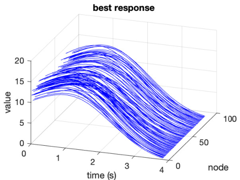
The following values will be adopted for the parameters: $\alpha=-0.5$ , $\beta=1$ , $\eta=0.1$ , $r=10$ , $T=4$ . The initial conditions $\{x_{0}^{1},x_{0}^{2}...,\}$ are chosen as independent Gaussian random variables with variance $1$ and mean $10$ .

5.1 Example on Multipartite Graphs

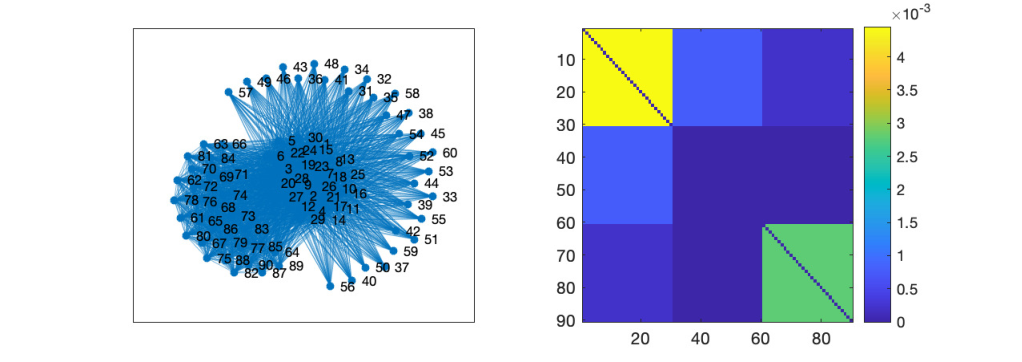
We consider multipartite graphs (with no self-loops) where the connection weights are specified by the following matrix

\begin{bmatrix}0.25&0&0.02\\ 0&0&0.07\\ 0.02&0.07&0.40\end{bmatrix}.

(40)

The sizes of the sequence of graphs are given by $3n$ where $n\in\{1,2,...\}$ is the number of nodes in each community. Since $n$ may vary, the underlying graph could be of arbitrary size. Clearly Assumptions 1(a), 4 and 5 are satisfied. Since the graphon limit has rank $3$ , Assumption 2 holds. Furthermore, the specific values for the parameters in the example allow Assumption 3 to hold. Hence, the result in Theorem 3 applies. A simulation result on a network of size $90$ is shown in Figure 2.

5.2 Example on Graphs Generated from a Sinusoidal Graphon

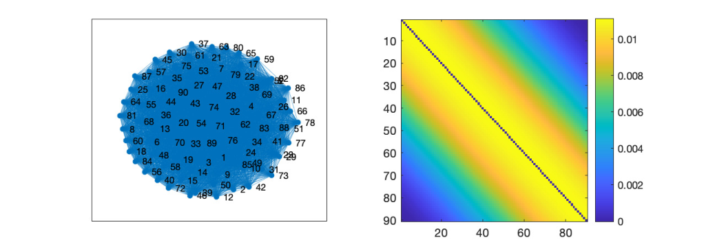
To generate a graph of size $N$ from the graphon limit $\mathbf{A}(x,y)=0.5\cos\pi(x-y)+0.5$ with $x,y\in[0,1]$ , we first get the uniform grid in $[0,1]$ with grid points $p_{1},...,p_{N}$ and then connect $i$ and $j$ ( $i\neq j$ ) with weight $\mathbf{A}(p_{i},p_{j})$ . Clearly this generation procedure ensures Assumptions 1(a), 4 and 5 are satisfied.

The normalized $L^{2}[0,1]$ eigenvectors of the graphon limit $\mathbf{A}(x,y)=0.5\cos\pi(x-y)+0.5$ associated with nonzero eigenvalues are $\mathds{1}_{[0,1]}$ , $\sqrt{2}\sin\pi(\cdot)$ and $\sqrt{2}\cos\pi(\cdot)$ , and the corresponding nonzero eigenvalue are $\frac{1}{2}$ , $\frac{1}{4}$ and $\frac{1}{4}$ (see e.g., ShuangPeterCDC19W1). Hence the graphon limit $\mathbf{A}$ has rank $3$ and Assumption 2 holds. Furthermore, the specific values for the parameters in the example allow Assumption 3 to hold. Hence, the result in Theorem 3 applies. A simulation result is shown in Figure 3.

6 Conclusions

Future work will be focused on the following LQ-GFG problem aspects: (1) LQ-GFG problems where the agent dynamics include stochastic disturbances; (2) LQ-GFG problems based on sampling procedures; (3) less restrictive conditions for the LQ-GMG $\varepsilon$ -Nash property; (4) an LQ-GFG methodology for sparse networks; (5) convergence properties of finite equilibria to the limit equilibrium; (6) general approximate solution methods to relax the finite-rank restrictions on graphon limits.

References

[1] Marco Avella-Medina, Francesca Parise, Michael Schaub, and Santiago Segarra. Centrality measures for graphons: Accounting for uncertainty in networks. IEEE Transactions on Network Science and Engineering, 2018.
[2] Alain Bensoussan, Giuseppe Da Prato, Michel C Delfour, and Sanjoy Mitter. Representation and Control of Infinite Dimensional Systems. Springer Science & Business Media, 2 edition, 2007.
[3] Alain Bensoussan, KCJ Sung, Sheung Chi Phillip Yam, and Siu-Pang Yung. Linear-quadratic mean field games. Journal of Optimization Theory and Applications, 169(2):496–529, 2016.
[4] Christian Borgs, Jennifer T Chayes, László Lovász, Vera T Sós, and Katalin Vesztergombi. Convergent sequences of dense graphs i: Subgraph frequencies, metric properties and testing. Advances in Mathematics, 219(6):1801–1851, 2008.
[5] Christian Borgs, Jennifer T Chayes, László Lovász, Vera T Sós, and Katalin Vesztergombi. Convergent sequences of dense graphs ii. multiway cuts and statistical physics. Annals of Mathematics, 176(1):151–219, 2012.
[6] Peter E. Caines and Minyi Huang. Graphon mean field games and the GMFG equations. In Proceedings of the 57th IEEE Conference on Decision and Control (CDC), pages 4129–4134, December 2018.
[7] Peter E. Caines and Minyi Huang. Graphon mean field games and the GMFG equations: $\varepsilon$ -Nash equilibria. In Proceedings of the 58th IEEE Conference on Decision and Control (CDC), pages 286–292, December 2019.
[8] Rene Carmona, Daniel Cooney, Christy Graves, and Mathieu Lauriere. Stochastic graphon games: I. the static case. arXiv preprint arXiv:1911.10664, 2019.
[9] Hayato Chiba and Georgi S Medvedev. The mean field analysis of the Kuramoto model on graphs I. the mean field equation and transition point formulas. Discrete and Continuous Dynamical Systems-Series A, 39(1):131–155, 2019.
[10] Dan Crisan, Thomas G Kurtz, and Yoonjung Lee. Conditional distributions, exchangeable particle systems, and stochastic partial differential equations. In Annales de l’IHP Probabilités et statistiques, volume 50, pages 946–974, 2014.
[11] François Delarue. Mean field games: A toy model on an Erdös-Renyi graph. ESAIM. Proceedings and Surveys, 60, 2017.
[12] T.R. Foguen, R. Malhame, and P. Caines. A quantilized mean field game approach to energy pricing with application to fleets of plug-in electric vehicles. In Proceedings of the 58th IEEE Conference on Decision and Control, pages 299–304, 2019.
[13] Shuang Gao and Peter E. Caines. The control of arbitrary size networks of linear systems via graphon limits: An initial investigation. In Proceedings of the 56th IEEE Conference on Decision and Control (CDC), pages 1052–1057, Melbourne, Australia, December 2017.
[14] Shuang Gao and Peter E. Caines. Graphon linear quadratic regulation of large-scale networks of linear systems. In Proceedings of the 57th IEEE Conference on Decision and Control (CDC), pages 5892–5897, Miami Beach, FL, USA, December 2018.
[15] Shuang Gao and Peter E. Caines. Optimal and approximate solutions to linear quadratic regulation of a class of graphon dynamical systems. In Proceedings of the 58th IEEE Conference on Decision and Control (CDC), pages 8359–8365, Nice, France, December 2019.
[16] Shuang Gao and Peter E. Caines. Spectral representations of graphons in very large network systems control. In Proceedings of the 58th IEEE Conference on Decision and Control (CDC), pages 5068–5075, Nice, France, December 2019.
[17] Shuang Gao and Peter E Caines. Graphon control of large-scale networks of linear systems. IEEE Transactions on Automatic Control, 65(10):4090–4105, 2020.
[18] Olivier Guéant. Existence and uniqueness result for mean field games with congestion effect on graphs. Applied Mathematics & Optimization, 72(2):291–303, 2015.
[19] Minyi Huang, Peter E Caines, and Roland P Malhamé. Large-population cost-coupled LQG problems with nonuniform agents: individual-mass behavior and decentralized $\varepsilon$ -nash equilibria. IEEE Transactions on Automatic Control, 52(9):1560–1571, 2007.
[20] Minyi Huang, Peter E Caines, and Roland P Malhamé. The NCE (mean field) principle with locality dependent cost interactions. IEEE Transactions on Automatic Control, 55(12):2799–2805, 2010.
[21] Minyi Huang, Peter E Caines, and Roland P Malhamé. Social optima in mean field LQG control: centralized and decentralized strategies. IEEE Transactions on Automatic Control, 57(7):1736–1751, 2012.
[22] Minyi Huang, Roland P Malhamé, and Peter E Caines. Nash equilibria for large-population linear stochastic systems of weakly coupled agents. In Analysis, control and optimization of complex dynamic systems, pages 215–252. Springer, 2005.
[23] Minyi Huang, Roland P Malhamé, and Peter E Caines. Large population stochastic dynamic games: closed-loop McKean-Vlasov systems and the Nash certainty equivalence principle. Communications in Information & Systems, 6(3):221–252, 2006.
[24] Svante Janson. Graphons, cut norm and distance, couplings and rearrangements. arXiv preprint arXiv: 1009.2376, 2010.
[25] Daniel Lacker and Agathe Soret. A case study on stochastic games on large graphs in mean field and sparse regimes. arXiv preprint arXiv:2005.14102, 2020.
[26] Jean-Michel Lasry and Pierre-Louis Lions. Jeux à champ moyen. i–le cas stationnaire. Comptes Rendus Mathématique, 343(9):619–625, 2006.
[27] Jean-Michel Lasry and Pierre-Louis Lions. Jeux à champ moyen. ii–horizon fini et contrôle optimal. Comptes Rendus Mathématique, 343(10):679–684, 2006.
[28] Frank L Lewis, Draguna Vrabie, and Vassilis L Syrmos. Optimal control. John Wiley & Sons, 2012.
[29] László Lovász. Large Networks and Graph Limits, volume 60. American Mathematical Soc., 2012.
[30] Georgi S Medvedev. The nonlinear heat equation on dense graphs and graph limits. SIAM Journal on Mathematical Analysis, 46(4):2743–2766, 2014.
[31] Georgi S Medvedev. The nonlinear heat equation on w-random graphs. Archive for Rational Mechanics and Analysis, 212(3):781–803, 2014.
[32] Francesca Parise and Asuman Ozdaglar. Graphon games. In Proceedings of the 2019 ACM Conference on Economics and Computation, pages 457–458, 2019.
[33] Julien Petit, Renaud Lambiotte, and Timoteo Carletti. Random walks on dense graphs and graphons. arXiv preprint arXiv:1909.11776, 2019.
[34] Rabih Salhab, Roland P Malhamé, and Jerome Le Ny. Collective stochastic discrete choice problems: A min-LQG dynamic game formulation. IEEE Transactions on Automatic Control, 65(8):3302–3316, 2020.
[35] Ralph Edwin Showalter. Monotone operators in Banach space and nonlinear partial differential equations, volume 49. American Mathematical Soc., 1997.
[36] H. Tembine. Quantile-based mean-field games with common noise. arXiv:1708.06035v1, 2017.

7 Appendix

7.1 Proof of Proposition 1

The proof follows immediately from the standard fixed point method and we include it here for convenience of reference.

Proof.

Consider the following transformation:

\begin{split}\tilde{z}_{t}^{\ell}&=z_{t}^{\ell}\text{exp}\left[{-\int_{0}^{t}\Big(\alpha-\frac{\beta^{2}}{r}\pi_{\tau}+\eta\lambda_{\ell}\Big)d\tau}\right]\\ \tilde{s}_{t}^{\ell}&=s_{t}^{\ell}\text{exp}\left[{-\int_{t}^{T}\Big(\alpha-\frac{\beta^{2}}{r}\pi_{\tau}\Big)d\tau}\right].\end{split}

(41)

From (16), we obtain

	$\displaystyle\dot{\tilde{z}}_{t}^{\ell}$	$\displaystyle=\frac{\beta^{2}\lambda_{\ell}}{r}\frac{1}{B_{\ell}(t)}\tilde{s}_{t}^{\ell},\quad\tilde{z}_{0}^{\ell}=z_{0}^{\ell}$		(42)
	$\displaystyle\dot{\tilde{s}}_{t}^{\ell}$	$\displaystyle=-(1-\eta\pi_{t})B_{\ell}(t)\tilde{z}_{t}^{\ell},\quad\tilde{s}_{T}^{\ell}=s_{T}^{\ell}=0$		(42)

where $B_{\ell}(t)\triangleq\text{exp}\left[{\int_{0}^{t}\Big(\alpha-\frac{\beta^{2}}{r}\pi_{\tau}+\eta\lambda_{\ell}\Big)d\tau-\int_{t}^{T}\Big(\alpha-\frac{\beta^{2}}{r}\pi_{\tau}\Big)d\tau}\right].$ Note that $B_{\ell}(t)>0$ holds for all $t\in[0,T]$ . In a compact form, we have

\begin{bmatrix}\dot{\tilde{z}}_{t}^{\ell}\\ \dot{\tilde{s}}_{t}^{\ell}\end{bmatrix}=\begin{bmatrix}0&\frac{\beta^{2}}{r}\frac{\lambda_{\ell}}{B_{\ell}(t)}\\ -(1-\eta\pi_{t})B_{\ell}(t)&0\end{bmatrix}\begin{bmatrix}\tilde{z}_{t}^{\ell}\\ \tilde{s}_{t}^{\ell}\end{bmatrix},~\begin{bmatrix}\tilde{z}_{0}^{\ell}\\ \tilde{s}_{T}^{\ell}\end{bmatrix}=\begin{bmatrix}z_{0}^{\ell}\\ s_{T}^{\ell}\end{bmatrix}.

(43)

Let $\mathbb{T}_{g}$ and $\mathbb{T}_{b}$ be linear mappings from $C([0,T];\mathds{R})$ to $C([0,T];\mathds{R})$ defined as:

	$\displaystyle\mathbb{T}_{g}(x)(t)$	$\displaystyle=z_{0}^{\ell}+\int_{0}^{t}\frac{\beta^{2}}{r}\frac{\lambda_{\ell}}{B_{\ell}(\tau)}x(\tau)d\tau,$		(44)
	$\displaystyle\mathbb{T}_{b}(x)(t)$	$\displaystyle=0+\int_{t}^{T}(1-\eta\pi_{\tau})B_{\ell}(\tau)x(\tau)d\tau,\quad t\in[0,T]$		(44)

for all $x\in C([0,T];\mathds{R})$ .

Consider the mapping $\mathbb{M}:C([0,T];\mathds{R})\rightarrow C([0,T];\mathds{R})$ defined by the composition of $\mathbb{T}_{g}$ and $\mathbb{T}_{b}$ as follows: $\mathbb{M}:x\mapsto\mathbb{T}_{g}(\mathbb{T}_{b}(x)),~x\in C([0,T];\mathds{R}).$ We consider the Banach space of continuous functions $C([0,T];\mathds{R})$ endowed with the sup norm $\|x\|_{\infty}=\sup_{t\in[0,T]}|x(t)|$ for any $x\in C([0,T];\mathds{R})$ . To show the existence of a unique fixed point to (42), we shall identify a condition for which the following holds:

\|\mathbb{M}(x)-\mathbb{M}(y)\|_{\infty}\leq L\|x-y\|_{\infty},\quad L<1.

(45)

For $t,\tau\in[0,T]$ ,

	$\displaystyle\|\mathbb{M}(x)(t)-\mathbb{M}(y)(t)\|$	$\displaystyle=\left\|\int_{0}^{t}\frac{\beta^{2}}{r}\frac{\lambda_{\ell}}{B_{\ell}(\tau)}\big(\mathbb{T}_{b}(x)(\tau)-\mathbb{T}_{b}(y)(\tau)\big)d\tau\right\|$		(46)
		$\displaystyle\leq\int_{0}^{t}\frac{\beta^{2}}{r}\frac{\|\lambda_{\ell}\|}{B_{\ell}(\tau)}\big(\big\|\mathbb{T}_{b}(x)(\tau)-\mathbb{T}_{b}(y)(\tau)\big\|\big)d\tau,$		(46)

	$\displaystyle\Big\|\mathbb{T}_{b}(x)(\tau)-\mathbb{T}_{b}(y)(\tau)\Big\|$	$\displaystyle=\left\|\int_{\tau}^{T}(1-\eta\pi_{s})B_{\ell}(s)(x(s)-y(s))ds\right\|$		(47)
		$\displaystyle\leq\int_{\tau}^{T}\left\|(1-\eta\pi_{s})\right\|B_{\ell}(s)ds\\|x-y\\|_{\infty}.$		(47)

Therefore,

\displaystyle\|\mathbb{M}(x)-\mathbb{M}(y)\|_{\infty}\leq\int_{0}^{T}\frac{\beta^{2}}{r}\frac{|\lambda_{\ell}|}{B_{\ell}(\tau)}\left(\int_{\tau}^{T}|(1-\eta\pi_{s})|B_{\ell}(s)ds\right)d\tau\|x-y\|_{\infty}.

(48)

Hence we obtain the following sufficient condition for a unique fixed point:

\int_{0}^{T}\frac{\beta^{2}}{r}\frac{|\lambda_{\ell}|}{B_{\ell}(\tau)}\int_{\tau}^{T}|(1-\eta\pi_{s})|B_{\ell}(s)dsd\tau<1.

(49)

For (15), the fixed point condition needs to be satisfied for all eigendirections. Therefore we obtain the result. ∎

7.2 Proof of Theorem 2

We define the following functions: for $t,\tau\in[0,T]$ ,

		$\displaystyle A_{c}^{N}(t)\triangleq\Big[(\alpha-\frac{\beta^{2}}{r}\pi_{t})I+\frac{\eta}{N}A_{N}\Big]$		(50)
		$\displaystyle\Phi(t,\tau)\triangleq\textup{exp}\left({\int_{\tau}^{t}A_{c}^{N}(s)ds}\right)$		(51)
		$\displaystyle\Gamma(t,\tau)\triangleq\textup{exp}\left({\int_{\tau}^{t}(\alpha-\frac{\beta^{2}}{r}\pi_{s})ds}\right).$		(52)

Clearly $\Phi(t,\tau)=\Gamma(t,\tau)\text{exp}\left(\frac{\eta(t-\tau)}{N}A_{N}\right),$ where the first part $\Gamma(t,\tau)$ is just a scalar and the second part $\text{exp}\left(\frac{\eta(t-\tau)}{N}A_{N}\right)$ is a $N\times N$ matrix. The same definitions are also used in Appendix section 8.1.

Proof.

Let $\mathbf{z}^{\gamma}_{t}\triangleq\sum_{\ell=1}^{d}z^{\ell}_{t}\mathbf{f}_{\ell}(\gamma),~\gamma\in[0,1],$ be the local graphon field calculated based on (26) and $\mathbf{z}^{\gamma}$ denote its trajectory over time $[0,T]$ . Denote the $N$ -uniform partition of $[0,1]$ by $\{P_{1},...,P_{N}\}$ . For $P_{i}\subset[0,1]$ , let

\displaystyle\bar{\mathbf{z}}^{i}_{t}

\displaystyle\triangleq\frac{1}{\mu(P_{i})}\int_{P_{i}}\mathbf{z}^{\gamma}_{t}d\gamma\in\mathds{R}\quad\text{and}\quad\bar{\mathbf{z}}_{t}^{\gamma}\triangleq\bar{\mathbf{z}}_{t}^{i},~\gamma\in P_{i}

Their trajectories over time $[0,T]$ are respectively denoted by $\bar{\mathbf{z}}^{i}$ and $\bar{\mathbf{z}}$ . Similarly we define $\bar{\mathbf{s}}_{t}$ , $\bar{\mathbf{s}}_{t}^{i}$ , $\bar{\mathbf{s}}$ and $\bar{\mathbf{s}}^{i}$ .

For agent $i$ corresponding to $P_{i}\subset[0,1]$ , the cost induced by following the infinite population and graphon limit Nash law in Strategy 1 is given by

		$\displaystyle J({u}^{oi},u^{-oi})=\frac{1}{2}\int_{0}^{T}\Big((x^{oi}_{t}-\frac{1}{N}\sum_{j=1}^{N}a_{ij}x^{oj}_{t})^{2}+r(u_{t}^{oi})^{2}\Big)dt$
		$\displaystyle=J({u}^{oi},\bar{\mathbf{z}}^{i})+\frac{1}{2}\int_{0}^{T}\Big[(\bar{\mathbf{z}}_{t}^{i}-\frac{1}{N}\sum_{j=1}^{N}a_{ij}x^{oj}_{t})\Big]^{2}_{({u}^{oi},u^{-oi})}dt$
		$\displaystyle+\int_{0}^{T}\Big[(x^{oi}_{t}-\bar{\mathbf{z}}_{t}^{i})(\bar{\mathbf{z}}_{t}^{i}-\frac{1}{N}\sum_{j=1}^{N}a_{ij}x^{oj}_{t})\Big]_{({u}^{oi},u^{-oi})}dt$
		$\displaystyle\triangleq J({u}^{oi},\bar{\mathbf{z}}^{i})+\frac{1}{2}I_{2}+\frac{1}{2}I_{3},$

where $x_{t}^{oi}$ and $u_{t}^{oi}$ represent respectively the state and the action for agent $i$ at time $t$ under the prescribed $\varepsilon$ -Nash law. We use $(u^{oi},u^{-oi})$ in the subscript to indicate the underlying strategy. By the Cauchy-Schwarz inequality, we obtain

\displaystyle|I_{3}|

\displaystyle\leq 2\sqrt{I_{2}}\left[\int_{0}^{T}(x^{oi}_{t}-\bar{\mathbf{z}}_{t}^{i})^{2}dt\right]^{\frac{1}{2}}_{({u}^{oi},u^{-oi})}.

(53)

Similarly, we obtain

		$\displaystyle J({u}^{i},u^{-oi})=\frac{1}{2}\int_{0}^{T}\Big((x^{i}_{t}-\frac{1}{N}\sum_{j=1}^{N}a_{ij}x^{j}_{t})^{2}+r(u_{t}^{i})^{2}\Big)_{({u}^{i},u^{-oi})}dt$
		$\displaystyle=\frac{1}{2}\int_{0}^{T}\Big[(x^{i}_{t}-\bar{\mathbf{z}}_{t}^{i})^{2}+r(u_{t}^{i})^{2}\Big]dt+\frac{1}{2}\int_{0}^{T}\Big[(\bar{\mathbf{z}}_{t}^{i}-\frac{1}{N}\sum_{j=1}^{N}a_{ij}x^{j}_{t})\Big]^{2}_{({u}^{i},u^{-oi})}dt$
		$\displaystyle+\int_{0}^{T}\Big[(x^{i}_{t}-\bar{\mathbf{z}}_{t}^{i})(\bar{\mathbf{z}}_{t}^{i}-\frac{1}{N}\sum_{j=1}^{N}a_{ij}x^{j}_{t})\Big]_{({u}^{i},u^{-oi})}dt$
		$\displaystyle\triangleq J(u^{i},\bar{\mathbf{z}}^{i})+\frac{1}{2}I^{\prime}_{2}+\frac{1}{2}I^{\prime}_{3}.$

and

\displaystyle|I^{\prime}_{3}|

\displaystyle\leq 2\sqrt{I^{\prime}_{2}}\left[\int_{0}^{T}(x^{i}_{t}-\bar{\mathbf{z}}_{t}^{i})^{2}dt\right]^{\frac{1}{2}}_{({u}^{i},u^{-oi})}.

(54)

Therefore, we obtain the following:

		$\displaystyle J(u^{oi},u^{-oi})-J(u^{i},u^{-oi})$		(55)
		$\displaystyle=J(u^{oi},u^{-oi})-J(u^{oi},\bar{\mathbf{z}}^{i})+J(u^{oi},\bar{\mathbf{z}}^{i})-J(u^{i},\bar{\mathbf{z}}^{i})+J(u^{i},\bar{\mathbf{z}}^{i})-J(u^{i},u^{-oi})$
		$\displaystyle{\displaystyle\leq}\frac{1}{2}(\|I_{2}\|+\|I_{3}\|)+\|\left(J(u^{oi},\bar{\mathbf{z}}^{i})-J(u^{i},\bar{\mathbf{z}}^{i})\right)\|+\frac{1}{2}(\|I_{2}^{\prime}\|+\|I_{3}^{\prime}\|).$

We will establish the following asymptotic estimates for $I_{2}$ , $I_{3}$ , $I_{2}^{\prime}$ and $I_{3}^{\prime}$ : for fixed $T>0$ ,

		$\displaystyle\|I_{2}\|=O\Big(E_{N}^{2}\Big),\quad\|I_{3}\|=\max\left\{O\Big(E_{N}\Big),O\Big(E_{N}^{2}\Big)\right\},$		(56)
		$\displaystyle\|I_{2}^{\prime}\|=O\Big(E_{N}^{2}\Big),\quad\|I_{3}^{\prime}\|=\max\left\{O\Big(E_{N}\Big),O\Big(E_{N}^{2}\Big)\right\},$		(56)

where $E_{N}\triangleq\max_{1\leq i\leq N}\frac{1}{\mu(P_{i})}\left\|(\mathbf{A}-\mathbf{A}^{\mathbf{N}})\mathds{1}_{P_{i}}\right\|_{2}.$ These estimates, together with Lemma 1 and (55), imply that

\displaystyle J(u^{oi},u^{-oi})-\inf_{u^{i}\in\mathcal{U}}J(u^{i},u^{-oi})=\max\left\{O(E_{N}),O(E_{N}^{2})\right\}.

(57)

The rest of the proof will be devoted to establishing the asymptotic estimates for $I_{2}$ , $I_{3}$ , $I_{2}^{\prime}$ and $I_{3}^{\prime}$ .

1) Estimate for $I_{2}$

The next step is to show the upper bound for the term $I_{2}$ :

\displaystyle I_{2}

\displaystyle\triangleq\int_{0}^{T}\Big[(\bar{\mathbf{z}}_{t}^{i}-\frac{1}{N}\sum_{j=1}^{N}a_{ij}x^{oj}_{t})\Big]^{2}_{({u}^{oi},u^{-oi})}dt.

(58)

Based on (15), we obtain

$\displaystyle\dot{\bar{\mathbf{z}}}_{t}^{i}$	$\displaystyle=\Big(\alpha-\frac{\beta^{2}}{r}\pi_{t}\Big)\bar{\mathbf{z}}_{t}^{i}+\eta\frac{1}{\mu(P_{i})}\int_{P_{i}}[\mathbf{A}\mathbf{z}_{t}]^{\gamma}d\gamma$	(59)
	$\displaystyle~~+\frac{\beta^{2}}{r}\frac{1}{\mu(P_{i})}\int_{P_{i}}[\mathbf{A}\mathbf{s}_{t}]^{\gamma}d\gamma,~\bar{\mathbf{z}}_{0}^{i}=\frac{1}{\mu(P_{i})}\int_{P_{i}}[\mathbf{A}\mathbf{x}_{0}^{\mathbf{N}}]^{\gamma}d\gamma,$
$\displaystyle\dot{\mathbf{s}}_{t}^{i}$	$\displaystyle=-\Big(\alpha-\frac{\beta^{2}}{r}\pi_{t}\Big)\bar{\mathbf{s}}_{t}^{i}-(1-\eta\pi_{t})\bar{\mathbf{z}}_{t}^{i},\quad\bar{\mathbf{s}}^{i}_{T}=0.$	(60)

The closed loop dynamics for the $i$ th agent under Strategy 1 in the finite population problem is given by

\displaystyle\dot{x}_{t}^{oi}

\displaystyle=\Big(\alpha-\frac{\beta^{2}}{r}\pi_{t}\Big){x}^{oi}_{t}+\eta\frac{1}{N}\sum_{j=1}^{N}a_{ij}x^{oj}_{t}+\frac{\beta^{2}}{r}\bar{\mathbf{s}}_{t}^{i}.

(61)

Let ${\mathbf{z}}_{t}^{o\mathbf{N}}\in L^{2}[0,1]$ denote the step function that corresponds to the vector $[z_{t}^{o1}\ldots z_{t}^{oN}]^{\mathchoice{\raisebox{0.0pt}{$\displaystyle\intercal$}}{\raisebox{0.0pt}{$\textstyle\intercal$}}{\raisebox{0.0pt}{$\scriptstyle\intercal$}}{\raisebox{0.0pt}{$\scriptscriptstyle\intercal$}}}$ . Let $\Delta_{t}^{Ni}\triangleq\bar{\mathbf{z}}_{t}^{i}-z_{t}^{oi}.$ Then

	$\displaystyle\dot{\Delta}_{t}^{Ni}=$	$\displaystyle\Big(\alpha-\frac{\beta^{2}}{r}\pi_{t}\Big)\Delta_{t}^{Ni}+\frac{\beta^{2}}{r}\frac{1}{\mu(P_{i})}\int_{P_{i}}\Big[\mathbf{A}\mathbf{s}_{t}-\mathbf{A}^{\mathbf{N}}\bar{\mathbf{s}}_{t}\Big]^{\gamma}d\gamma,$
		$\displaystyle+\eta\frac{1}{\mu(P_{i})}\int_{P_{i}}\big[\mathbf{A}\mathbf{z}_{t}-\mathbf{A}^{\mathbf{N}}\mathbf{z}_{t}^{o\mathbf{N}}\big]^{\gamma}d\gamma$
	$\displaystyle=$	$\displaystyle\Big(\alpha-\frac{\beta^{2}}{r}\pi_{t}\Big)\Delta_{t}^{Ni}+\frac{\beta^{2}}{r}\frac{1}{\mu(P_{i})}\Big\langle\mathds{1}_{P_{i}},(\mathbf{A}-\mathbf{A}^{\mathbf{N}})\mathbf{s}_{t}\Big\rangle$
		$\displaystyle+\eta\frac{1}{\mu(P_{i})}\left\langle\mathds{1}_{P_{i}},(\mathbf{A}-\mathbf{A}^{\mathbf{N}})\mathbf{z}_{t}\right\rangle+\eta\frac{1}{N}\sum_{j=1}^{N}a_{ij}\Delta_{t}^{Nj}.$

Therefore,

\displaystyle\dot{\Delta}_{t}^{N}=\Big[(\alpha-\frac{\beta^{2}}{r}\pi_{t})I+\frac{\eta}{N}A_{N}\Big]{\Delta}_{t}^{N}+\frac{\beta^{2}}{r}D_{t}^{N\mathbf{s}}+\eta D_{t}^{N\mathbf{z}}

(62)

where

	$\displaystyle D_{t}^{N\mathbf{s}}$	$\displaystyle=\left(\frac{1}{\mu(P_{i})}\Big\langle\mathds{1}_{P_{i}},(\mathbf{A}-\mathbf{A}^{\mathbf{N}})\mathbf{s}_{t}\Big\rangle\right)_{i=1}^{N}\in\mathds{R}^{N},$
	$\displaystyle D_{t}^{N\mathbf{z}}$	$\displaystyle=\left(\frac{1}{\mu(P_{i})}\Big\langle\mathds{1}_{P_{i}},(\mathbf{A}-\mathbf{A}^{\mathbf{N}})\mathbf{z}_{t}\Big\rangle\right)_{i=1}^{N}\in\mathds{R}^{N}.$

The initial condition is given by $\Delta_{0}^{N}=[\Delta_{0}^{N1},\ldots,\Delta_{0}^{NN}]^{\mathchoice{\raisebox{0.0pt}{$\displaystyle\intercal$}}{\raisebox{0.0pt}{$\textstyle\intercal$}}{\raisebox{0.0pt}{$\scriptstyle\intercal$}}{\raisebox{0.0pt}{$\scriptscriptstyle\intercal$}}}$ where

\displaystyle\Delta_{0}^{Ni}

\displaystyle=\bar{\mathbf{z}}_{0}^{i}-z_{0}^{oi}=\frac{1}{\mu{(P_{i})}}\big\langle\mathds{1}_{P_{i}},(\mathbf{A}-\mathbf{A}^{\mathbf{N}})\mathbf{x}_{0}^{\mathbf{N}}\big\rangle.

(63)

We want to ensure that $\|\Delta_{t}^{N}\|_{\infty}\triangleq\max_{i}\{|\Delta_{t}^{Ni}|\}$ is bounded and establish the rate of convergence with respect to $N$ . The solution $\{\Delta_{t}^{N},t\in[0,T]\}$ to (62) with the initial condition specified by (63) is given as follows:

\Delta_{t}^{N}=\Phi(t,0)\Delta_{0}^{N}+\int_{0}^{t}\Phi(t,\tau)\Big(\frac{\beta^{2}}{r}D_{\tau}^{N\mathbf{s}}+\eta D_{t}^{N\mathbf{z}}\Big)d\tau.

(64)

By the definition of $\|\cdot\|_{\infty}$ , we obtain

	$\displaystyle\\|\Delta_{t}^{N}\\|_{\infty}$	$\displaystyle\leq\left\\|\Phi(t,0)\right\\|_{\infty}\\|\Delta_{0}^{N}\\|_{\infty}+\int_{0}^{t}\left\\|\Phi(t,\tau)\Big(\frac{\beta^{2}}{r}D_{\tau}^{N\mathbf{s}}+\eta D_{\tau}^{N\mathbf{z}}\Big)\right\\|_{\infty}d\tau$		(65)
		$\displaystyle\leq\Big\\|\Phi(t,0)\Big\\|_{\infty}E_{N}\\|\mathbf{x}_{0}^{\mathbf{N}}\\|_{2}+\int_{0}^{t}\left\\|\Phi(t,\tau)\right\\|_{\infty}E_{N}\Big(\frac{\beta^{2}}{r}\\|\mathbf{s}_{\tau}\\|_{2}+\|\eta\|\\|\mathbf{z}_{\tau}\\|_{2}\Big)d\tau$		(65)

where $E_{N}\triangleq\max_{1\leq i\leq N}\frac{1}{\mu(P_{i})}\left\|(\mathbf{A}-\mathbf{A}^{\mathbf{N}})\mathds{1}_{P_{i}}\right\|_{2}.$ Furthermore, $\left\|\Phi(t,\tau)\right\|_{\infty}$ with $t\geq\tau$ is uniformly bounded in $N$ since

\displaystyle\left\|\Phi(t,\tau)\right\|_{\infty}

\displaystyle=\Gamma(t,\tau)\left\|e^{(t-\tau)\frac{\eta}{N}A}\right\|_{\infty}\leq\Gamma(t,\tau)e^{(t-\tau)|\eta|c}

(66)

where $|a_{ij}|\leq c$ as in Assumption 4. Since $\left\|\Phi(t,\tau)\right\|_{\infty}$ , $\|\mathbf{x}_{0}^{\mathbf{N}}\|_{2}$ , $\|\mathbf{s}_{\tau}\|_{2}$ and $\|\mathbf{z}_{\tau}\|_{2}$ are all uniformly bounded in $N$ , (65) implies

\|\Delta_{t}^{N}\|_{\infty}=O\Big(E_{N}\Big).

(67)

Hence, by the definition of $I_{2}$ , for fixed $T>0$ ,

|I_{2}|=O\Big(E_{N}^{2}\Big).

(68)

2) Estimate for $I_{3}$

Similarly, letting $\delta_{t}^{Ni}\triangleq\bar{\mathbf{z}}^{i}_{t}-x_{t}^{oi}$ we obtain

$\displaystyle\dot{\delta}_{t}^{Ni}=$	$\displaystyle(\alpha-\frac{\beta^{2}}{r}\pi_{t})\delta_{t}^{Ni}+\frac{\beta^{2}}{r}\left[\frac{1}{\mu(P_{i})}\int_{P_{i}}\big[\mathbf{A}\mathbf{s}_{t}\big]^{\gamma}d\gamma-\bar{\mathbf{s}}_{t}^{i}\right]$	(69)
	$\displaystyle+\eta\left[\frac{1}{\mu(P_{i})}\int_{P_{i}}[\mathbf{A}\mathbf{z}_{t}]^{\gamma}d\gamma-\frac{1}{N}\sum_{j=1}^{N}a_{ij}x^{oj}_{t}\right]$
$\displaystyle=$	$\displaystyle(\alpha-\frac{\beta^{2}}{r}\pi_{t})\delta_{t}^{Ni}+\frac{\beta^{2}}{r}\frac{1}{\mu(P_{i})}\langle(\mathbf{A}-\mathbb{I})\mathds{1}_{P_{i}},\mathbf{s}_{t}\rangle$
	$\displaystyle+\eta\frac{1}{\mu(P_{i})}\langle(\mathbf{A}-\mathbb{I})\mathds{1}_{P_{i}},\mathbf{z}_{t}\rangle+\eta\Delta_{t}^{Ni}.$

Therefore,

	$\displaystyle\delta_{t}^{Ni}$	$\displaystyle=\Gamma(t,0)\delta_{0}^{Ni}+\int_{0}^{t}\Gamma(t,\tau)\frac{\beta^{2}}{r}\frac{1}{\mu(P_{i})}\langle(\mathbf{A}-\mathbb{I})\mathds{1}_{P_{i}},\mathbf{s}_{\tau}\rangle d\tau$
		$\displaystyle+\int_{0}^{t}\Gamma(t,\tau)\frac{\eta}{\mu(P_{i})}\langle(\mathbf{A}-\mathbb{I})\mathds{1}_{P_{i}},\mathbf{z}_{\tau}\rangle d\tau+\int_{0}^{t}\Gamma(t,\tau)\eta\Delta_{\tau}^{Ni}d\tau$
		$\displaystyle\leq\Gamma(t,0)\\|\mathbf{A}-\mathbb{I}\\|_{\text{op}}\\|\mathbf{x}_{0}^{\mathbf{N}}\\|_{2}$
		$\displaystyle+\int_{0}^{t}\Gamma(t,\tau)\\|(\mathbf{A}-\mathbb{I})\\|_{\text{op}}\Big(\frac{\beta^{2}}{r}\\|\mathbf{s}_{\tau}\\|_{2}+\eta\\|\mathbf{z}_{\tau}\\|_{2}\Big)d\tau+\int_{0}^{t}\Gamma(t,\tau)\eta\Delta_{\tau}^{Ni}d\tau$

with the initial condition

\displaystyle\delta_{0}^{Ni}

\displaystyle=\bar{\mathbf{z}}^{i}_{0}-x_{0}^{oi}=\frac{1}{\mu(P_{i})}\langle(\mathbf{A}-\mathbb{I})\mathds{1}_{P_{i}},\mathbf{x}_{0}^{\mathbf{N}}\rangle.

Furthermore, since $\mathbf{x}_{0}^{\mathbf{N}}$ , $\mathbf{z}_{t}$ , $\mathbf{s}_{t}$ , $\mathbf{A}$ , $\|\mathbf{A}-\mathbb{I}\|_{\text{op}}$ are uniformly bounded in $N$ and $\Delta_{t}^{Ni}$ is of the order $E_{N}$ for all $i$ , we obtain $|\delta_{t}^{Ni}|=\max\left\{O(1),O(E_{N})\right\}.$ This together with (53) and (68) implies

|I_{3}|=\max\left\{O\Big(E_{N}\Big),O\Big(E_{N}^{2}\Big)\right\}.

(70)

3) Estimates for $I_{2}^{\prime}$ and $I_{3}^{\prime}$

By Assumption 4, $I_{2}^{\prime}=I_{2}$ . Thus

|I_{2}^{\prime}|=O(E_{N}^{2})

(71)

Similar to (70), we obtain

|I_{3}^{\prime}|=\max\left\{O(E_{N}),O(E_{N}^{2})\right\}.

(72)

∎

Lemma for Theorem 2

Let $x^{oi},i\in\{1,...,N\}$ , denotes the state trajectory of agent $j$ when all agents are following Strategy 1. Assume the following trajectories are given to an arbitrary agent indexed by $i$ :

•

the reference trajectory $\bar{\mathbf{z}}^{i}_{t}\triangleq\frac{1}{\mu(P_{i})}\int_{P_{i}}\mathbf{z}^{\gamma}_{t}d\gamma$ for all $t\in[0,T]$ with $\mathbf{z}$ as the graphon filed of the corresponding limit graphon field game problem satisfying (15)
•

the dynamic offset $z_{t}^{oi}\triangleq\frac{1}{N}\sum_{j\in\mathcal{N}_{i}}a_{ij}x_{t}^{oj}$ for all $t\in[0,T]$ where $\mathcal{N}_{i}$ denotes the set of neighours for agent $i$ excluding itself.

Then consider the following linear quadratic tracking problem for agent $i$ :

		$\displaystyle\dot{x}_{t}^{i}=\alpha x_{t}^{i}+\beta u_{t}^{i}+\eta\frac{1}{N}\sum_{j\in\mathcal{N}_{i}}a_{ij}x_{t}^{oj}$		(73)
		$\displaystyle J(u^{i},\bar{\mathbf{z}}^{i})=\frac{1}{2}\int_{0}^{T}\left[(x^{i}_{t}-\bar{\mathbf{z}}_{t}^{i})^{2}+r(u_{t}^{i})^{2}\right]dt.$		(73)

Lemma 1.

Under Assumptions 1, 2, 3 and 4, the following estimate for the difference between costs based on different control laws for the problem in (73) holds

J(u^{oi},\bar{\mathbf{z}}^{i})-\inf_{u^{i}\in\mathcal{U}}J(u^{i},\bar{\mathbf{z}}^{i})=O\Big(E_{N}\Big),

(74)

where $u^{oi}$ is generated based on Strategy 1, $\mathcal{U}\triangleq L^{2}([0,T];\mathds{R})$ and $E_{N}\triangleq\max_{1\leq i\leq N}\frac{1}{\mu(P_{i})}\left\|(\mathbf{A}-\mathbf{A}^{\mathbf{N}})\mathds{1}_{P_{i}}\right\|_{2}$ .

Proof.

The optimal control law for the problem (73) is given by

$\displaystyle u_{t}^{*i}$	$\displaystyle=-\frac{\beta}{r}\pi_{t}x_{t}^{i}+\frac{\beta}{r}s_{t}^{i},$	(75)
$\displaystyle-\dot{\pi}_{t}$	$\displaystyle=2\alpha\pi_{t}-\frac{\beta^{2}}{r}\pi_{t}^{2}+1,\qquad\pi_{T}=0,$	(76)
$\displaystyle-\dot{s}_{t}^{*i}$	$\displaystyle=\Big(\alpha-\frac{\beta^{2}}{r}\pi_{t}\Big)s_{t}^{i}+\bar{\mathbf{z}}_{t}^{i}-\eta\pi_{t}z_{t}^{oi},\quad s_{T}^{i}=0,$	(77)

The dynamics and cost under the optimal control are respectively given by

		$\displaystyle\dot{x}_{t}^{i}=\alpha x_{t}^{i}+\beta u_{t}^{*i}+\eta\frac{1}{N}\sum_{j\in\mathcal{N}_{i}}a_{ij}x_{t}^{oj}$		(78)
		$\displaystyle J(u^{i},\bar{\mathbf{z}}^{i})=\frac{1}{2}\int_{0}^{T}\left[(x^{i}_{t}-\bar{\mathbf{z}}_{t}^{i})^{2}+r(u_{t}^{*i})^{2}\right]dt.$		(79)

On the other hand, the control following Strategy 1 is given by

{u}^{oi}_{t}=-\frac{\beta}{r}\pi_{t}x_{t}^{oi}+\frac{\beta}{r}\bar{\mathbf{s}}_{t}^{i}

(80)

with $\bar{\mathbf{s}}^{i}$ defined as in (27) and $\pi_{(\cdot)}$ given by (76). Assumptions 1, 2 and 3 ensure that $\bar{\mathbf{s}}^{i}$ always exists. The associated dynamics and cost for agent $i$ are then respectively given by

		$\displaystyle\dot{x}_{t}^{oi}=\alpha x_{t}^{oi}+\beta u_{t}^{oi}+\eta\frac{1}{N}\sum_{j\in\mathcal{N}_{i}}a_{ij}x_{t}^{oj}$		(81)
		$\displaystyle J(u^{oi},\bar{\mathbf{z}}^{i})=\frac{1}{2}\int_{0}^{T}\left[(x^{oi}_{t}-\bar{\mathbf{z}}_{t}^{i})^{2}+r(u_{t}^{oi})^{2}\right]dt.$		(82)

Based on the definition of $\bar{\mathbf{s}}_{t}^{i}$ in (27) and that of $\bar{\mathbf{z}}_{t}^{i}$ , it is obvious that

\displaystyle\dot{\bar{\mathbf{s}}}_{t}^{i}

\displaystyle=-\Big(\alpha-\frac{\beta^{2}}{r}\pi_{t}\Big)\bar{\mathbf{s}}_{t}^{i}-(1-\eta\pi_{t})\bar{\mathbf{z}}_{t}^{i},\quad\bar{\mathbf{s}}^{i}_{T}=0.

(83)

This together with (77) yields

\frac{d(\bar{\mathbf{s}}_{t}^{i}-s_{t}^{*i})}{dt}=-\Big(\alpha-\frac{\beta^{2}}{r}\pi_{t}\Big)(\bar{\mathbf{s}}_{t}^{i}-s_{t}^{*i})+\eta\pi_{t}(\bar{\mathbf{z}}_{t}^{i}-z_{t}^{oi}).

(84)

Let $\Delta_{t}^{Ni}\triangleq\bar{\mathbf{z}}_{t}^{i}-z_{t}^{oi}.$ Then $(\bar{\mathbf{s}}_{t}^{i}-s_{t}^{*i})=\int_{T}^{t}\Gamma(t,\tau)\eta\pi_{\tau}\Delta_{\tau}^{Ni}d\tau$ and

(\bar{\mathbf{s}}_{t}^{i}-s_{t}^{*i})=O\Big(E_{N}\Big),\quad i\in\{1,...,N\}.

(85)

By comparing the following closed-loop dynamics under these two different control laws, we obtain

\displaystyle\frac{d(x_{t}^{oi}-x_{t}^{*i})}{dt}

\displaystyle=\Big(\alpha-\frac{\beta^{2}}{r}\pi_{t}\Big)(x_{t}^{oi}-x_{t}^{*i})+\frac{\beta^{2}}{r}(\bar{\mathbf{s}}_{t}^{i}-s^{*i}_{t}),~x_{0}^{oi}-x_{0}^{*i}=0.

Therefore, the difference is explicitly obtained as

\displaystyle x_{t}^{oi}-x_{t}^{*i}

\displaystyle=\frac{\eta\beta^{2}}{r}\int_{0}^{t}\Gamma(t,\tau)\left(\int_{T}^{\tau}\Gamma(\tau,q)\eta\pi_{q}\Delta_{q}^{Ni}dq\right)d\tau.

(86)

Under Assumption 4, $\sum_{j=1}^{N}a_{ij}x^{oj}=\sum_{j\in\mathcal{N}_{i}}a_{ij}x^{oj}$ for all $i\in\{1,\ldots,N\}$ . Then the result from (67) applies here, that is, $\forall t\in[0,T],~|\Delta_{t}^{Ni}|=O\Big(E_{N}\Big).$ Hence for any $t\in[0,T]$ , $|(x_{t}^{oi}-x_{t}^{*i})|=O\Big(E_{N}\Big).$ This, together with (85), implies $|(u_{t}^{oi}-u_{t}^{*i})|=O\Big(E_{N}\Big).$ Hence $\left|J(u^{oi},\bar{\mathbf{z}}^{i})-J(u^{*i},\bar{\mathbf{z}}^{i})\right|=O\Big(E_{N}\Big),$ that is, we obtain (74).

∎

8 Appendix II

8.1 Proof of Theorem 3

Proof.

Let $\mathbf{z}^{\gamma}_{t}\triangleq\sum_{\ell=1}^{d}z^{\ell}_{t}\mathbf{f}_{\ell}(\gamma),~\gamma\in[\underline{\gamma},\overline{\gamma}]\subset[0,1],$ be the Local Graphon Field calculated based on Strategy 2 and $\mathbf{z}^{\gamma}$ denote its trajectory over time $[0,T]$ . For $P_{i}\subset[0,1]$ , let $\bar{\mathbf{z}}^{i}_{t}\triangleq\frac{1}{\mu(P_{i})}\int_{P_{i}}\mathbf{z}^{\gamma}_{t}d\gamma$ and $\bar{\mathbf{z}}_{t}^{\gamma}\triangleq\bar{\mathbf{z}}_{t}^{i},~\gamma\in P_{i}.$ Let $\bar{\mathbf{z}}^{i}$ and $\bar{\mathbf{z}}$ respectively denote their trajectories over time $[0,T]$ . Similarly we define $\bar{\mathbf{s}}_{t}$ , $\bar{\mathbf{s}}_{t}^{i}$ , $\bar{\mathbf{s}}$ and $\bar{\mathbf{s}}^{i}$ .

For agent $i$ that corresponds to $P_{i}\subset[0,1]$ , the cost induced by following the limit control law is given by

		$\displaystyle J({u}^{oi},u^{-oi})=\frac{1}{2}\mathds{E}\int_{0}^{T}\Big((x^{oi}_{t}-\frac{1}{N}\sum_{j=1}^{N}a_{ij}x^{oj}_{t})^{2}+r(u_{t}^{oi})^{2}\Big)dt$
		$\displaystyle=J({u}^{oi},\bar{\mathbf{z}}^{i})+\frac{1}{2}\mathds{E}\int_{0}^{T}\Big[(\bar{\mathbf{z}}_{t}^{i}-\frac{1}{N}\sum_{j=1}^{N}a_{ij}x^{oj}_{t})\Big]^{2}_{({u}^{oi},u^{-oi})}dt$
		$\displaystyle+\mathds{E}\int_{0}^{T}\Big[(x^{oi}_{t}-\bar{\mathbf{z}}_{t}^{i})(\bar{\mathbf{z}}_{t}^{i}-\frac{1}{N}\sum_{j=1}^{N}a_{ij}x^{oj}_{t})\Big]_{({u}^{oi},u^{-oi})}dt$
		$\displaystyle\triangleq J({u}^{oi},\bar{\mathbf{z}}^{i})+\frac{1}{2}I_{2}+\frac{1}{2}I_{3},$

where $x_{t}^{oi}$ and $u_{t}^{oi}$ represent respectively the state and control for agent $i$ at time $t$ under the prescribed $\varepsilon$ -Nash law. By the Cauchy-Schwarz inequality, we obtain

\displaystyle I_{3}

\displaystyle\leq 2\sqrt{I_{2}}\left[\mathds{E}\int_{0}^{T}(x^{oi}_{t}-\bar{\mathbf{z}}_{t}^{i})^{2}dt\right]^{\frac{1}{2}}_{({u}^{oi},u^{-oi})}.

(87)

Let $J({u}^{i},u^{-oi})$ denote the cost for agent $i$ by unilaterally deviating from the prescribed $\varepsilon$ -Nash law where all other agents following the prescribed $\varepsilon$ -Nash law. Then

	$\displaystyle J({u}^{i},u^{-oi})$	$\displaystyle=\frac{1}{2}\mathds{E}\int_{0}^{T}\Big((x^{i}_{t}-\frac{1}{N}\sum_{j=1}^{N}a_{ij}x^{j}_{t})^{2}+r(u_{t}^{i})^{2}\Big)_{({u}^{i},u^{-oi})}dt$
		$\displaystyle=J(u^{i},\bar{\mathbf{z}}^{i})+\frac{1}{2}\mathds{E}\int_{0}^{T}\Big[(\bar{\mathbf{z}}_{t}^{i}-\frac{1}{N}\sum_{j=1}^{N}a_{ij}x^{j}_{t})\Big]^{2}_{({u}^{i},u^{-oi})}dt$
		$\displaystyle+\mathds{E}\int_{0}^{T}\Big[(x^{i}_{t}-\bar{\mathbf{z}}_{t}^{i})(\bar{\mathbf{z}}_{t}^{i}-\frac{1}{N}\sum_{j=1}^{N}a_{ij}x^{j}_{t})\Big]_{({u}^{i},u^{-oi})}dt$
		$\displaystyle\triangleq J(u^{i},\bar{\mathbf{z}}^{i})+\frac{1}{2}I^{\prime}_{2}+\frac{1}{2}I^{\prime}_{3}.$

Similarly,

\displaystyle|I^{\prime}_{3}|

\displaystyle\leq 2\sqrt{I^{\prime}_{2}}\left[\mathds{E}\int_{0}^{T}(x^{i}_{t}-\bar{\mathbf{z}}_{t}^{i})^{2}dt\right]^{\frac{1}{2}}_{({u}^{i},u^{-oi})}.

(88)

Therefore, we obtain the following:

		$\displaystyle J(u^{oi},u^{-oi})-J(u^{i},u^{-oi})$		(89)
		$\displaystyle=J(u^{oi},u^{-oi})-J(u^{oi},\bar{\mathbf{z}}^{i})+J(u^{oi},\bar{\mathbf{z}}^{i})-J(u^{i},\bar{\mathbf{z}}^{i})+J(u^{i},\bar{\mathbf{z}}^{i})-J(u^{i},u^{-oi})$
		$\displaystyle{\displaystyle\leq}\frac{1}{2}(\|I_{2}\|+\|I_{3}\|)+\|\left(J(u^{oi},\bar{\mathbf{z}}^{i})-J(u^{i},\bar{\mathbf{z}}^{i})\right)\|+\frac{1}{2}(\|I_{2}^{\prime}\|+\|I_{3}^{\prime}\|).$

We will establish the following asymptotic estimates for $I_{2}$ , $I_{3}$ , $I_{2}^{\prime}$ and $I_{3}^{\prime}$ : for fixed $T>0$ , for any $i\in\{1,...,N\}$ ,

		$\displaystyle\|I_{2}\|=\max\Big\{O\Big(\frac{1}{N}\Big),O(E_{N}^{2})\Big\},\quad\|I_{3}\|=\max\left\{O\Big(\frac{1}{\sqrt{N}}\Big),O\Big(E_{N}\Big),O\Big(E_{N}^{2}\Big)\right\},$		(90)
		$\displaystyle\|I_{2}^{\prime}\|=\max\Big\{O\Big(\frac{1}{N}\Big),O(E_{N}^{2})\Big\},\quad\|I_{3}^{\prime}\|=\max\left\{O\Big(\frac{1}{\sqrt{N}}\Big),O\Big(E_{N}\Big),O\Big(E_{N}^{2}\Big)\right\},$		(90)

where $E_{N}\triangleq\max_{1\leq i\leq N}\frac{1}{\mu(P_{i})}\left\|(\mathbf{A}-\mathbf{A}^{\mathbf{N}})\mathds{1}_{P_{i}}\right\|_{2}.$ These estimates, together with Lemma 2 and (89), imply that

\displaystyle J(u^{oi},u^{-oi})-\inf_{u^{i}\in\mathcal{U}}J(u^{i},u^{-oi})=\max\left\{O\Big(\frac{1}{\sqrt{N}}\Big),O\Big(E_{N}\Big),O\Big(E_{N}^{2}\Big)\right\}.

The rest of the proof will be devoted to establishing the asymptotic estimates for $I_{2}$ , $I_{3}$ , $I_{2}^{\prime}$ and $I_{3}^{\prime}$ .

i) Estimate for $I_{2}$

The next step is to show the upper bound for the term $I_{2}$ :

\displaystyle I_{2}

\displaystyle\triangleq\mathds{E}\int_{0}^{T}\Big[(\bar{\mathbf{z}}_{t}^{i}-\frac{1}{N}\sum_{j=1}^{N}a_{ij}x^{oj}_{t})\Big]^{2}_{({u}^{oi},u^{-oi})}dt.

(91)

Similar to the deterministic case, we obtain

$\displaystyle\dot{\bar{\mathbf{z}}}_{t}^{i}$	$\displaystyle=\Big(\alpha-\frac{\beta^{2}}{r}\pi_{t}\Big)\bar{\mathbf{z}}_{t}^{i}+\eta\frac{1}{\mu(P_{i})}\int_{P_{i}}[\mathbf{A}\mathbf{z}_{t}]^{\gamma}d\gamma+\frac{\beta^{2}}{r}\frac{1}{\mu(P_{i})}\int_{P_{i}}[\mathbf{A}\mathbf{s}_{t}]^{\gamma}d\gamma,~$	(92)
$\displaystyle\bar{\mathbf{z}}_{0}^{i}$	$\displaystyle=\frac{1}{\mu(P_{i})}\int_{P_{i}}[\mathbf{A}\mu\mathds{1}]^{\gamma}d\gamma,$
$\displaystyle\dot{\bar{\mathbf{s}}}_{t}^{i}$	$\displaystyle=-\Big(\alpha-\frac{\beta^{2}}{r}\pi_{t}\Big)\bar{\mathbf{s}}_{t}^{i}-(1-\eta\pi_{t})\bar{\mathbf{z}}_{t}^{i},\quad\bar{\mathbf{s}}^{i}_{T}=0.$	(93)

The closed loop dynamics for the finite population problem is given by

\displaystyle\dot{x}_{t}^{oi}

\displaystyle=\Big(\alpha-\frac{\beta^{2}}{r}\pi_{t}\Big){x}^{oi}_{t}+\eta\frac{1}{N}\sum_{j=1}^{N}a_{ij}x^{oj}_{t}+\frac{\beta^{2}}{r}\bar{\mathbf{s}}_{t}^{i},

(94)

\displaystyle\dot{\mathbf{z}}_{t}^{o\mathbf{N}}=\Big(\alpha-\frac{\beta^{2}}{r}\pi_{t}\Big){\mathbf{z}}^{o\mathbf{N}}_{t}+\eta\mathbf{A}^{\mathbf{N}}\mathbf{z}^{o\mathbf{N}}_{t}+\frac{\beta^{2}}{r}\mathbf{A}^{\mathbf{N}}\bar{\mathbf{s}}_{t}^{i},\quad\mathbf{z}_{0}^{o\mathbf{N}}=\mathbf{A}^{\mathbf{N}}\mu\mathds{1}.

(95)

Let $\Delta_{t}^{Ni}\triangleq\bar{\mathbf{z}}_{t}^{i}-z_{t}^{oi}.$

	$\displaystyle\dot{\Delta}_{t}^{Ni}=$	$\displaystyle\Big(\alpha-\frac{\beta^{2}}{r}\pi_{t}\Big)\Delta_{t}^{Ni}+\frac{\beta^{2}}{r}\frac{1}{\mu(P_{i})}\Big\langle\mathds{1}_{P_{i}},(\mathbf{A}-\mathbf{A}^{\mathbf{N}})\mathbf{s}_{t}\Big\rangle,$
		$\displaystyle+\eta\frac{1}{\mu(P_{i})}\left\langle\mathds{1}_{P_{i}},(\mathbf{A}-\mathbf{A}^{\mathbf{N}})\mathbf{z}_{t}\right\rangle+\eta\frac{1}{N}\sum_{j=1}^{N}a_{ij}\Delta_{t}^{Nj}.$

Therefore,

\displaystyle\dot{\Delta}_{t}^{N}=\Big[(\alpha-\frac{\beta^{2}}{r}\pi_{t})I+\frac{\eta}{N}A\Big]{\Delta}_{t}^{N}+\frac{\beta^{2}}{r}D_{t}^{N\mathbf{s}}+\eta D_{t}^{N\mathbf{z}}

(96)

where

	$\displaystyle D_{t}^{N\mathbf{s}}$	$\displaystyle=\left(\frac{1}{\mu(P_{i})}\Big\langle\mathds{1}_{P_{i}},(\mathbf{A}-\mathbf{A}^{\mathbf{N}})\mathbf{s}_{t}\Big\rangle\right)_{i=1}^{N}\in\mathds{R}^{N},$
	$\displaystyle D_{t}^{N\mathbf{z}}$	$\displaystyle=\left(\frac{1}{\mu(P_{i})}\Big\langle\mathds{1}_{P_{i}},(\mathbf{A}-\mathbf{A}^{\mathbf{N}})\mathbf{z}_{t}\Big\rangle\right)_{i=1}^{N}\in\mathds{R}^{N}.$

By the Cauchy-Schwartz inequality,

	$\displaystyle D^{Ni}_{\mathbf{s}}(t)$	$\displaystyle\triangleq\frac{1}{\mu(P_{i})}\Big\langle\mathds{1}_{P_{i}},(\mathbf{A}-\mathbf{A}^{\mathbf{N}})\mathbf{s}_{t}\Big\rangle\leq E_{N}\\|\mathbf{s}_{t}\\|_{2},$		(97)
	$\displaystyle D^{Ni}_{\mathbf{z}}(t)$	$\displaystyle\triangleq\frac{1}{\mu(P_{i})}\Big\langle\mathds{1}_{P_{i}},(\mathbf{A}-\mathbf{A}^{\mathbf{N}})\mathbf{z}_{t}\Big\rangle\leq E_{N}\\|\mathbf{z}_{t}\\|_{2}.$		(97)

	$\displaystyle\Delta_{0}^{Ni}$	$\displaystyle=\bar{\mathbf{z}}_{0}^{i}-z_{0}^{oi}=\frac{1}{\mu{(P_{i})}}\langle\mathds{1}_{P_{i}},\mathbf{A}\mu\mathds{1}-\mathbf{A}^{\mathbf{N}}\mathbf{x}_{0}^{\mathbf{N}}\rangle$		(98)
		$\displaystyle=\frac{1}{\mu{(P_{i})}}\langle\mathds{1}_{P_{i}},\mathbf{A}(\mathds{1}\mu-\mathbf{x}_{0}^{\mathbf{N}})\rangle+\frac{1}{\mu{(P_{i})}}\langle\mathds{1}_{P_{i}},(\mathbf{A}-\mathbf{A}^{\mathbf{N}})\mathbf{x}_{0}^{\mathbf{N}}\rangle.$		(98)

The solution $\{\Delta_{t}^{N},t\in[0,T]\}$ to (98) is given by

\displaystyle\Delta_{t}^{N}

\displaystyle=\Phi(t,0)\Delta_{0}^{N}+\int_{0}^{t}\Phi(t,\tau)\Big(\frac{\beta^{2}}{r}D_{\tau}^{N\mathbf{s}}+\eta D_{t}^{N\mathbf{z}}\Big)d\tau.

(99)

Taking the expectation of (98) yields

\displaystyle\mathds{E}\Delta_{0}^{Ni}

\displaystyle=\frac{1}{\mu{(P_{i})}}\langle\mathds{1}_{P_{i}},(\mathbf{A}-\mathbf{A}^{\mathbf{N}})\mu\mathds{1}\rangle=\frac{1}{\mu{(P_{i})}}\langle(\mathbf{A}-\mathbf{A}^{\mathbf{N}})\mathds{1}_{P_{i}},\mu\mathds{1}\rangle,

Hence by the Cauchy-Schwarz inequality

\displaystyle|\mathds{E}\Delta_{0}^{Ni}|\leq\frac{1}{\mu(P_{i})}\|(\mathbf{A}-\mathbf{A}^{\mathbf{N}})\mathds{1}_{P_{i}}\|_{2}|\mu|=|\mu|E_{N}.

(100)

Taking the expectation of (99) yields

\displaystyle\mathds{E}\Delta_{t}^{N}=

\displaystyle\Phi(t,0)\mathds{E}\Delta_{0}^{N}+\int_{0}^{t}\Phi(t,\tau)\Big(\frac{\beta^{2}}{r}D_{\tau}^{N\mathbf{s}}+\eta D_{t}^{N\mathbf{z}}\Big)d\tau.

(101)

Following a similar argument in the deterministic case in (65),

\|\mathds{E}\Delta_{t}^{N}\|_{\infty}=\max_{i}\mathds{E}\Delta_{t}^{Ni}=O(E_{N}).

(102)

The variance of $\Delta_{0}^{Ni}$ , $i\in\{1,...,N\}$ , satisfies the following

	$\displaystyle\text{var}(\Delta_{0}^{Ni})$	$\displaystyle=\mathds{E}\left[\frac{1}{\mu{(P_{i})}}\langle\mathds{1}_{P_{i}},\mathbf{A}^{\mathbf{N}}(\mu\mathds{1}-\mathbf{x}_{0}^{\mathbf{N}})\rangle\right]^{2}$
		$\displaystyle=\mathds{E}\left[\frac{1}{N}\sum_{j=1}^{N}a_{ij}(x_{0}^{j}-\mu)\right]^{2}\leq\frac{1}{N}\sigma^{2}c^{2}$

where $c=\max_{i,j}|a_{ij}|$ . Furthermore,

\mathds{E}(\Delta_{0}^{Ni}-\mathds{E}\Delta_{0}^{Ni})(\Delta_{0}^{Nj}-\mathds{E}\Delta_{0}^{Nj})\leq\frac{1}{N}\sigma^{2}c^{2},\quad\forall i,j\in\{1,\ldots,N\}.

Note that

\text{var}(\Delta_{0}^{N})=\frac{A_{N}}{N}\text{var}(x_{0}^{N})\frac{A_{N}}{N}^{\mathchoice{\raisebox{0.0pt}{$\displaystyle\intercal$}}{\raisebox{0.0pt}{$\textstyle\intercal$}}{\raisebox{0.0pt}{$\scriptstyle\intercal$}}{\raisebox{0.0pt}{$\scriptscriptstyle\intercal$}}}=\frac{A_{N}}{N}\text{diag}(\sigma^{2},\ldots,\sigma^{2})\frac{A_{N}}{N}^{\mathchoice{\raisebox{0.0pt}{$\displaystyle\intercal$}}{\raisebox{0.0pt}{$\textstyle\intercal$}}{\raisebox{0.0pt}{$\scriptstyle\intercal$}}{\raisebox{0.0pt}{$\scriptscriptstyle\intercal$}}}

(103)

and

\mathds{E}\big[\Delta_{0}^{N}\Delta_{0}^{N}{}^{\mathchoice{\raisebox{0.0pt}{$\displaystyle\intercal$}}{\raisebox{0.0pt}{$\textstyle\intercal$}}{\raisebox{0.0pt}{$\scriptstyle\intercal$}}{\raisebox{0.0pt}{$\scriptscriptstyle\intercal$}}}\big]=\text{var}(\Delta_{0}^{N})+\mathds{E}\Delta_{0}^{N}\mathds{E}\Delta_{0}^{N}{}^{\mathchoice{\raisebox{0.0pt}{$\displaystyle\intercal$}}{\raisebox{0.0pt}{$\textstyle\intercal$}}{\raisebox{0.0pt}{$\scriptstyle\intercal$}}{\raisebox{0.0pt}{$\scriptscriptstyle\intercal$}}}.

(104)

From (99) and (104), we obtain

$\displaystyle\mathds{E}$	$\displaystyle\big[\Delta_{t}^{N}\Delta_{t}^{N}{}^{\mathchoice{\raisebox{0.0pt}{$\displaystyle\intercal$}}{\raisebox{0.0pt}{$\textstyle\intercal$}}{\raisebox{0.0pt}{$\scriptstyle\intercal$}}{\raisebox{0.0pt}{$\scriptscriptstyle\intercal$}}}\big]=\Phi(t,0)\left(\text{var}(\Delta_{0}^{N})\right)\Phi(t,0)^{\mathchoice{\raisebox{0.0pt}{$\displaystyle\intercal$}}{\raisebox{0.0pt}{$\textstyle\intercal$}}{\raisebox{0.0pt}{$\scriptstyle\intercal$}}{\raisebox{0.0pt}{$\scriptscriptstyle\intercal$}}}+\Phi(t,0)\left(\mathds{E}\Delta_{0}^{N}\mathds{E}\Delta_{0}^{N}{}^{\mathchoice{\raisebox{0.0pt}{$\displaystyle\intercal$}}{\raisebox{0.0pt}{$\textstyle\intercal$}}{\raisebox{0.0pt}{$\scriptstyle\intercal$}}{\raisebox{0.0pt}{$\scriptscriptstyle\intercal$}}}\right)\Phi(t,0)^{\mathchoice{\raisebox{0.0pt}{$\displaystyle\intercal$}}{\raisebox{0.0pt}{$\textstyle\intercal$}}{\raisebox{0.0pt}{$\scriptstyle\intercal$}}{\raisebox{0.0pt}{$\scriptscriptstyle\intercal$}}}$	(105)
	$\displaystyle+\mathds{E}\Delta_{0}^{N}\cdot\left[\int_{0}^{t}\Phi(t,\tau)\Big(\frac{\beta^{2}}{r}D_{\tau}^{N\mathbf{s}}+\eta D_{t}^{N\mathbf{z}}\Big)d\tau\right]^{\mathchoice{\raisebox{0.0pt}{$\displaystyle\intercal$}}{\raisebox{0.0pt}{$\textstyle\intercal$}}{\raisebox{0.0pt}{$\scriptstyle\intercal$}}{\raisebox{0.0pt}{$\scriptscriptstyle\intercal$}}}$
	$\displaystyle+\left[\int_{0}^{t}\Phi(t,\tau)\Big(\frac{\beta^{2}}{r}D_{\tau}^{N\mathbf{s}}+\eta D_{t}^{N\mathbf{z}}\Big)d\tau\right]\cdot\mathds{E}\Delta_{0}^{N}{}^{\mathchoice{\raisebox{0.0pt}{$\displaystyle\intercal$}}{\raisebox{0.0pt}{$\textstyle\intercal$}}{\raisebox{0.0pt}{$\scriptstyle\intercal$}}{\raisebox{0.0pt}{$\scriptscriptstyle\intercal$}}}$
	$\displaystyle+\left[\int_{0}^{t}\Phi(t,\tau)\Big(\frac{\beta^{2}}{r}D_{\tau}^{N\mathbf{s}}+\eta D_{t}^{N\mathbf{z}}\Big)d\tau\right]\left[\int_{0}^{t}\Phi(t,\tau)\Big(\frac{\beta^{2}}{r}D_{\tau}^{N\mathbf{s}}+\eta D_{t}^{N\mathbf{z}}\Big)d\tau\right]^{\mathchoice{\raisebox{0.0pt}{$\displaystyle\intercal$}}{\raisebox{0.0pt}{$\textstyle\intercal$}}{\raisebox{0.0pt}{$\scriptstyle\intercal$}}{\raisebox{0.0pt}{$\scriptscriptstyle\intercal$}}}$
	$\displaystyle\triangleq Y_{1}+Y_{2}+Y_{3}+Y_{4}+Y_{5}.$

The first part of (105) sastisfies:

$\displaystyle\left\|\left[Y_{1}\right]_{ii}\right\|$	$\displaystyle=\left\|\left[\Phi(t,0)\frac{A_{N}}{N}\text{diag}(\sigma^{2},\ldots,\sigma^{2})\frac{A_{N}}{N}^{\mathchoice{\raisebox{0.0pt}{$\displaystyle\intercal$}}{\raisebox{0.0pt}{$\textstyle\intercal$}}{\raisebox{0.0pt}{$\scriptstyle\intercal$}}{\raisebox{0.0pt}{$\scriptscriptstyle\intercal$}}}\Phi(t,0)^{\mathchoice{\raisebox{0.0pt}{$\displaystyle\intercal$}}{\raisebox{0.0pt}{$\textstyle\intercal$}}{\raisebox{0.0pt}{$\scriptstyle\intercal$}}{\raisebox{0.0pt}{$\scriptscriptstyle\intercal$}}}\right]_{ii}\right\|$	(106)
	$\displaystyle=\sigma^{2}\Big[\Gamma(t,0)\Big]^{2}\left\|\left[e^{\left(\frac{\eta t}{N}A_{N}\right)}\frac{A_{N}}{N}{\frac{A_{N}}{N}}^{\mathchoice{\raisebox{0.0pt}{$\displaystyle\intercal$}}{\raisebox{0.0pt}{$\textstyle\intercal$}}{\raisebox{0.0pt}{$\scriptstyle\intercal$}}{\raisebox{0.0pt}{$\scriptscriptstyle\intercal$}}}e^{\left(\frac{\eta t}{N}A_{N}\right)}{}^{\mathchoice{\raisebox{0.0pt}{$\displaystyle\intercal$}}{\raisebox{0.0pt}{$\textstyle\intercal$}}{\raisebox{0.0pt}{$\scriptstyle\intercal$}}{\raisebox{0.0pt}{$\scriptscriptstyle\intercal$}}}\right]_{ii}\right\|$
	$\displaystyle\leq\sigma^{2}\Big[\Gamma(t,0)\Big]^{2}\sum_{k=1}^{N}\Big(\frac{c}{N}e^{c\|\eta\|t}\Big)^{2}\quad\text{(by Lemma \ref{eq:point-bound-expA})}$
	$\displaystyle=\frac{\sigma^{2}}{N}\Big[\Gamma(t,0)\Big]^{2}c^{2}e^{2c\|\eta\|t}.$

The second part of (105) sastisfies:

\displaystyle\left|\left[Y_{2}\right]_{ii}\right|=\Big[\Gamma(t,0)\Big]^{2}\left|\left[e^{\left(\frac{\eta t}{N}A_{N}\right)}\left(\mathds{E}\Delta_{0}^{N}\mathds{E}\Delta_{0}^{N}{}^{\mathchoice{\raisebox{0.0pt}{$\displaystyle\intercal$}}{\raisebox{0.0pt}{$\textstyle\intercal$}}{\raisebox{0.0pt}{$\scriptstyle\intercal$}}{\raisebox{0.0pt}{$\scriptscriptstyle\intercal$}}}\right)e^{\left(\frac{\eta t}{N}A_{N}\right)}{}^{\mathchoice{\raisebox{0.0pt}{$\displaystyle\intercal$}}{\raisebox{0.0pt}{$\textstyle\intercal$}}{\raisebox{0.0pt}{$\scriptstyle\intercal$}}{\raisebox{0.0pt}{$\scriptscriptstyle\intercal$}}}\right]_{ii}\right|,

where

		$\displaystyle\left\|\left[e^{\left(\frac{\eta t}{N}A_{N}\right)}\left(\mathds{E}\Delta_{0}^{N}\mathds{E}\Delta_{0}^{N}{}^{\mathchoice{\raisebox{0.0pt}{$\displaystyle\intercal$}}{\raisebox{0.0pt}{$\textstyle\intercal$}}{\raisebox{0.0pt}{$\scriptstyle\intercal$}}{\raisebox{0.0pt}{$\scriptscriptstyle\intercal$}}}\right)e^{\left(\frac{\eta t}{N}A_{N}\right)}{}^{\mathchoice{\raisebox{0.0pt}{$\displaystyle\intercal$}}{\raisebox{0.0pt}{$\textstyle\intercal$}}{\raisebox{0.0pt}{$\scriptstyle\intercal$}}{\raisebox{0.0pt}{$\scriptscriptstyle\intercal$}}}\right]_{ii}\right\|$
		$\displaystyle\leq\left\|\left[\Big(e^{\frac{\eta t}{N}A_{N}}-I\Big)\left(\mathds{E}\Delta_{0}^{N}\mathds{E}\Delta_{0}^{N}{}^{\mathchoice{\raisebox{0.0pt}{$\displaystyle\intercal$}}{\raisebox{0.0pt}{$\textstyle\intercal$}}{\raisebox{0.0pt}{$\scriptstyle\intercal$}}{\raisebox{0.0pt}{$\scriptscriptstyle\intercal$}}}\right)\Big(e^{\frac{\eta t}{N}A_{N}}-I\Big)^{\mathchoice{\raisebox{0.0pt}{$\displaystyle\intercal$}}{\raisebox{0.0pt}{$\textstyle\intercal$}}{\raisebox{0.0pt}{$\scriptstyle\intercal$}}{\raisebox{0.0pt}{$\scriptscriptstyle\intercal$}}}\right]_{ii}\right\|$
		$\displaystyle+\left\|\left[\left(\mathds{E}\Delta_{0}^{N}\mathds{E}\Delta_{0}^{N}{}^{\mathchoice{\raisebox{0.0pt}{$\displaystyle\intercal$}}{\raisebox{0.0pt}{$\textstyle\intercal$}}{\raisebox{0.0pt}{$\scriptstyle\intercal$}}{\raisebox{0.0pt}{$\scriptscriptstyle\intercal$}}}\right)e^{\frac{\eta t}{N}A}_{N}{}^{\mathchoice{\raisebox{0.0pt}{$\displaystyle\intercal$}}{\raisebox{0.0pt}{$\textstyle\intercal$}}{\raisebox{0.0pt}{$\scriptstyle\intercal$}}{\raisebox{0.0pt}{$\scriptscriptstyle\intercal$}}}\right]_{ii}\right\|+\left\|\left[e^{\frac{\eta t}{N}A_{N}}\left(\mathds{E}\Delta_{0}^{N}\mathds{E}\Delta_{0}^{N}{}^{\mathchoice{\raisebox{0.0pt}{$\displaystyle\intercal$}}{\raisebox{0.0pt}{$\textstyle\intercal$}}{\raisebox{0.0pt}{$\scriptstyle\intercal$}}{\raisebox{0.0pt}{$\scriptscriptstyle\intercal$}}}\right)\right]_{ii}\right\|+\left\|\left[\mathds{E}\Delta_{0}^{N}\mathds{E}\Delta_{0}^{N}{}^{\mathchoice{\raisebox{0.0pt}{$\displaystyle\intercal$}}{\raisebox{0.0pt}{$\textstyle\intercal$}}{\raisebox{0.0pt}{$\scriptstyle\intercal$}}{\raisebox{0.0pt}{$\scriptscriptstyle\intercal$}}}\right]_{ii}\right\|$
		$\displaystyle\text{(by Lemma \ref{eq:lem-expA-Bij} and Lemma \ref{eq:lem-expA-Wij})}$
		$\displaystyle\leq(e^{\|\eta\|ct}-1)^{2}\mu^{2}E_{N}^{2}+2(e^{\|\eta\|ct})\mu^{2}E_{N}^{2}+\mu^{2}E_{N}^{2}=\mu^{2}E_{N}^{2}(e^{2\|\eta\|ct}+2)$

By Lemma 4 and equation (97), the third part of (105) satisfies:

	$\displaystyle\left\|\left[Y_{3}^{\mathchoice{\raisebox{0.0pt}{$\displaystyle\intercal$}}{\raisebox{0.0pt}{$\textstyle\intercal$}}{\raisebox{0.0pt}{$\scriptstyle\intercal$}}{\raisebox{0.0pt}{$\scriptscriptstyle\intercal$}}}\right]_{ii}\right\|$	$\displaystyle=\Big\|\Big[\int_{0}^{t}\mathds{E}\Delta_{0}^{N}\Gamma(t,\tau)e^{\left(\frac{\eta(t-\tau)}{N}A_{N}\right)}\Big(\frac{\beta^{2}}{r}D_{\tau}^{N\mathbf{s}}+\eta D_{\tau}^{N\mathbf{z}}\Big)\Big]^{\mathchoice{\raisebox{0.0pt}{$\displaystyle\intercal$}}{\raisebox{0.0pt}{$\textstyle\intercal$}}{\raisebox{0.0pt}{$\scriptstyle\intercal$}}{\raisebox{0.0pt}{$\scriptscriptstyle\intercal$}}}d\tau\Big]_{ii}\Big\|$		(107)
		$\displaystyle\leq\|\mu\|E_{N}^{2}\int_{0}^{t}\Gamma(t,\tau)\left[e^{\|\eta\|(t-\tau)c}\Big(\frac{\beta^{2}}{r}\\|\mathbf{s}_{\tau}\\|_{2}+\eta\\|\mathbf{z}_{\tau}\\|_{2}\Big)\right]^{\mathchoice{\raisebox{0.0pt}{$\displaystyle\intercal$}}{\raisebox{0.0pt}{$\textstyle\intercal$}}{\raisebox{0.0pt}{$\scriptstyle\intercal$}}{\raisebox{0.0pt}{$\scriptscriptstyle\intercal$}}}d\tau.$		(107)

This same bound holds for the fourth part $Y_{4}$ of (105). The last part $Y_{5}$ of (105) sastisfies:

$\displaystyle\left\|\Big[Y_{5}\Big]_{ii}\right\|$	$\displaystyle=\left\|\Big[\int_{0}^{t}\int_{0}^{t}\Phi(t,\tau)\Big(\frac{\beta^{2}}{r}D_{\tau}^{N\mathbf{s}}+\eta D_{t}^{N\mathbf{z}}\Big)d\tau\Big(\frac{\beta^{2}}{r}D_{\theta}^{N\mathbf{s}}+\eta D_{\theta}^{N\mathbf{z}}\Big)^{\mathchoice{\raisebox{0.0pt}{$\displaystyle\intercal$}}{\raisebox{0.0pt}{$\textstyle\intercal$}}{\raisebox{0.0pt}{$\scriptstyle\intercal$}}{\raisebox{0.0pt}{$\scriptscriptstyle\intercal$}}}\Phi(t,\theta)^{\mathchoice{\raisebox{0.0pt}{$\displaystyle\intercal$}}{\raisebox{0.0pt}{$\textstyle\intercal$}}{\raisebox{0.0pt}{$\scriptstyle\intercal$}}{\raisebox{0.0pt}{$\scriptscriptstyle\intercal$}}}d\theta\Big]_{ii}\right\|$	(108)
	$\displaystyle\text{(similar to proof for the second part $Y_{2}$)}$
	$\displaystyle\leq\int_{0}^{t}\int_{0}^{t}\Big\{(\frac{\beta^{2}}{r}\\|\mathbf{s}_{\tau}\\|_{2}+\|\eta\|\\|\mathbf{z}_{\tau}\\|_{2})(\frac{\beta^{2}}{r}\\|\mathbf{s}_{\theta}\\|_{2}+\|\eta\|\\|\mathbf{z}_{\theta}\\|_{2})$
	$\displaystyle\cdot\Big[(e^{\|\eta\|c(t-\tau)}-1)(e^{\|\eta\|c(t-\theta)}-1)\mu^{2}E_{N}^{2}+(e^{\|\eta\|c(t-\tau)})\mu^{2}E_{N}^{2}$
	$\displaystyle+(e^{\|\eta\|c(t-\theta)})\mu^{2}E_{N}^{2}+\mu^{2}E_{N}^{2}\Big]\Big\}d\tau d\theta$
	$\displaystyle=\mu^{2}E_{N}^{2}\int_{0}^{t}\int_{0}^{t}\Big\{(\frac{\beta^{2}}{r}\\|\mathbf{s}_{\tau}\\|_{2}+\|\eta\|\\|\mathbf{z}_{\tau}\\|_{2})(\frac{\beta^{2}}{r}\\|\mathbf{s}_{\theta}\\|_{2}+\|\eta\|\\|\mathbf{z}_{\theta}\\|_{2})$
	$\displaystyle\cdot\Big[(e^{\|\eta\|c(t-\tau)}-1)(e^{\|\eta\|c(t-\theta)}-1)+(e^{\|\eta\|c(t-\tau)})+(e^{\|\eta\|c(t-\theta)})+1\Big]\Big\}d\tau d\theta$

The above analysis for $Y_{1},Y_{2},Y_{3},Y_{4}$ and $Y_{5}$ implies that for all $i\in\{1,...,N\}$

\left[\mathds{E}\big[\Delta_{t}^{N}\Delta_{t}^{N}{}^{\mathchoice{\raisebox{0.0pt}{$\displaystyle\intercal$}}{\raisebox{0.0pt}{$\textstyle\intercal$}}{\raisebox{0.0pt}{$\scriptstyle\intercal$}}{\raisebox{0.0pt}{$\scriptscriptstyle\intercal$}}}\big]\right]_{ii}=\max\Big\{O\Big(\frac{1}{N}\Big),O(E_{N}^{2})\Big\}.

(109)

Since by definition $I_{2}=\int_{0}^{T}\left[\mathds{E}\big[\Delta_{t}^{N}\Delta_{t}^{N}{}^{\mathchoice{\raisebox{0.0pt}{$\displaystyle\intercal$}}{\raisebox{0.0pt}{$\textstyle\intercal$}}{\raisebox{0.0pt}{$\scriptstyle\intercal$}}{\raisebox{0.0pt}{$\scriptscriptstyle\intercal$}}}\big]\right]_{ii}dt,$ we obtain

|I_{2}|=\max\Big\{O\Big(\frac{1}{N}\Big),O(E_{N}^{2})\Big\},\quad\forall i\in\{1,...,N\}.

(110)

ii) Estimate for $I_{3}$

Setting $\delta_{t}^{Ni}\triangleq\bar{\mathbf{z}}^{i}_{t}-x_{t}^{oi}$ yields

	$\displaystyle\dot{\delta}_{t}^{Ni}$	$\displaystyle=(\alpha-\frac{\beta^{2}}{r}\pi_{t})\delta_{t}^{Ni}+\frac{\beta^{2}}{r}\frac{1}{\mu(P_{i})}\langle\mathds{1}_{P_{i}},\mathbf{A}\mathbf{s}_{t}-\mathbf{s}_{t}\rangle+\eta\frac{1}{\mu(P_{i})}\langle\mathds{1}_{P_{i}},\mathbf{A}\mathbf{z}_{t}-\mathbf{z}^{o\mathbf{N}}_{t}\rangle$
		$\displaystyle=(\alpha-\frac{\beta^{2}}{r}\pi_{t})\delta_{t}^{Ni}+\frac{\beta^{2}}{r}\frac{1}{\mu(P_{i})}\langle(\mathbf{A}-\mathbb{I})\mathds{1}_{P_{i}},\mathbf{s}_{t}\rangle$
		$\displaystyle+\eta\frac{1}{\mu(P_{i})}\langle(\mathbf{A}-\mathbb{I})\mathds{1}_{P_{i}},\mathbf{z}_{t}\rangle+\eta\frac{1}{\mu(P_{i})}\langle\mathds{1}_{P_{i}},\bar{\mathbf{z}}_{t}-\mathbf{z}^{o\mathbf{N}}_{t}\rangle$
		$\displaystyle=(\alpha-\frac{\beta^{2}}{r}\pi_{t})\delta_{t}^{Ni}+\frac{\beta^{2}}{r}\frac{1}{\mu(P_{i})}\langle(\mathbf{A}-\mathbb{I})\mathds{1}_{P_{i}},\mathbf{s}_{t}\rangle$
		$\displaystyle+\eta\frac{1}{\mu(P_{i})}\langle(\mathbf{A}-\mathbb{I})\mathds{1}_{P_{i}},\mathbf{z}_{t}\rangle+\eta\Delta_{t}^{Ni}.$

Therefore,

	$\displaystyle\delta_{t}^{Ni}=$	$\displaystyle\Gamma(t,0)\delta_{0}^{Ni}+\int_{0}^{t}\Gamma(t,\tau)\frac{\beta^{2}}{r}\frac{1}{\mu(P_{i})}\langle(\mathbf{A}-\mathbb{I})\mathds{1}_{P_{i}},\mathbf{s}_{\tau}\rangle d\tau$
		$\displaystyle+\int_{0}^{t}\Gamma(t,\tau)\eta\frac{1}{\mu(P_{i})}\langle(\mathbf{A}-\mathbb{I})\mathds{1}_{P_{i}},\mathbf{z}_{\tau}\rangle d\tau+\int_{0}^{t}\Gamma(t,\tau)\eta\Delta_{\tau}^{Ni}d\tau$
	$\displaystyle\leq$	$\displaystyle\Gamma(t,0)\\|\mathbf{A}-\mathbb{I}\\|_{\text{op}}\\|\mathbf{x}_{0}^{\mathbf{N}}\\|_{2}+\int_{0}^{t}\Gamma(t,\tau)\\|(\mathbf{A}-\mathbb{I})\\|_{\text{op}}\Big(\frac{\beta^{2}}{r}\\|\mathbf{s}_{\tau}\\|_{2}+\eta\\|\mathbf{z}_{\tau}\\|_{2}\Big)d\tau$
		$\displaystyle+\int_{0}^{t}\Gamma(t,\tau)\eta\Delta_{\tau}^{Ni}d\tau$

with the initial condition $\delta_{0}^{Ni}=\bar{\mathbf{z}}^{i}_{0}-x_{0}^{oi}=\frac{1}{\mu(P_{i})}\mathds{1}_{P_{i}}^{\mathchoice{\raisebox{0.0pt}{$\displaystyle\intercal$}}{\raisebox{0.0pt}{$\textstyle\intercal$}}{\raisebox{0.0pt}{$\scriptstyle\intercal$}}{\raisebox{0.0pt}{$\scriptscriptstyle\intercal$}}}\mathbf{A}\mathds{1}\mu-x_{0}^{i}$ . Since $\mathds{E}\delta_{0}^{Ni}=\bar{\mathbf{z}}_{0}^{i}-\mu$ and $\mathds{E}(\delta_{0}^{Ni})^{2}=(\bar{\mathbf{z}}^{i}_{0}-\mu)^{2}+\sigma^{2}$ , they are uniformly bounded in $N$ . Then

\displaystyle\mathds{E}[\delta_{t}^{Ni}]^{2}=

\displaystyle\mathds{E}\Big(\Gamma(t,0)\delta_{0}^{Ni}+\int_{0}^{t}\Gamma(t,\tau)(\frac{\beta^{2}}{r}D^{i}_{\mathbf{s}}(\tau)+\eta D^{i}_{\mathbf{z}}(\tau))+\eta\int_{0}^{t}\Gamma(t,\tau)\Delta_{\tau}^{Ni}d\tau\Big)^{2}.

(111)

Recall from (100) that $|\mathds{E}\Delta_{0}^{Ni}|\leq|\mu|E_{N}$ . Therefore,

\mathds{E}\Delta_{t}^{Ni}\Delta_{t}^{Ni}{}^{\mathchoice{\raisebox{0.0pt}{$\displaystyle\intercal$}}{\raisebox{0.0pt}{$\textstyle\intercal$}}{\raisebox{0.0pt}{$\scriptstyle\intercal$}}{\raisebox{0.0pt}{$\scriptscriptstyle\intercal$}}}=\max\Big\{O\Big(\frac{1}{N}\Big),O(E_{N}^{2})\Big\},\quad\forall i\in\{1,...,N\}.

(112)

By expanding and evaluating all the terms in (111), we obtain $\mathds{E}(\delta_{t}^{Ni})^{2}=\max\left\{O(1),O(E_{N}^{2})\right\}$ . Therefore, we obtain

|I_{3}|=\max\left\{O\Big(\frac{1}{\sqrt{N}}\Big),O\Big(E_{N}\Big),O\Big(E_{N}^{2}\Big)\right\}.

(113)

iii) Estimates for $I_{2}^{\prime}$ and $I_{3}^{\prime}$

Next we obtain the rate of convergence for $I_{2}^{\prime}$ and $I_{3}^{\prime}$ . Under Assumption 4,

	$\displaystyle I_{2}^{\prime}$	$\displaystyle=\mathds{E}\int_{0}^{T}\Big[(\bar{\mathbf{z}}_{t}^{i}-\frac{1}{N}\sum_{j=1}^{N}a_{ij}x^{j}_{t})\Big]^{2}_{({u}^{i},u^{-oi})}dt$		(114)
		$\displaystyle=\mathds{E}\int_{0}^{T}\Big[(\bar{\mathbf{z}}_{t}^{i}-\frac{1}{N}\sum_{j=1}^{N}a_{ij}x^{j}_{t})\Big]^{2}_{({u}^{oi},u^{-oi})}dt.$		(114)

Hence for fixed $T>0$ ,

|I_{2}^{\prime}|=\max\Big\{O\Big(\frac{1}{N}\Big),O(E_{N}^{2})\Big\},\quad\forall i\in\{1,...,N\}.

(115)

Similarly to (70), we obtain

|I_{3}^{\prime}|=\max\left\{O\Big(\frac{1}{\sqrt{N}}\Big),O\Big(E_{N}\Big),O\Big(E_{N}^{2}\Big)\right\}.

(116)

∎

Lemmas for Theorem 3

Let $x^{oi},i\in\{1,...,N\}$ , denote the state trajectory of agent $i$ when all agents are following Strategy 2. The initial states of all agents are independent and identically distributed $\text{N}(\mu,\sigma^{2})$ . Assume the following information is given to an arbitrary agent indexed by $i$ :

•

the reference trajectory $\bar{\mathbf{z}}^{i}_{t}\triangleq\frac{1}{\mu(P_{i})}\int_{P_{i}}\mathbf{z}^{\gamma}_{t}d\gamma$ for all $t\in[0,T]$ with $\mathbf{z}$ as the graphon filed of the corresponding limit graphon field game problem satisfying (15) where the initial condition is replace by $\mathbf{z}_{0}=\mu\mathds{1}$
•

the dynamic offset $z_{t}^{oi}\triangleq\frac{1}{N}\sum_{j\in\mathcal{N}_{i}}a_{ij}x_{t}^{oj}$ for all $t\in[0,T]$ where $\mathcal{N}_{i}$ denotes the set of neighours for agent $i$ excluding itself.

Then consider the following linear quadratic tracking problem for agent $i$ :

		$\displaystyle\dot{x}_{t}^{i}=\alpha x_{t}^{i}+\beta u_{t}^{i}+\eta\frac{1}{N}\sum_{j\in\mathcal{N}_{i}}a_{ij}x_{t}^{oj}$		(117)
		$\displaystyle J(u^{i},\bar{\mathbf{z}}^{i})=\frac{1}{2}\mathds{E}\int_{0}^{T}\left[(x^{i}_{t}-\bar{\mathbf{z}}_{t}^{i})^{2}+r(u_{t}^{i})^{2}\right]dt.$		(117)

where the random initial condition is distributed $\text{N}(\mu,\sigma^{2})$ .

Lemma 2.

Under Assumptions 1(a), 2, 3 and 4, the following estimate for the costs in problem (117) holds when $u^{oi}$ is generated based on Strategy 2:

J(u^{oi},\bar{\mathbf{z}}^{i})-\inf_{u^{i}\in\mathcal{U}}J(u^{i},\bar{\mathbf{z}}^{i})=O\Big(E_{N}^{2}\Big),

(118)

where $\mathcal{U}=L^{2}([0,T];\mathds{R})$ and $E_{N}\triangleq\max_{1\leq i\leq N}\frac{1}{\mu(P_{i})}\left\|(\mathbf{A}-\mathbf{A}^{\mathbf{N}})\mathds{1}_{P_{i}}\right\|_{2}.$

Proof.

The proof is similar to that of Lemma 1. The optimal control law for the problem in (118) is given by

$\displaystyle u_{t}^{*i}$	$\displaystyle=-\frac{\beta}{r}\pi_{t}x_{t}^{i}+\frac{\beta}{r}s_{t}^{i},$	(119)
$\displaystyle-\dot{\pi}_{t}$	$\displaystyle=2\alpha\pi_{t}-\frac{\beta^{2}}{r}\pi^{2}_{t}+1,\qquad\pi_{T}=0,$	(120)
$\displaystyle-\dot{s}_{t}^{*i}$	$\displaystyle=\Big(\alpha-\frac{\beta^{2}}{r}\pi_{t}\Big)s_{t}^{i}+\bar{\mathbf{z}}_{t}^{i}-\eta\pi_{t}z_{t}^{oi},\quad s_{T}^{i}=0.$	(121)

Then the corresponding dynamics and cost are given by

		$\displaystyle\dot{x}_{t}^{i}=\alpha x_{t}^{i}+\beta u_{t}^{*i}+\eta\frac{1}{N}\sum_{j\in\mathcal{N}_{i}}a_{ij}x_{t}^{oj}$		(122)
		$\displaystyle J(u^{i},\bar{\mathbf{z}}^{i})=\frac{1}{2}\mathds{E}\int_{0}^{T}\left[(x^{i}_{t}-\bar{\mathbf{z}}_{t}^{i})^{2}+r(u_{t}^{*i})^{2}\right]dt$		(123)

On the other hand, following Strategy 2, the response is as follows:

\displaystyle{u}^{oi}_{t}

\displaystyle=-\frac{\beta}{r}\pi_{t}x_{t}^{oi}+\frac{\beta}{r}\bar{\mathbf{s}}_{t}^{i}

(124)

where $\bar{\mathbf{s}}^{i}$ is defined according to (34). Note that under Assumptions 1(a), 2 and 3, $\bar{\mathbf{s}}^{i}$ always exists. The corresponding dynamics and cost are given by

		$\displaystyle\dot{x}_{t}^{oi}=\alpha x_{t}^{oi}+\beta u_{t}^{oi}+\eta\frac{1}{N}\sum_{j\in\mathcal{N}_{i}}a_{ij}x_{t}^{oj},$		(125)
		$\displaystyle J(u^{oi},\bar{\mathbf{z}}^{i})=\frac{1}{2}\mathds{E}\int_{0}^{T}\left[(x^{oi}_{t}-\bar{\mathbf{z}}_{t}^{i})^{2}+r(u_{t}^{oi})^{2}\right]dt$		(126)

Based on (15) and the definitions of $\bar{\mathbf{s}}^{i}$ and $\bar{\mathbf{z}}^{i}$ , we obtain

\displaystyle\dot{\bar{\mathbf{s}}}_{t}^{i}

\displaystyle=-\Big(\alpha-\frac{\beta^{2}}{r}\pi_{t}\Big)\bar{\mathbf{s}}_{t}^{i}-(1-\eta\pi_{t})\bar{\mathbf{z}}_{t}^{i},\quad\bar{\mathbf{s}}^{i}_{T}=0.

(127)

This together with (121) yields

\frac{d(\bar{\mathbf{s}}_{t}^{i}-s_{t}^{*i})}{dt}=-\Big(\alpha-\frac{\beta^{2}}{r}\pi_{t}\Big)(\bar{\mathbf{s}}_{t}^{i}-s_{t}^{*i})+\eta\pi_{t}(\bar{\mathbf{z}}_{t}^{i}-z_{t}^{oi}).

(128)

Let $\Delta_{t}^{Ni}\triangleq\bar{\mathbf{z}}_{t}^{i}-z_{t}^{oi}.$ Then for all $i\in\{1,...,N\}$ ,

(\bar{\mathbf{s}}_{t}^{i}-s_{t}^{*i})=\int_{T}^{t}\Gamma(t,\tau)\eta\pi_{\tau}\Delta_{\tau}^{Ni}d\tau.

(129)

Under Assumption 4, $\sum_{j\in\mathcal{N}_{i}}a_{ij}x_{t}^{j}=\sum_{j=1}^{N}a_{ij}x_{t}^{j}$ and hence the result in (112) applies here. That is, for any $t\in[0,T]$ ,

\mathds{E}(\Delta_{t}^{Ni})^{2}=\max\Big\{O\Big(\frac{1}{N}\Big),O(E_{N}^{2})\Big\}.

(130)

This together with (129) implies

\mathds{E}(\bar{\mathbf{s}}_{t}^{i}-s_{t}^{*i})^{2}=\max\Big\{O\Big(\frac{1}{N}\Big),O(E_{N}^{2})\Big\}.

(131)

Comparing closed-loop dynamics under the two different control laws yields

\displaystyle\frac{d(x_{t}^{oi}-x_{t}^{*i})}{dt}

\displaystyle=\Big(\alpha-\frac{\beta^{2}}{r}\pi_{t}\Big)(x_{t}^{oi}-x_{t}^{*i})+\frac{\beta^{2}}{r}(\bar{\mathbf{s}}_{t}^{i}-s^{*i}_{t}),~~x_{0}^{oi}-x_{0}^{*i}=0.

The difference is explicitly given by

	$\displaystyle x_{t}^{oi}-x_{t}^{*i}$	$\displaystyle=\int_{0}^{t}\Gamma(t,\tau)\frac{\beta^{2}}{r}(\bar{\mathbf{s}}_{\tau}^{i}-s^{*i}_{\tau})d\tau$		(132)
		$\displaystyle=\frac{\eta\beta^{2}}{r}\int_{0}^{t}\Gamma(t,\tau)\left[\int_{T}^{\tau}\Gamma(\tau,q)\eta\pi_{q}\Delta_{q}^{Ni}dq\right]d\tau.$		(132)

Under Assumption 4, $\sum_{j\in\mathcal{N}_{i}}a_{ij}x_{t}^{j}=\sum_{j=1}^{N}a_{ij}x_{t}^{j}$ and the result from (102) applies here, i.e.,

\forall t\in[0,T],\quad\|\mathds{E}\Delta_{t}^{N}\|_{\infty}=\max_{i}|\mathds{E}\Delta_{t}^{Ni}|=O(E_{N}).

This together with (132) and (129) implies

|\mathds{E}(x_{t}^{oi}-x_{t}^{*i})|=O(E_{N})\quad\text{and}\quad|\mathds{E}(\bar{\mathbf{s}}_{t}^{i}-s_{t}^{*i})|=O(E_{N}).

(133)

Therefore, by the construction of the two control laws, we obtain

|\mathds{E}(u_{t}^{oi}-u_{t}^{*i})|=O(E_{N}).

(134)

Equations (130), (131) and (132) imply that

\mathds{E}(x_{t}^{oi}-x_{t}^{*i})^{2}=\max\Big\{O\Big(\frac{1}{N}\Big),O(E_{N}^{2})\Big\}.

(135)

This together with (131) implies

\mathds{E}(u_{t}^{oi}-u_{t}^{*i})^{2}=\max\Big\{O\Big(\frac{1}{N}\Big),O(E_{N}^{2})\Big\}

(136)

by the construction of the two control laws. We observe that

$\displaystyle J(u^{*i},\bar{\mathbf{z}}^{i})$	$\displaystyle=\frac{1}{2}\mathds{E}\int_{0}^{T}\left[(x^{i}_{t}-x_{t}^{oi}+x_{t}^{oi}-\bar{\mathbf{z}}_{t}^{i})^{2}+r(u_{t}^{i}-u_{t}^{oi}+u_{t}^{oi})^{2}\right]dt$	(137)
	$\displaystyle=J(u^{oi},\bar{\mathbf{z}}^{i})+\frac{1}{2}\mathds{E}\int_{0}^{T}\left[(x^{i}_{t}-x_{t}^{oi})^{2}+r(u_{t}^{i}-u_{t}^{oi})^{2}\right]dt$
	$\displaystyle+\int_{0}^{T}\left[\mathds{E}[x^{i}_{t}-x_{t}^{oi}](x_{t}^{oi}-\bar{\mathbf{z}}_{t}^{i})+r\mathds{E}[u_{t}^{i}-u_{t}^{oi}](u_{t}^{oi})\right]dt.$

Therefore, based on (133), (134), (135), (136) and (137), we obtain

\left|J(u^{oi},\bar{\mathbf{z}}^{i})-J(u^{*i},\bar{\mathbf{z}}^{i})\right|=\max\Big\{O\Big(\frac{1}{N}\Big),O(E_{N}),O(E_{N}^{2})\Big\}

(138)

that is, (118) holds.

∎

Lemma 3.

If $|a_{ik}|\leq c_{a}$ and $|b_{kj}|\leq c_{b}$ for all $i,k\in\{1,2\ldots,N\}$ , $j\in\{1,\ldots,M\}$ with $N,M\in\{1,2,\ldots\}$ , then the following inequality $\Big|\big[e^{\eta\frac{A}{N}}B\big]_{ij}\Big|\leq c_{b}e^{c_{a}|\eta|}$ for all $i\in\{1,\ldots,N\}$ , $j\in\{1,\ldots,M\}$ , where $A=[a_{ik}]$ and $B=[b_{kj}]$ .

Proof.

$\displaystyle\Big\|\big[e^{\eta\frac{A}{N}}B\big]_{ij}\Big\|$	$\displaystyle=\Big\|\big[(e^{\eta\frac{A}{N}}-I)B+B\big]_{ij}\Big\|$	(139)
	$\displaystyle\leq\Big\|\big[(\eta\frac{A}{N}+\eta^{2}\frac{A^{2}}{N^{2}}\frac{1}{2!}+\ldots)B\big]_{ij}\Big\|+c_{b}$
	$\displaystyle=\Big\|\sum_{k=1}^{N}\Big[\eta\frac{A}{N}+\eta^{2}\frac{A^{2}}{N^{2}}\frac{1}{2!}+\ldots\Big]_{ik}b_{kj}\Big\|+c_{b}$
	$\displaystyle\leq c_{b}\sum_{k=1}^{N}\Big\|\big[\eta\frac{A}{N}+\eta^{2}\frac{A^{2}}{N^{2}}\frac{1}{2!}+\ldots\big]_{ik}\Big\|+c_{b}$
	$\displaystyle\leq c_{b}N\left(\|\eta\|\frac{c_{a}}{N}+\|\eta\|^{2}\frac{c_{a}^{2}}{N}\frac{1}{2!}+\ldots\right)+c_{b}$
	$\displaystyle=c_{b}(e^{c_{a}\|\eta\|}-1)+c_{b}=c_{b}e^{c_{a}\|\eta\|}.$

∎

Applications of Lemma 3 yield the following results.

Lemma 4.

If $|a_{ij}|\leq c_{a}$ and $|v_{i}|\leq c_{v}$ for all $i,j\in\{1,\ldots,N\}$ , where $v\in\mathds{R}^{N}$ , then $|[e^{\eta\frac{A}{N}}v]_{i}|\leq c_{v}e^{|\eta|c_{a}}$ for all $i,j\in\{1,\ldots,N\}$ , where $A=[a_{ij}]$ .

Lemma 5.

If $|a_{ij}|\leq c$ for all $i,j\in\{1,2\ldots,N\}$ , then $\left|\left[e^{\eta\frac{A}{N}}\frac{A}{N}\right]_{ij}\right|\leq\frac{c}{N}e^{c|\eta|}\textbf{}$ for all $i,j\in\{1,2\ldots,N\}$ , where $A=[a_{ij}]$ .

Lemma 6.

Let $W=[w_{ij}],A=[a_{ij}]\in\mathds{R}^{N\times N}$ . If $|w_{ij}|\leq c_{w}$ and $|a_{ij}|\leq c_{a}$ for all $i,j\in\{1,\ldots,N\}$ , then the following inequalities hold:

		$\displaystyle\left\|\left[\big(e^{\eta\frac{A}{N}}-I\big)W\right]_{ij}\right\|\leq(e^{\|\eta\|c_{a}}-1)c_{w},$		(140)
		$\displaystyle\left\|\left[\big(e^{\eta\frac{A}{N}}-I\big)W\big(e^{\eta\frac{A}{N}}-I\big)^{\mathchoice{\raisebox{0.0pt}{$\displaystyle\intercal$}}{\raisebox{0.0pt}{$\textstyle\intercal$}}{\raisebox{0.0pt}{$\scriptstyle\intercal$}}{\raisebox{0.0pt}{$\scriptscriptstyle\intercal$}}}\right]_{ij}\right\|\leq(e^{\|\eta\|c_{a}}-1)^{2}c_{w}.$		(140)

	$\displaystyle\|\mathbb{M}(x)(t)-\mathbb{M}(y)(t)\|$	$\displaystyle=\left\|\int_{0}^{t}\frac{\beta^{2}}{r}\frac{\lambda_{\ell}}{B_{\ell}(\tau)}\big(\mathbb{T}_{b}(x)(\tau)-\mathbb{T}_{b}(y)(\tau)\big)d\tau\right\|$		(46)
		$\displaystyle\leq\int_{0}^{t}\frac{\beta^{2}}{r}\frac{\|\lambda_{\ell}\|}{B_{\ell}(\tau)}\big(\big\|\mathbb{T}_{b}(x)(\tau)-\mathbb{T}_{b}(y)(\tau)\big\|\big)d\tau,$		(46)

	$\displaystyle\Big\|\mathbb{T}_{b}(x)(\tau)-\mathbb{T}_{b}(y)(\tau)\Big\|$	$\displaystyle=\left\|\int_{\tau}^{T}(1-\eta\pi_{s})B_{\ell}(s)(x(s)-y(s))ds\right\|$		(47)
		$\displaystyle\leq\int_{\tau}^{T}\left\|(1-\eta\pi_{s})\right\|B_{\ell}(s)ds\\|x-y\\|_{\infty}.$		(47)

	$\displaystyle\\|\Delta_{t}^{N}\\|_{\infty}$	$\displaystyle\leq\left\\|\Phi(t,0)\right\\|_{\infty}\\|\Delta_{0}^{N}\\|_{\infty}+\int_{0}^{t}\left\\|\Phi(t,\tau)\Big(\frac{\beta^{2}}{r}D_{\tau}^{N\mathbf{s}}+\eta D_{\tau}^{N\mathbf{z}}\Big)\right\\|_{\infty}d\tau$		(65)
		$\displaystyle\leq\Big\\|\Phi(t,0)\Big\\|_{\infty}E_{N}\\|\mathbf{x}_{0}^{\mathbf{N}}\\|_{2}+\int_{0}^{t}\left\\|\Phi(t,\tau)\right\\|_{\infty}E_{N}\Big(\frac{\beta^{2}}{r}\\|\mathbf{s}_{\tau}\\|_{2}+\|\eta\|\\|\mathbf{z}_{\tau}\\|_{2}\Big)d\tau$		(65)

$\displaystyle\left\|\left[Y_{1}\right]_{ii}\right\|$	$\displaystyle=\left\|\left[\Phi(t,0)\frac{A_{N}}{N}\text{diag}(\sigma^{2},\ldots,\sigma^{2})\frac{A_{N}}{N}^{\mathchoice{\raisebox{0.0pt}{$\displaystyle\intercal$}}{\raisebox{0.0pt}{$\textstyle\intercal$}}{\raisebox{0.0pt}{$\scriptstyle\intercal$}}{\raisebox{0.0pt}{$\scriptscriptstyle\intercal$}}}\Phi(t,0)^{\mathchoice{\raisebox{0.0pt}{$\displaystyle\intercal$}}{\raisebox{0.0pt}{$\textstyle\intercal$}}{\raisebox{0.0pt}{$\scriptstyle\intercal$}}{\raisebox{0.0pt}{$\scriptscriptstyle\intercal$}}}\right]_{ii}\right\|$	(106)
	$\displaystyle=\sigma^{2}\Big[\Gamma(t,0)\Big]^{2}\left\|\left[e^{\left(\frac{\eta t}{N}A_{N}\right)}\frac{A_{N}}{N}{\frac{A_{N}}{N}}^{\mathchoice{\raisebox{0.0pt}{$\displaystyle\intercal$}}{\raisebox{0.0pt}{$\textstyle\intercal$}}{\raisebox{0.0pt}{$\scriptstyle\intercal$}}{\raisebox{0.0pt}{$\scriptscriptstyle\intercal$}}}e^{\left(\frac{\eta t}{N}A_{N}\right)}{}^{\mathchoice{\raisebox{0.0pt}{$\displaystyle\intercal$}}{\raisebox{0.0pt}{$\textstyle\intercal$}}{\raisebox{0.0pt}{$\scriptstyle\intercal$}}{\raisebox{0.0pt}{$\scriptscriptstyle\intercal$}}}\right]_{ii}\right\|$
	$\displaystyle\leq\sigma^{2}\Big[\Gamma(t,0)\Big]^{2}\sum_{k=1}^{N}\Big(\frac{c}{N}e^{c\|\eta\|t}\Big)^{2}\quad\text{(by Lemma \ref{eq:point-bound-expA})}$
	$\displaystyle=\frac{\sigma^{2}}{N}\Big[\Gamma(t,0)\Big]^{2}c^{2}e^{2c\|\eta\|t}.$

		$\displaystyle\left\|\left[e^{\left(\frac{\eta t}{N}A_{N}\right)}\left(\mathds{E}\Delta_{0}^{N}\mathds{E}\Delta_{0}^{N}{}^{\mathchoice{\raisebox{0.0pt}{$\displaystyle\intercal$}}{\raisebox{0.0pt}{$\textstyle\intercal$}}{\raisebox{0.0pt}{$\scriptstyle\intercal$}}{\raisebox{0.0pt}{$\scriptscriptstyle\intercal$}}}\right)e^{\left(\frac{\eta t}{N}A_{N}\right)}{}^{\mathchoice{\raisebox{0.0pt}{$\displaystyle\intercal$}}{\raisebox{0.0pt}{$\textstyle\intercal$}}{\raisebox{0.0pt}{$\scriptstyle\intercal$}}{\raisebox{0.0pt}{$\scriptscriptstyle\intercal$}}}\right]_{ii}\right\|$
		$\displaystyle\leq\left\|\left[\Big(e^{\frac{\eta t}{N}A_{N}}-I\Big)\left(\mathds{E}\Delta_{0}^{N}\mathds{E}\Delta_{0}^{N}{}^{\mathchoice{\raisebox{0.0pt}{$\displaystyle\intercal$}}{\raisebox{0.0pt}{$\textstyle\intercal$}}{\raisebox{0.0pt}{$\scriptstyle\intercal$}}{\raisebox{0.0pt}{$\scriptscriptstyle\intercal$}}}\right)\Big(e^{\frac{\eta t}{N}A_{N}}-I\Big)^{\mathchoice{\raisebox{0.0pt}{$\displaystyle\intercal$}}{\raisebox{0.0pt}{$\textstyle\intercal$}}{\raisebox{0.0pt}{$\scriptstyle\intercal$}}{\raisebox{0.0pt}{$\scriptscriptstyle\intercal$}}}\right]_{ii}\right\|$
		$\displaystyle+\left\|\left[\left(\mathds{E}\Delta_{0}^{N}\mathds{E}\Delta_{0}^{N}{}^{\mathchoice{\raisebox{0.0pt}{$\displaystyle\intercal$}}{\raisebox{0.0pt}{$\textstyle\intercal$}}{\raisebox{0.0pt}{$\scriptstyle\intercal$}}{\raisebox{0.0pt}{$\scriptscriptstyle\intercal$}}}\right)e^{\frac{\eta t}{N}A}_{N}{}^{\mathchoice{\raisebox{0.0pt}{$\displaystyle\intercal$}}{\raisebox{0.0pt}{$\textstyle\intercal$}}{\raisebox{0.0pt}{$\scriptstyle\intercal$}}{\raisebox{0.0pt}{$\scriptscriptstyle\intercal$}}}\right]_{ii}\right\|+\left\|\left[e^{\frac{\eta t}{N}A_{N}}\left(\mathds{E}\Delta_{0}^{N}\mathds{E}\Delta_{0}^{N}{}^{\mathchoice{\raisebox{0.0pt}{$\displaystyle\intercal$}}{\raisebox{0.0pt}{$\textstyle\intercal$}}{\raisebox{0.0pt}{$\scriptstyle\intercal$}}{\raisebox{0.0pt}{$\scriptscriptstyle\intercal$}}}\right)\right]_{ii}\right\|+\left\|\left[\mathds{E}\Delta_{0}^{N}\mathds{E}\Delta_{0}^{N}{}^{\mathchoice{\raisebox{0.0pt}{$\displaystyle\intercal$}}{\raisebox{0.0pt}{$\textstyle\intercal$}}{\raisebox{0.0pt}{$\scriptstyle\intercal$}}{\raisebox{0.0pt}{$\scriptscriptstyle\intercal$}}}\right]_{ii}\right\|$
		$\displaystyle\text{(by Lemma \ref{eq:lem-expA-Bij} and Lemma \ref{eq:lem-expA-Wij})}$
		$\displaystyle\leq(e^{\|\eta\|ct}-1)^{2}\mu^{2}E_{N}^{2}+2(e^{\|\eta\|ct})\mu^{2}E_{N}^{2}+\mu^{2}E_{N}^{2}=\mu^{2}E_{N}^{2}(e^{2\|\eta\|ct}+2)$

Linear Quadratic Graphon Field Games

Abstract

1 Introduction

Notation

2 Graphons and Graphon Dynamical Systems

3 Deterministic Linear Quadratic Graphon Field Games

3.1 Finite Population and Finite Graph Problems

Definition 1.

3.2 Solutions to the Limit Problems

Assumption 1.

Best Response

Consistency or Equilibrium Condition

Assumption 2.

Assumption 3.

Proposition 1 (Appendix 7.1).

Theorem 1 (Finite-Rank LQ-GFG Equations for Limit Problems).

Remark 1.

Remark 2.

3.3 ε\varepsilon-Nash Property for Finite Problems

Definition 2.

Strategy 1 (Finite Problem Strategies: Deterministic Case).

Assumption 4.

Assumption 5.

Theorem 2 (Appendix 7.2).

4 Random Initial Conditions

4.1 Limit Function for Initial Conditions

Definition 3.

4.2 The ε\varepsilon-Nash Property

Strategy 2 (Finite Problem Strategies: Random Initial Conditions).

Theorem 3 (Appendix 8.1).

5 Numerical Examples

5.1 Example on Multipartite Graphs

5.2 Example on Graphs Generated from a Sinusoidal Graphon

6 Conclusions

References

7 Appendix

7.1 Proof of Proposition 1

Proof.

7.2 Proof of Theorem 2

Proof.

1) Estimate for I2I_{2}

2) Estimate for I3I_{3}

3) Estimates for I2′I_{2}^{\prime} and I3′I_{3}^{\prime}

Lemma for Theorem 2

Lemma 1.

Proof.

8 Appendix II

8.1 Proof of Theorem 3

Proof.

i) Estimate for I2I_{2}

ii) Estimate for I3I_{3}

iii) Estimates for I2′I_{2}^{\prime} and I3′I_{3}^{\prime}

Lemmas for Theorem 3

Lemma 2.

Proof.

Lemma 3.

Proof.

Lemma 4.

Lemma 5.

Lemma 6.

3.3 $\varepsilon$ -Nash Property for Finite Problems

4.2 The $\varepsilon$ -Nash Property

1) Estimate for $I_{2}$

2) Estimate for $I_{3}$

3) Estimates for $I_{2}^{\prime}$ and $I_{3}^{\prime}$

i) Estimate for $I_{2}$

ii) Estimate for $I_{3}$

iii) Estimates for $I_{2}^{\prime}$ and $I_{3}^{\prime}$