Pairing, Quasi-spin and Seniority

Bijay Kumar Agrawal Affiliation: Saha Institute of Nuclear Physics, Kolkata, India. Affiliation: Homi Bhabha National Institute, Mumbai, India. Bhoomika Maheshwari Affiliation: University of Malaya, Kuala Lumpur, Malaysia.

August 11, 2026

Abstract

We present our concise notes for the lectures and tutorials on pairing, quasi-spin and seniority delivered at SERB school on Role of Symmetries in Nuclear Physics, AMITY University, 2019. Starting with some generic features of residual nucleon-nucleon interactions, we provide detailed derivation of the matrix elements for the $\delta$ -interaction which is the basis for the standard pairing Hamiltonian. The eigen values for standard pairing Hamiltonian are then obtained within the quasi-spin formalism. The algebra involving quasi-spin operators is performed explicitly using the annihilation and creation operators for single nucleon together with the application of Wick’s theorem. These techniques are expected to be helpful in deriving the mean-field equations for the Hartree-Fock, Bardeen–Cooper–Schrieffer and Hartree-Fock Bogoliubov theories.

1 Introduction

Role of symmetries is important when no exact solutions to a physical problem are known, such as nuclear force. More often, our problem is analogous to the atomic and molecular structure. However, things are simpler there, as Coulomb forces are well known. In case of the nuclear force, the knowledge of its mathematical form is still an open question. Fortunately, due to symmetry properties of the basic interactions in most physical systems, qualitative features of the composite system are not too sensitive to the details of the interaction itself. Symmetries of physical laws may lead to the laws of conservation of spin, isospin and energy. For example, the orbital, spin and isospin quantum operators usually commute with the nuclear interaction Hamiltonian. This means the interaction Hamiltonian commutes with all rotations in orbital, spin and isospin spaces. Therefore, the angular momentum coupling and spherical harmonics play a vital role in understanding various properties of nuclei.

One of the most important inputs to the system of interacting nucleons is the matrix elements for the appropriate nucleon-nucleon interaction. These matrix elements can be evaluated by decomposing nucleon-nucleon interaction in to its radial and angular parts. The evaluation of two-body matrix elements, thus, reduces to the calculation of the radial and the angular matrix elements. The procedure for the calculation of the two-body matrix elements for different interactions mainly differ in their radial matrix elements. The angular part usually depends on the product of the spherical harmonics corresponding to the two nucleons. The angular part of the matrix elements is straightforward but lengthy, since, they are evaluated within the anti-symmetrized coupled states of two nucleons. Further more, each of the nucleonic wave function correspond to the coupled state of the their orbital angular momentum and intrinsic spin. The derivation is not available in full detail at a single place, which we found important to discuss with students during SERB school.

In the present article, we summarize details of our lectures on the evaluation of the direct and exchange terms for the matrix elements of the $\delta$ -interaction. Next, we consider the standard pairing Hamiltonian which mimics the short-range nature of the $\delta$ -interaction. Its exact eigen values and eigen states are obtained within the quasi-spin formalism. The algebra involving quasi-spin operators is performed directly in terms of the annihilation and creation operators for single nucleon. We simplify our algebra using the Wick’s theorem. These techniques are also handy in deriving the mean-field equations corresponding to different trial wave-function which leads to the various mean-field approaches such as Hartree-Fock, Bardeen-Cooper-Schrieffer and Hartree-Fock Bogoliubov approximations. Aim of the present notes is to provide sufficient details in a self-contained manner. In Appendices, we include various identities involving 3j- and 6j- symbols and provide the derivations for the quasi-spin operators and the reduced matrix elements for the spherical harmonics which were covered during tutorials.

2 Generic features of residual interaction

The binding energy for several hundreds of nuclei are known very precisely. The variations of binding energy per nucleon with mass number clearly manifests the strong and short range nature of the nuclear force. The Hamiltonian for such an strongly interacting system is not exactly solvable. A general nuclear Hamiltonian satisfy

\displaystyle H\Psi(r_{1},r_{2},r_{3},...r_{A})=E\Psi(r_{1},r_{2},r_{3},...r_{A})

(1)

where $H$ comprises the kinetic energy and interaction part,

\displaystyle H=\sum_{i=1}^{A}T(r_{i})+\sum_{i<j}^{A}V(r_{ij})+\sum_{i<j<k}^{A}V(r_{ijk})+....

(2)

where $T(r_{i})$ is kinetic energy, $V(r_{ij})$ and $V(r_{ijk})$ are two-body and three-body parts of interaction. The exact solution to such nuclear Hamiltonian require a diagonalization of Hamiltonian matrix whose dimensions are infinitely large. Usually, one decomposes the total Hamiltonian into the that for the system of non-interacting nucleons moving in an average potential and the left over part termed as residual interaction. The average potential is, to a good approximation, taken to be the harmonic oscillator potential or the one obtained by averaging the nucleon-nucleon interactions. It may be emphasized that the minor perturbation created by residual interaction is so important that it should not be ignored. In fact, these residual interactions determine almost everything we know about most of the nuclei.

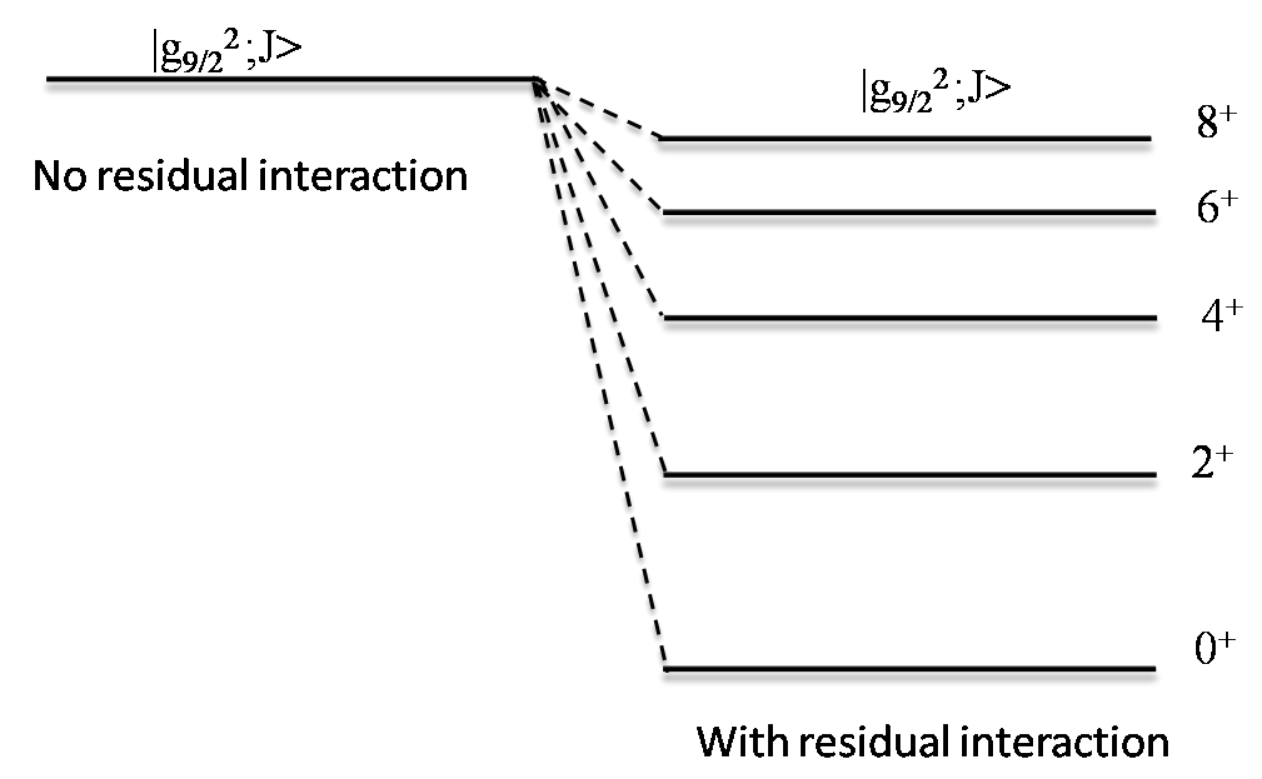
The importance of residual interactions can be easily realized through the energy spectra one obtains for two-particles system. Let us consider two identical nucleons in $g_{9/2}^{2}$ and interacting through a residual interaction $V_{12}$ . The allowed values for the total angular momentum $J$ ranges from $|j_{1}-j_{2}|$ to $j_{1}+j_{2}$ (triangular inequalities), where, $j_{1},j_{2}$ are the angular momentum for the single nucleons. The allowed values for $J$ would be $0,2,4,6,8$ for $g_{9/2}^{2}$ configuration. The resulting $J$ depends on the angle between two orbital planes. A schematic energy level scheme for these two nucleons is shown in Fig. 1, with or without residual interaction. Without residual interaction, all the $J$ states would be degenerate while the states with the inclusion of the residual interaction would be non-degenerate producing significant energy splitting. Residual interaction $V_{12}$ is the strongest when two particles are closest to each other, i.e. when orbitals are co-planar. So, the strongest interaction takes place either for $J_{min}=|j_{1}-j_{2}|=0$ , or $J_{max}=j_{1}+j_{2}=8$ . According to the Pauli principle, no two fermions can occupy the same state/place. Total wave functions must be anti-symmetric.

The wave functions for nucleons are characterized by the spatial co-ordinates and spins. The spatial part of two-nucleon wave function can be decomposed into its center of mass and relative coordinates. The anti-symmetrization of the spatial part of wave-function requires,

	$\displaystyle\Psi(-\vec{r})=-\Psi(\vec{r})$		(3)
	$\displaystyle\text{where}\quad\vec{r}=\vec{r_{2}}-\vec{r_{1}}.$

This ensures that the anti-symmetrized spatial part of wave-function vanishes, if both particles are at the same place, i.e., $\Psi(0)=0$ . On dividing the total wave functions into spatial and spin parts we get,

\displaystyle\Psi_{total}=\Psi_{spatial}(L)\times\Psi_{spin}(S)=Anti-symmetric

(4)

So, there will be two possibilities for $\Psi_{total}$ to be anti-symmetric:
(a) If $\Psi_{spatial}$ is anti-symmetric then $\Psi_{spin}$ would be symmetric.
(b) If $\Psi_{spatial}$ is symmetric then $\Psi_{spin}$ would be anti-symmetric. Also,

	$\displaystyle S=1/2+1/2=1\longrightarrow\Psi_{spin}\quad symmetric,$
	$\displaystyle S=1/2-1/2=0\longrightarrow\Psi_{spin}\quad anti-symmetric.$

Let us consider a simple form of residual interaction, to be a $\delta$ -interaction. The $\delta$ -interaction acts only when $\vec{r}=0$ , requires $\Psi_{spatial}$ to be symmetric. Thus $\delta$ -interaction acts on two identical nucleons with $S=0$ . As a result, the $S=0$ states is lower in energy. For two nucleons in $g_{9/2}^{2}$ , the allowed $J_{min}=0$ would belong to the $S=0$ while $J_{max}=8$ would belong to the $S=1$ . This means that $J=0$ is the lowest since $S=0$ state is lowered due to the action of $\delta$ -interaction as shown schematically in Fig. 1. These general features of the residual interaction can be easily understood in terms of the two-body matrix elements for the $\delta$ -interaction which we cover in the following section.

Refer to caption — Figure 1: A schematic diagram showing the energy levels with and without residual interaction for $g_{9/2}^{2}$ configuration.

3 Matrix elements of $\delta$ -interaction

The simplest interaction potential such as the $\delta$ - and Yukawa forces depends only on the distance between two nucleons. Two-body matrix elements of these interactions are evaluated either by decomposing the two-nucleon wave functions into their center of mass and relative co-ordinates or directly in terms of the two nucleon wave functions which are the anti-symmetrized products or sum of the anti-symmetrized products of a single-nucleon wave function. In the later case, one needs to decompose the interaction potentials into radial and angular parts using the multipole expansion as follows.

3.1 Multipole expansion

The interaction $V(\mathbf{r}_{1},\mathbf{r}_{2})\equiv V(|\mathbf{r}_{1}-\mathbf{r}_{2}|)$ can be expanded in terms of various multipoles as [1, 2],

\displaystyle V(|\mathbf{r}_{1}-\mathbf{r}_{2}|)=\sum_{K=0}^{\infty}V_{K}(r_{1},r_{2})P_{K}(cos\omega_{12}),

(5)

where, $P_{K}(cos\omega_{12})$ is the Legendre polynomial and $\omega_{12}=(\mathbf{r}_{1}\cdot\mathbf{r}_{2})/r_{1}r_{2}$ . The function $V_{K}(r_{1},r_{2})$ are symmetric in $r_{1}$ and $r_{2}$ . Due to the orthogonality relations of Legendre polynomials, the $V_{K}(r_{1},r_{2})$ may be obtained from $V(|\mathbf{r}_{1}-\mathbf{r}_{2}|)$ as,

\displaystyle V_{K}(r_{1},r_{2})=\frac{2K+1}{2}\int_{-1}^{+1}V(|\mathbf{r}_{1}-\mathbf{r}_{2}|)P_{K}(cos\omega_{12})dcos\omega_{12}.

(6)

The Legendre polynomials in the above equation can be expressed by the addition theorem of spherical harmonics as,

\displaystyle P_{K}(cos\omega_{12})=\frac{4\pi}{2K+1}\sum_{q}(-1)^{q}Y^{K}_{q}(\theta_{1},\phi_{1})Y^{K}_{-q}(\theta_{2},\phi_{2}).

(7)

In general, the radial part of the matrix elements is evaluated numerically and it is different for different interactions. However, the angular part of the matrix elements is evaluated analytically and the the procedure to calculate it up to the large extent is similar for most of the interactions.

3.2 $\delta$ -interaction

We now expand the $\delta$ -interaction in terms of the multipoles and evaluate its matrix elements between the anti-symmetrized wave functions for two nucleons. The $\delta$ -interaction between two nucleons is [2],

\delta(\vec{r})=\delta(\vec{r}_{1}-\vec{r}_{2})

(8)

with $\vec{r}=\vec{r}_{1}-\vec{r}_{2}$ , $\vec{r}_{1}$ and $\vec{r}_{2}$ being the coordinates of the two nucleons. The Eq. (8) can be expanded in terms of the multipoles as,

$\displaystyle\delta(\vec{r})$	$\displaystyle=$	$\displaystyle\sum_{K}\frac{\delta(r_{1}-r_{2})}{r_{1}r_{2}}\frac{2K+1}{4\pi}P_{K}(cos\omega_{12})\qquad\text{(multipole decomposition)}$	(9)
	$\displaystyle=$	$\displaystyle\sum_{K}\frac{\delta(r_{1}-r_{2})}{r_{1}r_{2}}\sum_{q}(-1)^{q}Y^{K}_{q}(\theta_{1},\phi_{1})Y^{K}_{-q}(\theta_{2},\phi_{2})$	(10)
	$\displaystyle=$	$\displaystyle\sum_{K}\frac{\delta(r_{1}-r_{2})}{r_{1}r_{2}}Y^{K}(1)\cdot Y^{K}(2),$	(11)

where, $Y^{K}(i)=Y^{K}(\theta_{i},\phi_{i})$ .

The matrix elements of the interaction must be calculated within the anti-symmetrized states for two nucleons whose angular momentums are either coupled or uncoupled. They are usually evaluated within the coupled states of nucleons which are also anti-symmetrized. The anti-symmetrized two-nucleon coupled states can be expressed as,

	$\displaystyle\lvert\alpha_{1}j_{1}\alpha_{2}j_{2};JM\,TM_{T}\rangle_{\bf{as}}$	$\displaystyle=$	$\displaystyle\frac{1}{\sqrt{2(1+\delta_{j_{1}j_{2}}\delta_{t_{1}t_{2}})}}[\lvert\alpha_{1}j_{1}\alpha_{2}j_{2};JM\rangle$
			$\displaystyle-(-1)^{j_{1}+j_{2}+J}(-1)^{t_{1}+t_{2}+T}\lvert\alpha_{2}j_{2}\alpha_{1}j_{1};JM\rangle]$

where, $\alpha_{i}=n_{i},l_{i}$ denotes the principle and orbital quantum numbers, $j_{i}$ and $t_{i}$ are the angular momentum and isospin of $i$ -th nucleon, respectively. The coupled angular momentum (isospin) and its $z$ -components are denoted by $J$ ( $T$ ) and $M$ ( $M_{T}$ ), respectively. Since, the isospin $t_{1}=t_{2}=\frac{1}{2}$ for two nucleons and the interaction considered Eq. (8) is independent of isospin, the matrix element for the interaction would depend on the total isospin $T$ only through the phase factor which ensures the total anti-symmetrization of the two-nucleon wave functions. Hence forth, we retain the isospin quantum number $T$ only in the phase factor. Further, the $\delta$ -interaction conserves the total angular momentum due to its rotational invariance, the matrix elements are non-zero only if the total angular momentum and its $z-$ component in the initial and final states are same. Matrix element of the $\delta$ -interaction between the anti-symmetrized wave function for two nucleons can be written as,

$\displaystyle\langle\alpha_{1}j_{1}\alpha_{2}j_{2};JM\rvert\delta(\vec{r})\lvert\alpha^{\prime}_{1}j^{\prime}_{1}\alpha^{\prime}_{2}j^{\prime}_{2};JM\rangle_{\bf{as}}$	$\displaystyle=$	$\displaystyle N_{12}[\underbrace{\langle\alpha_{1}j_{1}\alpha_{2}j_{2};JM\rvert\delta(\vec{r})\lvert\alpha^{\prime}_{1}j^{\prime}_{1}\alpha^{\prime}_{2}j^{\prime}_{2};JM\rangle}_{direct}$
	$\displaystyle+$	$\displaystyle\underbrace{(-1)^{j^{\prime}_{1}+j^{\prime}_{2}+J+T}\langle\alpha_{1}j_{1}\alpha_{2}j_{2};JM\rvert\delta(\vec{r})\lvert\alpha^{\prime}_{2}j^{\prime}_{2}\alpha^{\prime}_{1}j^{\prime}_{1};JM\rangle}_{exchange}]$
$\displaystyle\text{with}\qquad N_{12}$	$\displaystyle=$	$\displaystyle[(1+\delta_{j_{1}j_{2}})(1+\delta_{j^{\prime}_{1}j^{\prime}_{2}})]^{-1/2}.$	(14)

3.2.1 Direct term

By substituting Eq.(11) in Eq.(3.2), the direct term becomes,

\displaystyle D

\displaystyle=

\displaystyle\langle\alpha_{1}j_{1}\alpha_{2}j_{2};JM\rvert\sum_{K}\frac{\delta(r_{1}-r_{2})}{r_{1}r_{2}}Y^{K}(1)\cdot Y^{K}(2)\lvert\alpha^{\prime}_{1}j^{\prime}_{1}\alpha^{\prime}_{2}j^{\prime}_{2};JM\rangle

(15)

which can be decomposed into the radial and the angular parts. The radial part consists of the matrix element for $\delta(r_{1}-r_{2})/r_{1}r_{2}$ and the angular part corresponds to the matrix element of $Y_{K}(1)\cdot Y_{K}(2)$ . The angular part can be further decomposed into the products of matrix elements for $Y_{K}(1)$ and $Y_{K}(2)$ using Eq. (86). The Eq. (15) simplifies to,

	$\displaystyle D$	$\displaystyle=$	$\displaystyle{4\pi}C_{0}\sum_{K}(-1)^{j_{2}+J+j^{\prime}_{1}}\left\{\begin{matrix}j_{1}&j_{2}&J\\ j^{\prime}_{2}&j^{\prime}_{1}&K\\ \end{matrix}\right\}$		(16)
			$\displaystyle(l_{1}\frac{1}{2};j_{1}\|\|Y^{K}\|\|l^{\prime}_{1}\frac{1}{2};j^{\prime}_{1})(l_{2}\frac{1}{2};j_{2}\|\|Y^{K}\|\|l^{\prime}_{2}\frac{1}{2};j^{\prime}_{2})$		(16)

where $C_{0}$ denotes the radial integral as follows:

	$\displaystyle C_{0}$	$\displaystyle=$	$\displaystyle\frac{1}{4\pi}\int R^{}_{n_{1}l_{1}j_{1}}(r_{1})R^{}_{n_{2}l_{2}j_{2}}(r_{2})\frac{\delta(r_{1}-r_{2})}{r_{1}r_{2}}R_{n^{\prime}_{1}l^{\prime}_{1}j^{\prime}_{1}}(r_{1})R_{n^{\prime}_{2}l^{\prime}_{2}j^{\prime}_{2}}(r_{2})r_{1}^{2}r_{2}^{2}dr_{1}dr_{2}$		(17)
		$\displaystyle=$	$\displaystyle\frac{1}{4\pi}\int R^{}_{n_{1}l_{1}j_{1}}(r)R^{}_{n_{2}l_{2}j_{2}}(r)R_{n^{\prime}_{1}l^{\prime}_{1}j^{\prime}_{1}}(r)R_{n^{\prime}_{2}l^{\prime}_{2}j^{\prime}_{2}}(r)r^{2}dr$		(17)

The reduced matrix elements appearing in Eq. (16) can be simplified using Eq.(1) as,

$\displaystyle(l_{1}\frac{1}{2};j_{1}\|\|Y^{K}\|\|l^{\prime}_{1}\frac{1}{2};j^{\prime}_{1})$	$\displaystyle=$	$\displaystyle(-1)^{j_{1}-\frac{1}{2}}\left(\frac{\hat{j^{\prime}_{1}}\hat{j_{1}}\hat{K}}{\sqrt{4\pi}}\right)$	(18)
		$\displaystyle\frac{1}{2}(1+(-1)^{l^{\prime}_{1}+l_{1}+K})\times\left(\begin{matrix}j_{1}&K&j^{\prime}_{1}\\ -\frac{1}{2}&0&\frac{1}{2}\end{matrix}\right)$	(18)
$\displaystyle(l_{1}\frac{1}{2};j_{1}\|\|Y^{K}\|\|l^{\prime}_{1}\frac{1}{2};j^{\prime}_{1})(l_{2}\frac{1}{2};j_{2}\|\|Y^{K}\|\|l^{\prime}_{2}\frac{1}{2};j^{\prime}_{2})$	$\displaystyle=$	$\displaystyle(-1)^{j_{1}+j_{2}-1}\left(\frac{\hat{j^{\prime}_{1}}\hat{j_{1}}\hat{j^{\prime}_{2}}\hat{j_{2}}\hat{K}^{2}}{4\pi}\right)$	(19)
		$\displaystyle\frac{1}{4}(1+(-1)^{l^{\prime}_{1}+l_{1}+K})(1+(-1)^{l^{\prime}_{2}+l_{2}+K})$
		$\displaystyle\times\left(\begin{matrix}j_{1}&K&j^{\prime}_{1}\\ -\frac{1}{2}&0&\frac{1}{2}\end{matrix}\right)\left(\begin{matrix}j_{2}&K&j^{\prime}_{2}\\ -\frac{1}{2}&0&\frac{1}{2}\end{matrix}\right)$

In the Eq.(19) $\hat{j}_{i}=\sqrt{2j_{i}+1}$ , $\hat{K}=\sqrt{2K+1}$ . For simplicity, let us consider $l_{i}^{\prime},j_{i}^{\prime}=l_{i},j_{i}$ . So Eq. (19) becomes,

$\displaystyle(l_{1}\frac{1}{2};j_{1}\|\|Y^{K}\|\|l_{1}\frac{1}{2};j_{1})(l_{2}\frac{1}{2};j_{2}\|\|Y^{K}\|\|l_{2}\frac{1}{2};j_{2})$	$\displaystyle=$	$\displaystyle(-1)^{j_{1}+j_{2}-1}\left(\frac{\hat{j_{1}}^{2}\hat{j_{2}}^{2}\hat{K}^{2}}{4\pi}\right)$	(20)
		$\displaystyle\times\left(\begin{matrix}j_{1}&K&j_{1}\\ -\frac{1}{2}&0&\frac{1}{2}\end{matrix}\right)\left(\begin{matrix}j_{2}&K&j_{2}\\ -\frac{1}{2}&0&\frac{1}{2}\end{matrix}\right)$
		$\displaystyle\frac{1}{4}(1+(-1)^{2l_{1}+K})(1+(-1)^{2l_{2}+K})$
	$\displaystyle=$	$\displaystyle(-1)^{j_{1}+j_{2}-1}\left(\frac{\hat{j_{1}}^{2}\hat{j_{2}}^{2}\hat{K}^{2}}{4\pi}\right)\frac{1}{2}(1+(-1)^{K})$
		$\displaystyle\times\left(\begin{matrix}j_{1}&K&j_{1}\\ -\frac{1}{2}&0&\frac{1}{2}\end{matrix}\right)\left(\begin{matrix}j_{2}&K&j_{2}\\ -\frac{1}{2}&0&\frac{1}{2}\end{matrix}\right)$

Substituting Eq. (20) in Eq. (16) we get,

$\displaystyle D$	$\displaystyle=$	$\displaystyle 4\pi C_{0}\sum_{K}(-1)^{j_{2}+J+j_{1}}\left\{\begin{matrix}j_{1}&j_{2}&J\\ j_{2}&j_{1}&K\\ \end{matrix}\right\}(-1)^{j_{1}+j_{2}-1}\left(\frac{\hat{j_{1}}^{2}\hat{j_{2}}^{2}\hat{K}^{2}}{4\pi}\right)$	(21)
		$\displaystyle\frac{1}{2}(1+(-1)^{K})\times\left(\begin{matrix}j_{1}&K&j_{1}\\ -\frac{1}{2}&0&\frac{1}{2}\end{matrix}\right)\left(\begin{matrix}j_{2}&K&j_{2}\\ -\frac{1}{2}&0&\frac{1}{2}\end{matrix}\right)$
	$\displaystyle=$	$\displaystyle C_{0}\left(\frac{\hat{j_{1}}^{2}\hat{j_{2}}^{2}}{2}\right)\sum_{K}(-1)^{J-1}\hat{K}^{2}(1+(-1)^{K})\times\left\{\begin{matrix}j_{1}&j_{2}&J\\ j_{2}&j_{1}&K\\ \end{matrix}\right\}\left(\begin{matrix}j_{1}&K&j_{1}\\ -\frac{1}{2}&0&\frac{1}{2}\end{matrix}\right)\left(\begin{matrix}j_{2}&K&j_{2}\\ -\frac{1}{2}&0&\frac{1}{2}\end{matrix}\right)$
	$\displaystyle=$	$\displaystyle C_{0}\left(\frac{\hat{j_{1}}^{2}\hat{j_{2}}^{2}}{2}\right)\sum_{K}\left[(-1)^{J-1}\hat{K}^{2}\times\left\{\begin{matrix}j_{1}&j_{2}&J\\ j_{2}&j_{1}&K\\ \end{matrix}\right\}\left(\begin{matrix}j_{1}&K&j_{1}\\ -\frac{1}{2}&0&\frac{1}{2}\end{matrix}\right)\left(\begin{matrix}j_{2}&K&j_{2}\\ -\frac{1}{2}&0&\frac{1}{2}\end{matrix}\right)\right.$
		$\displaystyle+(-1)^{J+K-1}\hat{K}^{2}\left.\times\left\{\begin{matrix}j_{1}&j_{2}&J\\ j_{2}&j_{1}&K\\ \end{matrix}\right\}\left(\begin{matrix}j_{1}&K&j_{1}\\ -\frac{1}{2}&0&\frac{1}{2}\end{matrix}\right)\left(\begin{matrix}j_{2}&K&j_{2}\\ -\frac{1}{2}&0&\frac{1}{2}\end{matrix}\right)\right]$

The sum over $K$ in Eq.(21) can be performed analytically. It can be reduced to product of two 3j- symbols using a suitable identity as follows,

	$\displaystyle\displaystyle\sum_{M_{3}}\left(\begin{matrix}j_{1}&j_{2}&J_{3}\\ m_{1}&m_{2}&M_{3}\\ \end{matrix}\right)\left(\begin{matrix}j^{\prime}_{1}&j^{\prime}_{2}&J_{3}\\ m^{\prime}_{1}&m^{\prime}_{2}&-M_{3}\\ \end{matrix}\right)$	$\displaystyle=$	$\displaystyle\displaystyle\sum_{J^{\prime}_{3}M^{\prime}_{3}}(-1)^{j_{3}+j^{\prime}_{3}+m_{1}+m^{\prime}_{1}}\hat{J^{\prime}_{3}}^{2}\left\{\begin{matrix}j_{1}&j_{2}&J_{3}\\ j^{\prime}_{1}&j^{\prime}_{2}&J^{\prime}_{3}\\ \end{matrix}\right\}$		(22)
			$\displaystyle\left(\begin{matrix}j^{\prime}_{1}&j_{2}&J^{\prime}_{3}\\ m^{\prime}_{1}&m_{2}&M^{\prime}_{3}\\ \end{matrix}\right)\left(\begin{matrix}j_{1}&j^{\prime}_{2}&J^{\prime}_{3}\\ m_{1}&m^{\prime}_{2}&-M^{\prime}_{3}\\ \end{matrix}\right)$		(22)

Substituting $J_{3}=J$ , $J_{3}^{\prime}=K$ , $j^{\prime}_{1}=j_{2}$ and $j^{\prime}_{2}=j_{1}$ in Eq. (22) we get,

$\displaystyle\displaystyle\sum_{M_{3}}\left(\begin{matrix}j_{1}&j_{2}&J\\ m_{1}&m_{2}&M_{3}\\ \end{matrix}\right)\left(\begin{matrix}j_{2}&j_{1}&J\\ m^{\prime}_{1}&m^{\prime}_{2}&-M_{3}\\ \end{matrix}\right)$	$\displaystyle=$	$\displaystyle\displaystyle\sum_{KM^{\prime}_{3}}(-1)^{J+K+m_{1}+m^{\prime}_{1}}\hat{K}^{2}\left\{\begin{matrix}j_{1}&j_{2}&J\\ j_{2}&j_{1}&K\\ \end{matrix}\right\}$	(23)
		$\displaystyle\left(\begin{matrix}j_{2}&j_{2}&K\\ m^{\prime}_{1}&m_{2}&M^{\prime}_{3}\\ \end{matrix}\right)\left(\begin{matrix}j_{1}&j_{1}&K\\ m_{1}&m^{\prime}_{2}&-M^{\prime}_{3}\\ \end{matrix}\right)$
	$\displaystyle=$	$\displaystyle\displaystyle\sum_{KM^{\prime}_{3}}(-1)^{J+K+m_{1}+m^{\prime}_{1}}\hat{K}^{2}\left\{\begin{matrix}j_{1}&j_{2}&J\\ j_{2}&j_{1}&K\\ \end{matrix}\right\}$
		$\displaystyle(-1)^{j_{2}+j_{2}+K}\left(\begin{matrix}j_{2}&K&j_{2}\\ m^{\prime}_{1}&M^{\prime}_{3}&m_{2}\\ \end{matrix}\right)$
		$\displaystyle(-1)^{j_{1}+j_{1}+K}\left(\begin{matrix}j_{1}&K&j_{1}\\ m_{1}&-M^{\prime}_{3}&m^{\prime}_{2}\\ \end{matrix}\right)$
	$\displaystyle=$	$\displaystyle\displaystyle\sum_{KM^{\prime}_{3}}(-1)^{J+K+m_{1}+m^{\prime}_{1}}\hat{K}^{2}\left\{\begin{matrix}j_{1}&j_{2}&J\\ j_{2}&j_{1}&K\\ \end{matrix}\right\}$
		$\displaystyle\left(\begin{matrix}j_{2}&K&j_{2}\\ m^{\prime}_{1}&M^{\prime}_{3}&m_{2}\\ \end{matrix}\right)\left(\begin{matrix}j_{1}&K&j_{1}\\ m_{1}&-M^{\prime}_{3}&m^{\prime}_{2}\\ \end{matrix}\right)$

Sums over $M_{3}$ and $M^{\prime}_{3}$ are constrained by,

	$\displaystyle m_{1}+m_{2}+M_{3}$	$\displaystyle=$	$\displaystyle m^{\prime}_{1}+m^{\prime}_{2}-M_{3}=0$
	$\displaystyle m^{\prime}_{1}+m_{2}+M^{\prime}_{3}$	$\displaystyle=$	$\displaystyle m_{1}+m^{\prime}_{2}-M^{\prime}_{3}=0$

Substituting $m_{1}=m^{\prime}_{1}=-1/2$ , $m_{2}=m^{\prime}_{2}=+1/2$ in Eq.(23), the allowed values are $M_{3}=M^{\prime}_{3}=0$

	$\displaystyle\left(\begin{matrix}j_{1}&j_{2}&J\\ -\frac{1}{2}&+\frac{1}{2}&0\\ \end{matrix}\right)\left(\begin{matrix}j_{2}&j_{1}&J\\ -\frac{1}{2}&+\frac{1}{2}&0\\ \end{matrix}\right)$	$\displaystyle=$	$\displaystyle\displaystyle\sum_{K}(-1)^{J+K-1}\hat{K}^{2}\left\{\begin{matrix}j_{1}&j_{2}&J\\ j_{2}&j_{1}&K\\ \end{matrix}\right\}$		(24)
			$\displaystyle\left(\begin{matrix}j_{2}&K&j_{2}\\ -\frac{1}{2}&0&+\frac{1}{2}\\ \end{matrix}\right)\left(\begin{matrix}j_{1}&K&j_{1}\\ -\frac{1}{2}&0&+\frac{1}{2}\\ \end{matrix}\right)$		(24)

Substituting $m_{1}=m_{2}=+1/2$ , $m^{\prime}_{1}=m^{\prime}_{2}=-1/2$ and the allowed values of $M_{3}=-1,M^{\prime}_{3}=0$ in Eq.(23) becomes,

$\displaystyle\left(\begin{matrix}j_{1}&j_{2}&J\\ \frac{1}{2}&+\frac{1}{2}&-1\\ \end{matrix}\right)\left(\begin{matrix}j_{2}&j_{1}&J\\ -\frac{1}{2}&-\frac{1}{2}&1\\ \end{matrix}\right)$	$\displaystyle=$	$\displaystyle\displaystyle\sum_{K}(-1)^{J+K}\hat{K}^{2}\left\{\begin{matrix}j_{1}&j_{2}&J\\ j_{2}&j_{1}&K\\ \end{matrix}\right\}$	(25)
		$\displaystyle\left(\begin{matrix}j_{2}&K&j_{2}\\ -\frac{1}{2}&0&+\frac{1}{2}\\ \end{matrix}\right)\left(\begin{matrix}j_{1}&K&j_{1}\\ \frac{1}{2}&0&-\frac{1}{2}\\ \end{matrix}\right)$
	$\displaystyle=$	$\displaystyle\displaystyle\sum_{K}(-1)^{J+K}\hat{K}^{2}\left\{\begin{matrix}j_{1}&j_{2}&J\\ j_{2}&j_{1}&K\\ \end{matrix}\right\}$
		$\displaystyle\left(\begin{matrix}j_{2}&K&j_{2}\\ -\frac{1}{2}&0&+\frac{1}{2}\\ \end{matrix}\right)(-1)^{2j_{1}+K}\left(\begin{matrix}j_{1}&K&j_{1}\\ -\frac{1}{2}&0&\frac{1}{2}\\ \end{matrix}\right)$
	$\displaystyle=$	$\displaystyle\displaystyle\sum_{K}(-1)^{J-1}\hat{K}^{2}\left\{\begin{matrix}j_{1}&j_{2}&J\\ j_{2}&j_{1}&K\\ \end{matrix}\right\}$
		$\displaystyle\left(\begin{matrix}j_{2}&K&j_{2}\\ -\frac{1}{2}&0&+\frac{1}{2}\\ \end{matrix}\right)\left(\begin{matrix}j_{1}&K&j_{1}\\ -\frac{1}{2}&0&\frac{1}{2}\\ \end{matrix}\right)$

Adding Eqs. (24) and (25), the R.H.S. and L.H.S. become,

$\displaystyle RHS$	$\displaystyle=$	$\displaystyle\displaystyle\sum_{K}(-1)^{J-1}(1+(-1)^{K})\hat{K}^{2}\left\{\begin{matrix}j_{1}&j_{2}&J\\ j_{2}&j_{1}&K\\ \end{matrix}\right\}\left(\begin{matrix}j_{2}&K&j_{2}\\ -\frac{1}{2}&0&+\frac{1}{2}\\ \end{matrix}\right)\left(\begin{matrix}j_{1}&K&j_{1}\\ -\frac{1}{2}&0&\frac{1}{2}\\ \end{matrix}\right)$	(26)
$\displaystyle LHS$	$\displaystyle=$	$\displaystyle\left(\begin{matrix}j_{1}&j_{2}&J\\ \frac{1}{2}&+\frac{1}{2}&-1\\ \end{matrix}\right)\left(\begin{matrix}j_{2}&j_{1}&J\\ -\frac{1}{2}&-\frac{1}{2}&1\\ \end{matrix}\right)+\left(\begin{matrix}j_{1}&j_{2}&J\\ -\frac{1}{2}&+\frac{1}{2}&0\\ \end{matrix}\right)\left(\begin{matrix}j_{2}&j_{1}&J\\ -\frac{1}{2}&+\frac{1}{2}&0\\ \end{matrix}\right)$	(27)
		$\displaystyle=\left(\begin{matrix}j_{1}&j_{2}&J\\ \frac{1}{2}&+\frac{1}{2}&-1\\ \end{matrix}\right)^{2}+\left(\begin{matrix}j_{1}&j_{2}&J\\ -\frac{1}{2}&+\frac{1}{2}&0\\ \end{matrix}\right)^{2}$	(27)

Using the recursion relation for 3j- symbol as in Eq. (2), yields,

	$\displaystyle\left(\begin{matrix}j_{1}&j_{2}&J\\ \frac{1}{2}&\frac{1}{2}&-1\\ \end{matrix}\right)^{2}$	$\displaystyle=$	$\displaystyle\frac{[\hat{j_{1}}^{2}+\hat{j_{2}}^{2}(-1)^{j_{1}+j_{2}+J}]^{2}}{4J(J+1)}\left(\begin{matrix}j_{1}&j_{2}&J\\ -\frac{1}{2}&\frac{1}{2}&0\\ \end{matrix}\right)^{2}$
	$\displaystyle LHS$	$\displaystyle=$	$\displaystyle\left[1+\frac{[\hat{j_{1}}^{2}+\hat{j_{2}}^{2}(-1)^{j_{1}+j_{2}+J}]^{2}}{4J(J+1)}\right]\left(\begin{matrix}j_{1}&j_{2}&J\\ -\frac{1}{2}&\frac{1}{2}&0\\ \end{matrix}\right)^{2}$		(28)

Using Eqs. (21), (26) and (28), the direct term simply becomes,

\displaystyle D

\displaystyle=

\displaystyle C_{0}\left(\frac{\hat{j_{1}}^{2}\hat{j_{2}}^{2}}{2}\right)\times\left[1+\frac{[\hat{j_{1}}^{2}+\hat{j_{2}}^{2}(-1)^{j_{1}+j_{2}+J}]^{2}}{4J(J+1)}\right]\left(\begin{matrix}j_{1}&j_{2}&J\\ -\frac{1}{2}&\frac{1}{2}&0\\ \end{matrix}\right)^{2}

(29)

Let us consider a special case, if $j_{1}=j_{2}=j,$ and $J$ is even, then, second term in Eq. (29) vanishes, and the direct term becomes,

D=C_{0}\left(\frac{\hat{j}^{4}}{2}\right)\left(\begin{matrix}j&j&J\\ -\frac{1}{2}&\frac{1}{2}&0\\ \end{matrix}\right)^{2}

(30)

We shall see below, for this special case, odd values of $J$ are not allowed for the identical nucleons. Since, the contribution from the exchange term in this case is equal and opposite to that for the direct term.

3.2.2 Exchange term

By substituting Eq.(11) in Eq.(3.2) and separating radial and angular parts of matrix elements the exchange term becomes,

	$\displaystyle E$	$\displaystyle=$	$\displaystyle(-1)^{j^{\prime}_{1}+j^{\prime}_{2}+J+T}4\pi C_{0}\times$		(31)
			$\displaystyle\sum_{K}\langle\alpha_{1}j_{1}\alpha_{2}j_{2};JM\rvert Y^{K}(1)\cdot Y^{K}(2)\lvert\alpha^{\prime}_{2}j^{\prime}_{2}\alpha^{\prime}_{1}j^{\prime}_{1};JM\rangle$		(31)

It must be noticed that the radial part of the matrix element $C_{0}$ is same as that for the direct term Eq.(17), because, the $\delta$ -interaction acts only when $\mathbf{r}_{1}=\mathbf{r}_{2}$ . The angular part can further be decomposed into the products of matrix elements for $Y^{K}(1)$ and $Y^{K}(2)$ using Eq. (1). The Eq. (31) simplifies to,

$\displaystyle E$	$\displaystyle=$	$\displaystyle(-1)^{j^{\prime}_{1}+j^{\prime}_{2}+J+T}4\pi C_{0}\sum_{K}(-1)^{j_{2}+J+j^{\prime}_{2}}\left\{\begin{matrix}j_{1}&j_{2}&J\\ j^{\prime}_{1}&j^{\prime}_{2}&K\\ \end{matrix}\right\}$
		$\displaystyle\langle\alpha_{1}j_{1}\rvert\|Y^{K}(1)\|\lvert\alpha^{\prime}_{2}j^{\prime}_{2}\rangle\langle\alpha_{2}j_{2}\rvert\|Y^{K}(2)\|\lvert\alpha^{\prime}_{1}j^{\prime}_{1}\rangle$
$\displaystyle\langle\alpha_{1};j_{1}\rvert\mid Y^{K}\mid\lvert\alpha^{\prime}_{2};j^{\prime}_{2}\rangle$		$\displaystyle\langle\alpha_{2};j_{2}\rvert\mid Y^{K}\mid\lvert\alpha^{\prime}_{1};j^{\prime}_{1}\rangle=(-1)^{j_{1}+j_{2}-1}\left(\frac{\hat{j^{\prime}_{1}}\hat{j_{1}}\hat{j^{\prime}_{2}}\hat{j_{2}}\hat{K}^{2}}{4\pi}\right)$
		$\displaystyle\quad\quad\quad\quad\quad\quad\frac{1}{4}(1+(-1)^{l^{\prime}_{2}+l_{1}+K})(1+(-1)^{l^{\prime}_{1}+l_{2}+K})$
		$\displaystyle\quad\quad\quad\quad\quad\quad\times\left(\begin{matrix}j_{1}&K&j^{\prime}_{2}\\ -\frac{1}{2}&0&\frac{1}{2}\end{matrix}\right)\left(\begin{matrix}j_{2}&K&j^{\prime}_{1}\\ -\frac{1}{2}&0&\frac{1}{2}\end{matrix}\right)$

For $\alpha^{\prime}_{1}j^{\prime}_{1}=\alpha_{1}j_{1}$ and $\alpha^{\prime}_{2}j^{\prime}_{2}=\alpha_{2}j_{2}$ ,

$\displaystyle\langle\alpha_{1};j_{1}\rvert\mid Y^{K}\mid\lvert\alpha_{2};j_{2}\rangle\langle\alpha_{2};j_{2}\rvert\mid Y^{K}\mid\lvert\alpha_{1};j_{1}\rangle$	$\displaystyle=(-1)^{j_{1}+j_{2}-1}\left(\frac{\hat{j_{1}}^{2}\hat{j_{2}}^{2}\hat{K}^{2}}{4\pi}\right)$	(32)
	$\displaystyle\frac{1}{2}(1+(-1)^{l_{1}+l_{2}+K})$
	$\displaystyle\times\left(\begin{matrix}j_{1}&K&j_{2}\\ -\frac{1}{2}&0&\frac{1}{2}\end{matrix}\right)\left(\begin{matrix}j_{2}&K&j_{1}\\ -\frac{1}{2}&0&\frac{1}{2}\end{matrix}\right)$

$\displaystyle E$	$\displaystyle=$	$\displaystyle(-1)^{T}4\pi C_{0}\left(\frac{\hat{j_{1}}^{2}\hat{j_{2}}^{2}}{8\pi}\right)\sum_{K}\hat{K}^{2}(1+(-1)^{l_{1}+l_{2}+K})\times\left\{\begin{matrix}j_{1}&j_{2}&J\\ j_{1}&j_{2}&K\\ \end{matrix}\right\}\left(\begin{matrix}j_{1}&K&j_{2}\\ -\frac{1}{2}&0&\frac{1}{2}\end{matrix}\right)\left(\begin{matrix}j_{2}&K&j_{1}\\ -\frac{1}{2}&0&\frac{1}{2}\end{matrix}\right)$	(33)
	$\displaystyle=$	$\displaystyle(-1)^{T}C_{0}\left(\frac{\hat{j_{1}}^{2}\hat{j_{2}}^{2}}{2}\right)\sum_{K}\left[\hat{K}^{2}\times\left\{\begin{matrix}j_{1}&j_{2}&J\\ j_{1}&j_{2}&K\\ \end{matrix}\right\}\left(\begin{matrix}j_{1}&K&j_{2}\\ -\frac{1}{2}&0&\frac{1}{2}\end{matrix}\right)\left(\begin{matrix}j_{2}&K&j_{1}\\ -\frac{1}{2}&0&\frac{1}{2}\end{matrix}\right)\right.$
		$\displaystyle+(-1)^{l_{1}+l_{2}+K}\hat{K}^{2}\left.\times\left\{\begin{matrix}j_{1}&j_{2}&J\\ j_{1}&j_{2}&K\\ \end{matrix}\right\}\left(\begin{matrix}j_{1}&K&j_{2}\\ -\frac{1}{2}&0&\frac{1}{2}\end{matrix}\right)\left(\begin{matrix}j_{2}&K&j_{1}\\ -\frac{1}{2}&0&\frac{1}{2}\end{matrix}\right)\right]$

The sum over $K$ can be performed analytically as in the case of direct term. Substituting $J_{3}=J$ , $J_{3}^{\prime}=K$ , $j^{\prime}_{1}=j_{1}$ and $j^{\prime}_{2}=j_{2}$ in Eq. (22), we get,

$\displaystyle\displaystyle\sum_{M_{3}}\left(\begin{matrix}j_{1}&j_{2}&J\\ m_{1}&m_{2}&M_{3}\\ \end{matrix}\right)\left(\begin{matrix}j_{1}&j_{2}&J\\ m^{\prime}_{1}&m^{\prime}_{2}&-M_{3}\\ \end{matrix}\right)$	$\displaystyle=$	$\displaystyle\displaystyle\sum_{KM^{\prime}_{3}}(-1)^{J+K+m_{1}+m^{\prime}_{1}}\hat{K}^{2}\left\{\begin{matrix}j_{1}&j_{2}&J\\ j_{1}&j_{2}&K\\ \end{matrix}\right\}$	(34)
		$\displaystyle\left(\begin{matrix}j_{1}&j_{2}&K\\ m^{\prime}_{1}&m_{2}&M^{\prime}_{3}\\ \end{matrix}\right)\left(\begin{matrix}j_{1}&j_{2}&K\\ m_{1}&m^{\prime}_{2}&-M^{\prime}_{3}\\ \end{matrix}\right)$
	$\displaystyle=$	$\displaystyle\displaystyle\sum_{KM^{\prime}_{3}}(-1)^{J+K+m_{1}+m^{\prime}_{1}}\hat{K}^{2}\left\{\begin{matrix}j_{1}&j_{2}&J\\ j_{1}&j_{2}&K\\ \end{matrix}\right\}$
		$\displaystyle(-1)^{j_{2}+j_{2}+K}\left(\begin{matrix}j_{1}&K&j_{2}\\ m^{\prime}_{1}&M^{\prime}_{3}&m_{2}\\ \end{matrix}\right)\left(\begin{matrix}j_{2}&K&j_{1}\\ m^{\prime}_{2}&-M^{\prime}_{3}&m_{1}\\ \end{matrix}\right)$
	$\displaystyle=$	$\displaystyle\displaystyle\sum_{KM^{\prime}_{3}}(-1)^{j_{1}+j_{2}+J+m_{1}+m^{\prime}_{1}}\hat{K}^{2}\left\{\begin{matrix}j_{1}&j_{2}&J\\ j_{1}&j_{2}&K\\ \end{matrix}\right\}$
		$\displaystyle\left(\begin{matrix}j_{1}&K&j_{2}\\ m^{\prime}_{1}&M^{\prime}_{3}&m_{2}\\ \end{matrix}\right)\left(\begin{matrix}j_{2}&K&j_{1}\\ m^{\prime}_{2}&-M^{\prime}_{3}&m_{1}\\ \end{matrix}\right)$

Substituting $m_{1}=m^{\prime}_{1}=-1/2$ , $m_{2}=m^{\prime}_{2}=+1/2$ and the allowed values are $M_{3}=M^{\prime}_{3}=0$

	$\displaystyle\left(\begin{matrix}j_{1}&j_{2}&J\\ -\frac{1}{2}&+\frac{1}{2}&0\\ \end{matrix}\right)\left(\begin{matrix}j_{1}&j_{2}&J\\ -\frac{1}{2}&+\frac{1}{2}&0\\ \end{matrix}\right)$	$\displaystyle=$	$\displaystyle\displaystyle\sum_{K}(-1)^{j_{1}+j_{2}+J-1}\hat{K}^{2}\left\{\begin{matrix}j_{1}&j_{2}&J\\ j_{1}&j_{2}&K\\ \end{matrix}\right\}$		(35)
			$\displaystyle\left(\begin{matrix}j_{1}&K&j_{2}\\ -\frac{1}{2}&0&+\frac{1}{2}\\ \end{matrix}\right)\left(\begin{matrix}j_{2}&K&j_{1}\\ +\frac{1}{2}&0&-\frac{1}{2}\\ \end{matrix}\right)$		(35)

\displaystyle\left(\begin{matrix}j_{1}&j_{2}&J\\ -\frac{1}{2}&+\frac{1}{2}&0\\ \end{matrix}\right)^{2}

\displaystyle=

\displaystyle\displaystyle\sum_{K}(-1)^{J+K-1}\hat{K}^{2}\left\{\begin{matrix}j_{1}&j_{2}&J\\ j_{1}&j_{2}&K\\ \end{matrix}\right\}\left(\begin{matrix}j_{1}&K&j_{2}\\ -\frac{1}{2}&0&+\frac{1}{2}\\ \end{matrix}\right)\left(\begin{matrix}j_{2}&K&j_{1}\\ -\frac{1}{2}&0&+\frac{1}{2}\\ \end{matrix}\right)

(36)

Substituting $m_{1}=m_{2}=+1/2$ , $m^{\prime}_{1}=m^{\prime}_{2}=-1/2$ , and the allowed values of $M_{3}=-1,M^{\prime}_{3}=0$ in Eq.(34) becomes,

	$\displaystyle\left(\begin{matrix}j_{1}&j_{2}&J\\ \frac{1}{2}&+\frac{1}{2}&-1\\ \end{matrix}\right)\left(\begin{matrix}j_{1}&j_{2}&J\\ -\frac{1}{2}&-\frac{1}{2}&1\\ \end{matrix}\right)$	$\displaystyle=$	$\displaystyle\displaystyle\sum_{K}(-1)^{j_{1}+j_{2}+J}\hat{K}^{2}\left\{\begin{matrix}j_{1}&j_{2}&J\\ j_{1}&j_{2}&K\\ \end{matrix}\right\}\left(\begin{matrix}j_{1}&K&j_{2}\\ -\frac{1}{2}&0&+\frac{1}{2}\\ \end{matrix}\right)\left(\begin{matrix}j_{2}&K&j_{1}\\ -\frac{1}{2}&0&+\frac{1}{2}\\ \end{matrix}\right)$
	$\displaystyle\left(\begin{matrix}j_{1}&j_{2}&J\\ \frac{1}{2}&+\frac{1}{2}&-1\\ \end{matrix}\right)^{2}$	$\displaystyle=$	$\displaystyle\displaystyle\sum_{K}\hat{K}^{2}\left\{\begin{matrix}j_{1}&j_{2}&J\\ j_{1}&j_{2}&K\\ \end{matrix}\right\}\left(\begin{matrix}j_{1}&K&j_{2}\\ -\frac{1}{2}&0&+\frac{1}{2}\\ \end{matrix}\right)\left(\begin{matrix}j_{2}&K&j_{1}\\ -\frac{1}{2}&0&+\frac{1}{2}\\ \end{matrix}\right)$		(37)

Substituting Eqs. (36) and (37) in Eq. (33)

	$\displaystyle E$	$\displaystyle=$	$\displaystyle(-1)^{T}C_{0}\left(\frac{\hat{j_{1}}^{2}\hat{j_{2}}^{2}}{2}\right)\left[\left(\begin{matrix}j_{1}&j_{2}&J\\ \frac{1}{2}&+\frac{1}{2}&-1\\ \end{matrix}\right)^{2}+(-1)^{l_{1}+l_{2}+J-1}\left(\begin{matrix}j_{1}&j_{2}&J\\ -\frac{1}{2}&+\frac{1}{2}&0\\ \end{matrix}\right)^{2}\right]$		(38)
		$\displaystyle=$	$\displaystyle(-1)^{T}C_{0}\left(\frac{\hat{j_{1}}^{2}\hat{j_{2}}^{2}}{2}\right)\left[\left(\begin{matrix}j_{1}&j_{2}&J\\ \frac{1}{2}&+\frac{1}{2}&-1\\ \end{matrix}\right)^{2}-(-1)^{l_{1}+l_{2}+J}\left(\begin{matrix}j_{1}&j_{2}&J\\ -\frac{1}{2}&+\frac{1}{2}&0\\ \end{matrix}\right)^{2}\right]$		(38)

Using the recursion relation for 3j-symbol, Eq. (2),

\displaystyle E

\displaystyle=

\displaystyle(-1)^{T}C_{0}\left(\frac{\hat{j_{1}}^{2}\hat{j_{2}}^{2}}{2}\right)\left(\begin{matrix}j_{1}&j_{2}&J\\ -\frac{1}{2}&\frac{1}{2}&0\\ \end{matrix}\right)^{2}\left[\frac{[\hat{j_{1}}^{2}+\hat{j_{2}}^{2}(-1)^{j_{1}+j_{2}+J}]^{2}}{4J(J+1)}-(-1)^{l_{1}+l_{2}+J}\right]

3.2.3 Total matrix element

Total matrix element is the sum of the direct and exchange terms with appropriate normalization factor. Using Eqs. (3.2),(29), and (), the total matrix element can be written as,

$\displaystyle\langle\alpha_{1}j_{1}\alpha_{2}j_{2};JM\rvert\delta(\vec{r})\lvert\alpha_{1}j_{1}\alpha_{2}j_{2};JM\rangle_{\bf{as}}$	$\displaystyle=$	$\displaystyle N_{12}[D+E]$
	$\displaystyle=$	$\displaystyle N_{12}C_{0}\left(\frac{\hat{j_{1}}^{2}\hat{j_{2}}^{2}}{2}\right)\left(\begin{matrix}j_{1}&j_{2}&J\\ -\frac{1}{2}&\frac{1}{2}&0\\ \end{matrix}\right)^{2}$
		$\displaystyle\times\left[1-(-1)^{l_{1}+l_{2}+J+T}+(1+(-1)^{T})\frac{[\hat{j_{1}}^{2}+\hat{j_{2}}^{2}(-1)^{j_{1}+j_{2}+J}]^{2}}{4J(J+1)}\right]$

For the special case, ${\alpha_{i}j_{i}=\alpha j}$ and $N_{12}=\frac{1}{2}$ , the Eq.() becomes,

\displaystyle\langle(\alpha j)^{2};JM\rvert\delta(\vec{r})\lvert(\alpha j)^{2};JM\rangle_{as}

\displaystyle=

\displaystyle C_{0}\left(\frac{\hat{j}^{4}}{4}\right)\times\left(\begin{matrix}j&j&J\\ \frac{1}{2}&-\frac{1}{2}&0\\ \end{matrix}\right)^{2}\left[1-(-1)^{J+T}+(1+(-1)^{T})\frac{\hat{j}^{4}(1-(-1)^{J})^{2}}{4J(J+1)}\right].

For the identical nucleons, $T=1$ , the above matrix element is non-zero only for even values of $J$ and is given by,

	$\displaystyle\langle(\alpha j)^{2};JM\rvert\delta(\vec{r})\lvert(\alpha j)^{2};JM\rangle_{as}$	$\displaystyle=$	$\displaystyle C_{0}\left(\frac{\hat{j}^{4}}{2}\right)\times\left(\begin{matrix}j&j&J\\ \frac{1}{2}&-\frac{1}{2}&0\\ \end{matrix}\right)^{2}$
		$\displaystyle=$	$\displaystyle C_{0}\left(\frac{(2j+1)^{2}}{2}\right)\times\left(\begin{matrix}j&j&J\\ \frac{1}{2}&-\frac{1}{2}&0\\ \end{matrix}\right)^{2}$

Substituting the value of 3j-symbol for $J=0$ and $2$ ,

\langle(\alpha j)^{2};JM\rvert\delta(\vec{r})\lvert(\alpha j)^{2};JM\rangle_{as}=\frac{C_{0}}{8\pi}\left\{\begin{array}[]{c}(2j+1)\qquad\qquad\qquad\qquad\text{for J=0}\\ (2j+1)\left(\frac{(2j-1)(2j+3)}{16j(j+1)}\right)\qquad\text{for J=2}\end{array}\right.

The $\lvert(\alpha j)^{2};00\rangle$ is referred as paired state. The matrix element for the $\delta$ -interaction between the paired states is much larger than those between the unpaired sates i.e.,

\displaystyle\langle(\alpha j)^{2};00\rvert\delta(\vec{r})\lvert(\alpha j)^{2};00\rangle

\displaystyle>>

\displaystyle\langle(\alpha j)^{2};2M\rvert\delta(\vec{r})\lvert(\alpha j)^{2};2M\rangle

The pairing Hamiltonian, as formally defined later in Section 5, mimics the $\delta$ -interaction acting on the paired state so,

\langle j^{2};JM\rvert\hat{H}_{pair}\lvert j^{2};JM\rangle\propto(2j+1)\delta_{J0}

(43)

4 Creation and annihilation of angular momentum coupled state

The creation and annihilation operators for coupled angular momentum states can be conveniently expressed in terms of these operators for single nucleon. The algebra involving these operators become simple due to the application of Wick’s theorem as described below very briefly. The creation operator ’ $a^{\dagger}$ ’ and annihilation operator ’ $a$ ’ for single-nucleon can be defined as,

	$\displaystyle a^{\dagger}_{\alpha}\lvert-\rangle=\lvert\alpha\rangle,$		(44)
	$\displaystyle a_{\beta}\lvert\alpha\rangle=\delta_{\alpha\beta}\lvert-\rangle,$		(45)
	$\displaystyle a\lvert-\rangle=0,$		(46)

where $\lvert-\rangle$ is the vacuum state. The anti-commutation relations for the creation and annihilation operators for single nucleon ’ $a^{\dagger}$ ’ and ’ $a$ ’ are given by,

	$\displaystyle\left\{a^{\dagger}_{\alpha},a^{\dagger}_{\beta}\right\}=\left\{a_{\alpha},a_{\beta}\right\}$	$\displaystyle=$	$\displaystyle 0$
	$\displaystyle\left\{a^{\dagger}_{\alpha},a_{\beta}\right\}$	$\displaystyle=$	$\displaystyle\delta_{\alpha\beta}$		(47)

The normal order product is defined as,

$\displaystyle:a_{\beta}a^{\dagger}_{\gamma}:$	$\displaystyle=$	$\displaystyle-a^{\dagger}_{\gamma}a_{\beta}$	(48)
$\displaystyle:a_{\beta}a^{\dagger}_{\gamma}a^{\dagger}_{\delta}:$	$\displaystyle=$	$\displaystyle a^{\dagger}_{\gamma}a^{\dagger}_{\delta}a_{\beta}$	(49)
$\displaystyle:a_{\alpha}a_{\beta}a^{\dagger}_{\gamma}a^{\dagger}_{\delta}:$	$\displaystyle=$	$\displaystyle a^{\dagger}_{\gamma}a^{\dagger}_{\delta}a_{\alpha}a_{\beta}$	(50)
$\displaystyle\langle-\rvert:a_{\alpha}a_{\beta}a^{\dagger}_{\gamma}a^{\dagger}_{\delta}:\lvert-\rangle$	$\displaystyle=$	$\displaystyle\langle-\rvert a^{\dagger}_{\gamma}a^{\dagger}_{\delta}a_{\alpha}a_{\beta}\lvert-\rangle=0$	(51)

The normal ordered product essentially arranges all the creation operators left to the annihilation operators as should be clear from the above equations. The over all sign is negative only if number of permutations required to shift all the creation operators to the left is odd.

The contractions of two operators are given by,

$\displaystyle\overbracket{a_{\beta}a^{\dagger}_{\gamma}}$	$\displaystyle=$	$\displaystyle\langle-\rvert a_{\beta}a^{\dagger}_{\gamma}\lvert-\rangle=\delta_{\beta\gamma}$
$\displaystyle\overbracket{a^{\dagger}_{\gamma}a_{\beta}}$	$\displaystyle=$	$\displaystyle\langle-\rvert a^{\dagger}_{\gamma}a_{\beta}\lvert-\rangle=0$
$\displaystyle\overbracket{a_{\alpha}a_{\beta}}$	$\displaystyle=$	$\displaystyle\overbracket{a^{\dagger}_{\gamma}a^{\dagger}_{\delta}}=0$

A product of set of creation and annihilation operators can be simplified in terms of normal order products and contractions using Wick’s theorem. For example, the product of a set of four creation and annihilation operators can be expressed using the Wick’s theorem as,

\displaystyle a_{\alpha}a_{\beta}a^{\dagger}_{\gamma}a^{\dagger}_{\delta}

\displaystyle=

\displaystyle:a_{\alpha}a_{\beta}a^{\dagger}_{\gamma}a^{\dagger}_{\delta}:+\sum_{singles}\overbracket{aa^{\dagger}}:aa^{\dagger}:+\sum_{doubles}\overbracket{aa^{\dagger}}\overbracket{aa^{\dagger}}

(53)

The sums in the above equation run over all the possible single and double contractions. The Eq.(53) can easily be extended to a product of any number of creation and annihilation operators.

4.1 Coupled states

The coupled state of two nucleons can be expressed in terms of product of the single-nucleon states as [2, 3, 4, 5],

\displaystyle\lvert j_{1}j_{2};JM\rangle

\displaystyle=

\displaystyle\sum_{m_{1},m_{2}}\langle j_{1}m_{1}j_{2}m_{2}|j_{1}j_{2}JM\rangle\lvert j_{1}m_{1}j_{2}m_{2}\rangle

(54)

where, $j_{i}$ and $m_{i}$ are the angular momentum and its $z$ -component for the single-nucleon, respectively. The $\langle j_{1}m_{1}j_{2}m_{2}|j_{1}j_{2}JM\rangle$ is the Clebsch-Gordan coefficient. The anti-symmetrization of the above equation yields,

	$\displaystyle\lvert j_{1}j_{2};JM\rangle_{as}$	$\displaystyle=$	$\displaystyle{\mathcal{N}}\sum_{m_{1},m_{2}}\langle j_{1}m_{1}j_{2}m_{2}\|j_{1}j_{2}JM\rangle(\lvert j_{1}m_{1}j_{2}m_{2}\rangle-\lvert j_{2}m_{2}j_{1}m_{1}\rangle)$		(55)
		$\displaystyle=$	$\displaystyle{\mathcal{N}}\sum_{m_{1},m_{2}}\langle j_{1}m_{1}j_{2}m_{2}\|j_{1}j_{2}JM\rangle\lvert j_{1}m_{1}j_{2}m_{2}\rangle_{as}$		(55)

The operators $A^{\dagger}(j_{1},j_{2};JM)$ and $A(j_{1},j_{2};JM)$ which create and annihilate two nucleons in a coupled state can be expressed analogous to Eq. (55) as,

	$\displaystyle{A^{\dagger}}(j_{1}j_{2};JM)$	$\displaystyle=$	$\displaystyle{\mathcal{N}}\sum_{m_{1},m_{2}}\langle j_{1}m_{1}j_{2}m_{2}\|j_{1}j_{2}JM\rangle a^{\dagger}_{j_{1}m_{1}}a^{\dagger}_{j_{2}m_{2}}$		(56)
	$\displaystyle A(j_{1}j_{2};JM)$	$\displaystyle=$	$\displaystyle{\mathcal{N}}\sum_{m_{1},m_{2}}\langle j_{1}m_{1}j_{2}m_{2}\|j_{1}j_{2}JM\rangle a_{j_{2}m_{2}}a_{j_{1}m_{1}}$		(57)

4.1.1 Normalization constant

The normalization constant can easily be calculated by applying Wick’s theorem such that,

\displaystyle\langle\rvert A(j_{1}j_{2};JM)A^{\dagger}(j_{1}j_{2};JM)\lvert-\rangle=1.

(58)

Using Eqs. (56) and (57),

	$\displaystyle\langle-\rvert A(j_{1}j_{2};JM)A^{\dagger}(j_{1}j_{2};JM)\lvert-\rangle$	$\displaystyle=$	$\displaystyle\mathcal{N}^{2}\sum_{m_{1}m_{2}}\sum_{m_{1}^{\prime}m_{2}^{\prime}}\langle j_{1}m_{1}j_{2}m_{2}\|j_{1}j_{2}JM\rangle$
			$\displaystyle\langle j_{1}m^{\prime}_{1}j_{2}m^{\prime}_{2}\|JM\rangle\langle-\rvert a_{j_{2}m^{\prime}_{2}}a_{j_{1}m^{\prime}_{1}}a^{\dagger}_{j_{1}m_{1}}a^{\dagger}_{j_{2}m_{2}}\lvert-\rangle$

The R.H.S. of the Eq.() can be simplified by applying the Wick’s theorem Eq.(53). Also, the vacuum expectation value for a normal ordered product vanishes. Only the fully contracted terms will contribute, we have

	$\displaystyle\langle-\rvert a_{j_{2}m^{\prime}_{2}}a_{j_{1}m^{\prime}_{1}}a^{\dagger}_{j_{1}m_{1}}a^{\dagger}_{j_{2}m_{2}}\lvert-\rangle$	$\displaystyle=$	$\displaystyle\langle-\rvert\left\{\overbracket{a_{j_{2}m^{\prime}_{2}}a^{\dagger}_{j_{2}m_{2}}}\overbracket{a_{j_{1}m^{\prime}_{1}}a^{\dagger}_{j_{1}m_{1}}}-\overbracket{a_{j_{2}m^{\prime}_{2}}a^{\dagger}_{j_{1}m_{1}}}\overbracket{a_{j_{1}m^{\prime}_{1}}a^{\dagger}_{j_{2}m_{2}}}\right\}\lvert-\rangle$
	$\displaystyle\langle-\rvert a_{j_{2}m^{\prime}_{2}}a_{j_{1}m^{\prime}_{1}}a^{\dagger}_{j_{1}m_{1}}a^{\dagger}_{j_{2}m_{2}}\lvert-\rangle$	$\displaystyle=$	$\displaystyle\delta_{m_{1}m_{1}^{\prime}}\delta_{m_{2}m_{2}^{\prime}}-\delta_{j_{1}j_{2}}\delta_{m_{1}m_{2}^{\prime}}\delta_{m_{2}m^{\prime}_{1}}.$		(60)

Substituting Eq. (60) in Eq. (),

$\displaystyle\langle-\rvert A(j_{1}j_{2};JM)A^{\dagger}(j_{1}j_{2};JM)\lvert-\rangle$	$\displaystyle=$	$\displaystyle\mathcal{N}^{2}\sum_{m_{1}m_{2}}\sum_{m_{1}^{\prime}m_{2}^{\prime}}\langle j_{1}m_{1}j_{2}m_{2}\|j_{1}j_{2}JM\rangle\langle j_{1}m^{\prime}_{1}j_{2}m^{\prime}_{2}\|j_{1}j_{2}JM\rangle$	(61)
		$\displaystyle(\delta_{m_{1}m^{\prime}_{1}}\delta_{m_{2}m^{\prime}_{2}}-\delta_{j_{1}j_{2}}\delta_{m_{1}m^{\prime}_{2}}\delta_{m_{2}m^{\prime}_{1}})$
	$\displaystyle=$	$\displaystyle\mathcal{N}^{2}\sum_{m_{1}m_{2}}\left(\langle j_{1}m_{1}j_{2}m_{2}\|j_{1}j_{2}JM\rangle\langle j_{1}m_{1}j_{2}m_{2}\|j_{1}j_{2}JM\rangle\right.$
		$\displaystyle\left.-\delta_{j_{1}j_{2}}\langle j_{1}m_{1}j_{2}m_{2}\|j_{1}j_{2}JM\rangle\langle j_{1}m_{2}j_{2}m_{1}\|j_{1}j_{2}JM\rangle\right)$
	$\displaystyle=$	$\displaystyle\mathcal{N}^{2}\sum_{m_{1}m_{2}}\left(\langle j_{1}m_{1}j_{2}m_{2}\|j_{1}j_{2}JM\rangle^{2}\right.$
		$\displaystyle\left.-\delta_{j_{1}j_{2}}(-1)^{j_{1}+j_{2}-J}\langle j_{1}m_{1}j_{2}m_{2}\|j_{1}j_{2}JM\rangle\langle j_{2}m_{1}j_{1}m_{2}\|j_{1}j_{2}JM\rangle\right)$
	$\displaystyle=$	$\displaystyle\mathcal{N}^{2}\sum_{m_{1}m_{2}}\left(\langle j_{1}m_{1}j_{2}m_{2}\|j_{1}j_{2}JM\rangle^{2}+\delta_{j_{1}j_{2}}(-1)^{-J}\langle j_{1}m_{1}j_{2}m_{2}\|j_{1}j_{2}JM\rangle^{2}\right)$
$\displaystyle\langle-\rvert A(j_{1}j_{2};JM)A^{\dagger}(j_{1}j_{2};JM)\lvert-\rangle$	$\displaystyle=$	$\displaystyle\mathcal{N}^{2}(1+\delta_{j_{1}j_{2}}(-1)^{-J})\sum_{m_{1}m_{2}}\langle j_{1}m_{1}j_{2}m_{2}\|j_{1}j_{2}JM\rangle^{2}$
$\displaystyle\langle-\rvert A(j_{1}j_{2};JM)A^{\dagger}(j_{1}j_{2};JM)\lvert-\rangle$	$\displaystyle=$	$\displaystyle\mathcal{N}^{2}(1+\delta_{j_{1}j_{2}}(-1)^{-J})$
$\displaystyle\mathcal{N}$	$\displaystyle=$	$\displaystyle\frac{1}{\sqrt{1+\delta_{j_{1}j_{2}}}}$	(62)

In Eq.(61) we have substituted $j_{1}=j_{2}$ in the phase factor due to the presence of $\delta_{j_{1}j_{2}}$ . It may be easily verified from Eq. (55) that if $j_{1}=j_{2}$ , only the even value of $J$ are allowed.

5 Pairing Hamiltonian

Two nucleons are said to be in the paired state when, $j_{1}=j_{2}=j,J=M=0$ . The creation and annihilation operators for the paired state can be obtained using Eqs. (56) and (57) together with (62),i.e.,

$\displaystyle{A^{\dagger}}(jj;00)$	$\displaystyle=$	$\displaystyle\frac{1}{\sqrt{2}}\sum_{m_{1},m_{2}}\langle jm_{1}jm_{2}\|jj00\rangle a^{\dagger}_{jm_{1}}a^{\dagger}_{jm_{2}}$	(63)
	$\displaystyle=$	$\displaystyle\frac{1}{\sqrt{2}}\sum_{m}\frac{(-1)^{j-m}}{\sqrt{2j+1}}a^{\dagger}_{jm}a^{\dagger}_{j,-m}$	(63)
$\displaystyle A(jj:00)$	$\displaystyle=$	$\displaystyle\frac{1}{\sqrt{2}}\sum_{m}\frac{(-1)^{j-m}}{\sqrt{2j+1}}a_{j,-m}a_{jm}$	(64)

In the above Eqs. (63) and (64) the operators $A^{\dagger}(jj;00)$ creates a pair while $A(jj;00)$ annihilates it. To facilitate the discussion of pairing Hamiltonian, the operators $A^{\dagger}$ and $A$ can further be simplified as,

	$\displaystyle{A^{\dagger}}(jj;00)$	$\displaystyle=$	$\displaystyle\sqrt{\frac{1}{\Omega}}\sum_{m>0}(-1)^{j-m}a^{\dagger}_{jm}a^{\dagger}_{j,-m}$		(65)
	$\displaystyle A(jj:00)$	$\displaystyle=$	$\displaystyle\sqrt{\frac{1}{\Omega}}\sum_{m>0}(-1)^{j-m}a_{j,-m}a_{jm}$		(66)

where, $\Omega=\frac{1}{2}(2j+1)$ is the pair degeneracy or the maximum number of pairs in a given $j$ -shell.

The pairing Hamiltonian in a single $j$ -shell can be defined as,

\displaystyle\hat{H}_{pair}

\displaystyle=

\displaystyle-GS_{j}^{+}S_{j}^{-}

(67)

where, $G$ is the pairing strength. The operators $S_{j}^{+}S_{j}^{-}$ are the quasi-spin operators as they obey the commutation rules analogous to those for the angular momentum operators (see Appendix A). These operators can be expressed in terms of the pair creation and annihilation operators as,

	$\displaystyle S^{+}_{j}$	$\displaystyle=$	$\displaystyle\sqrt{\Omega}A^{\dagger}=\sum_{m>0}(-1)^{j-m}{a^{\dagger}}_{jm}{a^{\dagger}}_{j,-m}$		(68)
	$\displaystyle S^{-}_{j}$	$\displaystyle=$	$\displaystyle\sqrt{\Omega}A=\sum_{m>0}(-1)^{j-m}a_{j,-m}a_{jm}$		(69)

Using Eqs. (68) and (69), the pairing Hamiltonian can be written as,

\displaystyle\hat{H}_{pair}

\displaystyle=

\displaystyle-G\displaystyle\sum_{m,m^{\prime}>0}(-1)^{2j-m-m^{\prime}}{a^{\dagger}}_{jm}{a^{\dagger}}_{j,-m}a_{j,-m^{\prime}}a_{jm^{\prime}}

It can be easily verified that the matrix element or the pairing Hamiltonian is non-zero only between the paired states, i.e.,

\displaystyle\langle j^{2};JM\rvert\hat{H}_{pair}\lvert j^{2};JM\rangle=\frac{-G}{2}(2j+1)\delta_{J0}\delta_{M0}.

(70)

5.1 Quasi-spin and seniority

The eigen values of the pairing Hamiltonian can be obtained once the commutation relation between $S^{+}_{j}$ and $S^{-}_{j}$ is known. In what follows, we drop the index $j$ from the operators $S^{+}_{j}$ and $S^{-}_{j}$ . This commutation relation can be easily evaluated by applying Wick’s theorem, as briefly described in Appendix A, one gets,

\displaystyle\left[S^{+},S^{-}\right]_{-}=\hat{N}-\Omega=2S^{0}

(71)

where $S^{0}$ is a operator analogous to z-component of quasi spin in a way that $S^{+},S^{-}$ and $S^{0}$ follow the SU(2) Lie algebra (Appendix A). Also, the particle number operator ( $\hat{N}$ ),

\hat{N}=\displaystyle\sum_{m>0}[a^{\dagger}_{m}a_{m}+a^{\dagger}_{-m}a_{-m}].

(72)

It can be further shown that,

	$\displaystyle[S^{+},S^{0}]_{-}=-S^{+}$		(73)
	$\displaystyle\left[S^{-},S^{0}\right]_{-}=S^{-}$		(74)

The commutations of $S^{+},S^{-}$ and $S^{0}$ suggest that these operators follow the angular momentum algebra and can be called as quasi-spin operators. Therefore,

$\displaystyle S^{+}S^{-}$	$\displaystyle=$	$\displaystyle{\bf{S}}^{2}-(S^{0})^{2}+S^{0}$	(75)
	$\displaystyle=$	$\displaystyle S(S+1)-S^{0}(S^{0}-1)$
	$\displaystyle=$	$\displaystyle S(S+1)-\left(\frac{\hat{N}-\Omega}{2}\right)\left(\frac{\hat{N}-\Omega}{2}-1\right)$
	$\displaystyle=$	$\displaystyle S(S+1)-\left(\frac{\Omega-\hat{N}}{2}\right)\left(\frac{\Omega-\hat{N}}{2}+1\right)$

where $S(S+1)$ is the eigen-value for the operator ${\bf{S}}^{2}$ with $S$ being an integer or half-integer analogous to the case of angular momentum. In principle, the eigen-state of the pairing Hamiltonian can be characterized by the quasi-spin $S$ and its $z$ -component $S^{0}$ . However, it is convenient to express them in terms of the total number of nucleons and the seniority quantum number, i.e., number of the unpaired nucleons.

Let us consider a $n$ -nucleon state $\lvert j^{n},\nu;JM\rangle$ with $\nu$ number of unpaired nucleons or the seniority quantum number. Thus, if we consider a state with all the nucleons unpaired, i.e., $n=\nu$ , $\hat{N}\lvert j^{\nu},\nu;JM\rangle=\nu\lvert j^{\nu},\nu;JM\rangle$ and $S^{-}_{j}\lvert j^{\nu},\nu;JM\rangle=0$ , since, there is no pair to annihilate. By operating L.H.S. and R.H.S. of Eq.(75) on $\lvert j^{\nu},\nu;JM\rangle$ ,

$\displaystyle S(S+1)-\left(\frac{\Omega-\hat{N}}{2}\right)\left(\frac{\Omega-\hat{N}}{2}+1\right)\lvert j^{\nu}\nu JM\rangle$	$\displaystyle=$	$\displaystyle S^{+}S^{-}\lvert j^{\nu}\nu JM\rangle$
$\displaystyle S(S+1)-\frac{\Omega-\nu}{2}\left(\frac{\Omega-\nu}{2}+1\right)$	$\displaystyle=$	$\displaystyle 0$
$\displaystyle S$	$\displaystyle=$	$\displaystyle\frac{\Omega-\nu}{2}$

Substituting Eq. (5.1) in Eq. (75),

	$\displaystyle S^{+}S^{-}$	$\displaystyle=$	$\displaystyle\frac{\Omega-\nu}{2}\left(\frac{\Omega-\nu}{2}+1\right)-\left(\frac{\Omega-\hat{N}}{2}\right)\left(\frac{\Omega-\hat{N}}{2}+1\right)$
	$\displaystyle S^{+}S^{-}$	$\displaystyle=$	$\displaystyle\frac{1}{4}(\hat{N}-\nu)(2\Omega-\hat{N}-\nu+2)$		(77)

5.2 Eigen values of $\hat{H}_{pair}$

The pairing Hamiltonian using Eqs. (67) and (77) becomes,

\displaystyle\hat{H}_{pair}

\displaystyle=

\displaystyle-GS^{+}S^{-}=\frac{-G}{4}(\hat{N}-\nu)(2\Omega-\hat{N}-\nu+2)

$\displaystyle\hat{H}_{pair}\lvert j^{n},\nu;JM\rangle$	$\displaystyle=$	$\displaystyle\frac{-G}{4}(\hat{N}-\nu)(2\Omega-\hat{N}-\nu+2)\lvert j^{n},\nu;JM\rangle$
	$\displaystyle=$	$\displaystyle\frac{-G}{4}({n}-\nu)(2\Omega-{n}-\nu+2)\lvert j^{n},\nu;JM\rangle$
	$\displaystyle=$	$\displaystyle E(n,\nu)\lvert j^{n},\nu;JM\rangle$

The pairing eigen value $E(n,\nu)$ can be obtained as,

E(n,\nu)=\frac{-G}{4}({n}-\nu)(2\Omega-{n}-\nu+2)

For fully paired state, $\nu=0$ , in case of even-even nuclei

E(n,0)=\frac{-G}{4}{n}(2\Omega-{n}+2)

The pairing energy is given as,

E(n,\nu)-E(n,0)=\frac{G}{4}{\nu}(2\Omega-{\nu}+2)

(78)

It may be noted that the pairing energy is independent of the number of nucleons in the $j$ -shell.

5.3 Simple applications of Pairing

5.3.1 Even-Even nuclei

One can understand the energy separation of $0^{+}$ and $2^{+}$ in even-even nuclei in terms of pairing. For instance, in Fig. 2 we display the observed spectra for a few nuclei around mass number $A=90$ with the neutron number $N=50$ . It may be noted that the energy separations between the $0^{+}$ and $2^{+}$ for these nuclei are almost $1.4-1.5$ MeV. This is the energy usually required to break one nucleon pair in this mass region. Ground-state for the even-even nuclei corresponds to fully paired state i.e., $J=0^{+}$ , $\nu=0$ . First excited-state corresponds to breaking of one proton pair yielding $J=2^{+}$ , $\nu=2$ . Therefore, within the pairing model, the energy separation between the ground and the first excited states can be approximated using Eq.(78) as,

	$\displaystyle E(2^{+})-E(0^{+})$	$\displaystyle\approx$	$\displaystyle E(n,2)-E(n,0)$
	$\displaystyle E(n,2)-E(n,0)$	$\displaystyle=$	$\displaystyle G\Omega.$		(79)

For $A=90$ mass region, valence nucleons are in orbit $g_{9/2}$ , i.e., $\Omega=5$ , typical value of $G=\frac{25}{A}$ yields,

E(n,2)-E(n,0)\sim 1.4\text{ MeV}

(80)

5.3.2 Odd-A nuclei

Consider ⁴³Ca with three particles in $j=7/2$ orbital outside the closed shell. How do these three angular momenta $j$ couple to give final total $J$ values? The easiest is to use m-scheme. If we use m-scheme for three particles in $j=7/2$ then the allowed $J$ values are $15/2,11/2,9/2,7/2,5/2,3/2$ . For the case of $J=7/2$ two of the particles must have their angular momenta coupled to $J=0$ , giving a total $J=7/2$ from ${(7/2)}^{3}$ configuration. For the $J=15/2,11/2,9/2,5/2$ and $3/2$ , there are no pairs of particles coupled to $J=0$ . Since a $J=0$ pair is the lowest configuration for two particles in the same orbital, $J=7/2$ must lie the lowest for three particles in the same orbital. From ⁴¹Ca to ⁴⁷Ca, odd-A isotopes, ${7/2}^{-}$ state lies as the ground states. These cases are still simple to understand, since as the number of valence nucleons grows, the number of ways of mixing basis states to generate a given $J$ increases rapidly. So, the large-scale shell model calculations are trending in recent times. However, pairing provides a simple physics understanding of such nuclear features.

Figure 2: Energy spectrum of even-even nuclei from mass-90 region.

6 Summary

We have presented detailed derivation for the matrix elements of the $\delta$ -interaction evaluated between anti-symmetrized coupled states. The multipole expansion method used for this purpose enables one to decompose the matrix elements into their respective radial and angular parts. The angular part of the matrix elements are evaluated analytically and the similar procedure can be followed for different interactions. The standard pairing Hamiltonian is then considered whose matrix elements between the paired states are similar to those for the $\delta$ -interaction. The solution for the pairing Hamiltonian is obtained within the quasi-spin formalism. Finally, simple application of the pairing to explain the energy separation between the lowest $0^{+}$ and $2^{+}$ states in the even-even nuclei and the ground state spin for the odd-A nuclei are discussed. Some important relations involving matrix elements for the spherical harmonics and the commutation relations for the quasi-spin operators are presented in the Appendices in order to make the derivation self-contained. The quasi-spin algebra is performed directly in terms of the creation and annihilation operators for single-nucleon together with the application of the Wick’s theorem. These techniques are quite useful in dealing with the mean-field equations for the more general cases such as the Hartree-Fock, Bardeen–Cooper–Schrieffer and Hartree-Fock Bogoliubov theories.

Appendix A Commutation of $S^{+},S^{-}$ and $S^{0}$ operators

The commutation of $S^{+}$ and $S^{-}$ can be expressed using Eqs. (68) and (69) as,

	$\displaystyle\left[S^{+},S^{-}\right]_{-}$	$\displaystyle=$	$\displaystyle\displaystyle\sum_{m,m^{\prime}>0}(-1)^{2j-m-m^{\prime}}[{a^{\dagger}}_{m}{a^{\dagger}}_{-m},a_{-m^{\prime}}a_{m^{\prime}}]_{-}$		(81)
		$\displaystyle=$	$\displaystyle\displaystyle\sum_{m,m^{\prime}>0}(-1)^{2j-m-m^{\prime}}({a^{\dagger}}_{m}{a^{\dagger}}_{-m}a_{-m^{\prime}}a_{m^{\prime}}-a_{-m^{\prime}}a_{m^{\prime}}{a^{\dagger}}_{m}{a^{\dagger}}_{-m}).$		(81)

By applying Wick’s theorem (Eq. (53)) to the 2nd term in Eq.(81),

$\displaystyle a_{-m^{\prime}}a_{m^{\prime}}a^{\dagger}_{m}a^{\dagger}_{-m}$	$\displaystyle=$	$\displaystyle a^{\dagger}_{m}a^{\dagger}_{-m}a_{-m^{\prime}}a_{m^{\prime}}$	(82)
		$\displaystyle+\delta_{-m^{\prime}m}a^{\dagger}_{-m}a_{m^{\prime}}-\delta_{-m^{\prime},-m}a^{\dagger}_{m}a_{m^{\prime}}-\delta_{m^{\prime}m}a^{\dagger}_{-m}a_{-m^{\prime}}+\delta_{m^{\prime},-m}a^{\dagger}_{m}a_{-m^{\prime}}$
		$\displaystyle-\delta_{-m^{\prime}m}\delta_{m^{\prime},-m}+\delta_{-m^{\prime},-m}\delta_{m^{\prime}m}.$

The terms involving single and double Kronecker-delta are due to the single and double contractions, respectively. Substituting Eq. (82) into Eq. (81) we get,

	$\displaystyle\left[S^{+},S^{-}\right]_{-}$	$\displaystyle=$	$\displaystyle\displaystyle\sum_{m,m^{\prime}>0}(-1)^{2j-m-m^{\prime}}[-\delta_{-m^{\prime}m}a^{\dagger}_{-m}a_{m^{\prime}}+\delta_{-m^{\prime},-m}a^{\dagger}_{m}a_{m^{\prime}}+\delta_{m^{\prime}m}a^{\dagger}_{-m}a_{-m^{\prime}}$		(83)
			$\displaystyle-\delta_{m^{\prime},-m}a^{\dagger}_{m}a_{-m^{\prime}}+\delta_{-m^{\prime}m}\delta_{m^{\prime},-m}-\delta_{-m^{\prime},-m}\delta_{m^{\prime}m}]$		(83)

Since sum runs over $m,m^{\prime}>0$ ,

$\displaystyle\left[S^{+},S^{-}\right]_{-}$	$\displaystyle=$	$\displaystyle\displaystyle\sum_{m,m^{\prime}>0}(-1)^{2j-m-m^{\prime}}[+\delta_{-m^{\prime},-m}a^{\dagger}_{m}a_{m^{\prime}}+\delta_{m^{\prime}m}a^{\dagger}_{-m}a_{-m^{\prime}}-\delta_{-m^{\prime},-m}\delta_{m^{\prime}m}]$
	$\displaystyle=$	$\displaystyle\displaystyle\sum_{m>0}(-1)^{2j-2m}[a^{\dagger}_{m}a_{m}+a^{\dagger}_{-m}a_{-m}-1]$
	$\displaystyle=$	$\displaystyle\displaystyle\sum_{m>0}[a^{\dagger}_{m}a_{m}+a^{\dagger}_{-m}a_{-m}-1]$
$\displaystyle\left[S^{+},S^{-}\right]_{-}$	$\displaystyle=$	$\displaystyle\hat{N}-\Omega$	(84)
$\displaystyle\left[S^{+},S^{-}\right]_{-}$	$\displaystyle=$	$\displaystyle 2S^{0}$	(85)

where $\hat{N}=a^{\dagger}_{m}a_{m}+a^{\dagger}_{-m}a_{-m}.$ Similarly, one can show that,

\displaystyle{[S^{+},S^{0}]_{-}=-S^{+}};[S^{-},S^{0}]_{-}=S^{-}

The commutations of $S^{+},S^{-}$ and $S^{0}$ suggest that these operators follow the angular momentum algebra and can be called as quasi-spin operators.

Appendix B Important identities/relations

One often encounters the matrix elements of the scalar product of two spherical harmonics to be evaluated between the coupled states. Such matrix elements are conveniently expressed in terms of the 6j-symbol and the product of the reduced matrix elements of the each of the spherical harmonics. The 6j-symbol contains the geometrical factor of the angular momentum couplings, whereas, the physics is contained in the reduced matrix elements. Following Eq.(10.27) of Ref. [2],

Matrix element of $Y^{K}\cdot Y^{K}$

$\displaystyle\langle\alpha_{1}j_{1}\alpha_{2}j_{2};JM\rvert$	$\displaystyle Y^{K}(1).Y^{K}(2)$	$\displaystyle\lvert\alpha^{\prime}_{1}j^{\prime}_{1}\alpha^{\prime}_{2}j^{\prime}_{2};JM\rangle=(-1)^{j_{2}+J+j^{\prime}_{1}}\left\{\begin{matrix}j_{1}&j_{2}&J\\ j^{\prime}_{2}&j^{\prime}_{1}&K\end{matrix}\right\}$	(86)
		$\displaystyle(\alpha_{1}j_{1}\|\|Y^{K}(1)\|\|\alpha^{\prime}_{1}j^{\prime}_{1})(\alpha_{2}j_{2}\|\|Y^{K}(2)\|\|\alpha^{\prime}_{2}j^{\prime}_{2})$	(86)
$\displaystyle(\alpha_{1}j_{1}\|\|Y^{K}\|\|\alpha^{\prime}_{1}j^{\prime}_{1})$	$\displaystyle\equiv$	$\displaystyle(\frac{1}{2}l_{1}j_{1}\|\|Y^{K}\|\|\frac{1}{2}l^{\prime}_{1}j^{\prime}_{1})$
$\displaystyle(\frac{1}{2}l_{1}j_{1}\|\|Y^{K}\|\|\frac{1}{2}l^{\prime}_{1}j^{\prime}_{1})$	$\displaystyle=$	$\displaystyle(-1)^{j_{1}-1/2}\frac{\hat{j_{1}}\hat{j^{\prime}_{1}}\hat{K}}{\sqrt{4\pi}}$
		$\displaystyle\times\frac{1}{2}[1+(-1)^{l_{1}+l^{\prime}_{1}+K}]\left(\begin{array}[]{ccc}j_{1}&K&j^{\prime}_{1}\\ -\frac{1}{2}&0&\frac{1}{2}\\ \end{array}\right)$

where, $\hat{x}=\sqrt{2x+1}$ .

Recursion relation for 3j-symbols

\displaystyle\left(\begin{matrix}j_{1}&j_{2}&J\\ \frac{1}{2}&\frac{1}{2}&-1\\ \end{matrix}\right)

\displaystyle=

\displaystyle-\frac{1}{2\sqrt{J(J+1)}}[\hat{j}^{2}_{1}+\hat{j}^{2}_{2}(-1)^{j_{1}+j_{2}+J}]\left(\begin{matrix}j_{1}&j_{2}&J\\ -\frac{1}{2}&\frac{1}{2}&0\\ \end{matrix}\right)

Appendix C Matrix elements of spherical harmonics

We provide some details of the derivation for the matrix elements of the spherical harmonics (see Eq. (1)). By using Wigner-Eckart’s theorem [1, 2, 3, 4, 5],

	$\displaystyle\langle lm\|Y^{LM}\|l^{\prime}m^{\prime}\rangle$	$\displaystyle=$	$\displaystyle\int Y^{lm*}Y^{LM}Y^{l^{\prime}m^{\prime}}d\tau$		(91)
		$\displaystyle=$	$\displaystyle{(-1)}^{l-m}\begin{pmatrix}l&L&l^{\prime}\\ -m&M&m^{\prime}\end{pmatrix}\langle l\|\|Y^{L}\|\|l^{\prime}\rangle$		(91)

Also, the scalar product of spherical harmonics,

\displaystyle Y^{l}.Y^{l^{\prime}}=\sum_{m}{(-1)}^{m}Y^{lm}(\theta,\phi)Y^{l^{\prime},-m^{\prime}}(\theta^{\prime},\phi^{\prime})

(92)

is invariant with respect to the rotation of axes. It follows that the scalar product must be a function of angle $\Theta$ between the directions $(\theta,\phi)$ and $(\theta^{\prime},\phi^{\prime})$ . This angle $\Theta$ is the only quantity independent of the choice of axes. Choosing axes so that the direction $(\theta^{\prime},\phi^{\prime})$ becomes the new $z-$ axis,

	$\displaystyle Y^{lm}(\theta,\phi)\rightarrow Y^{lm}(0,0)=\delta_{m,0}$		(93)
	$\displaystyle Y^{l0}(\theta^{\prime},\phi^{\prime})\rightarrow\hat{l}\sqrt{\frac{1}{4\pi}}P_{l}(cos\theta)=\hat{l}\sqrt{\frac{1}{4\pi}}P_{l}(cos\Theta)$		(94)
	$\displaystyle Y^{l}.Y^{l^{\prime}}=\hat{l}\sqrt{\frac{1}{4\pi}}\hat{l^{\prime}}\sqrt{\frac{1}{4\pi}}P_{l}(cos\Theta)$		(95)

where $\hat{l}=\sqrt{2l+1}$ and $\hat{l^{\prime}}=\sqrt{2l^{\prime}+1}$ . Also, if $Y^{lm}(\theta,\phi)$ and $Y^{l^{\prime}m^{\prime}}(\theta^{\prime},\phi^{\prime})$ are spherical harmonics of the same angles $(\theta,\phi)$ then $\sum_{mm^{\prime}}\langle LM|lml^{\prime}m^{\prime}\rangle\hat{l}\sqrt{\frac{1}{4\pi}}\hat{l^{\prime}}\sqrt{\frac{1}{4\pi}}Y^{lm}(\theta,\phi)Y^{l^{\prime}m^{\prime}}(\theta,\phi)$ is a tensor of rank $L$ . That is,

		$\displaystyle\sum_{mm^{\prime}}\langle LM\|lml^{\prime}m^{\prime}\rangle$	$\displaystyle\hat{l}\sqrt{\frac{1}{4\pi}}\hat{l^{\prime}}\sqrt{\frac{1}{4\pi}}Y^{lm}(\theta,\phi)Y^{l^{\prime}m^{\prime}}(\theta,\phi)=A^{L}\hat{L}\sqrt{\frac{1}{4\pi}}Y^{LM}(\theta,\phi)$		(96)
			$\displaystyle=\langle L0\|l0l^{\prime}0\rangle\hat{L}\sqrt{\frac{1}{4\pi}}Y^{LM}(\theta,\phi)$		(96)

where $\hat{L}=\sqrt{2L+1}$ and the value of $A^{L}$ can be found by putting $\theta=0$ , $\phi=0$ .

	$\displaystyle\sum_{m,m^{\prime}}\langle LM\|lml^{\prime}m^{\prime}\rangle\hat{l}\sqrt{\frac{1}{4\pi}}\hat{l^{\prime}}\sqrt{\frac{1}{4\pi}}Y^{lm}(0,0)Y^{l^{\prime}m^{\prime}}(0,0)=A^{L}\hat{L}\sqrt{\frac{1}{4\pi}}Y^{LM}(0,0)$
	$\displaystyle\sum_{m,m^{\prime}}\langle LM\|lml^{\prime}m^{\prime}\rangle\delta_{m,0}\delta_{m^{\prime},0}=A^{L}\delta_{M,0}$
	$\displaystyle\langle L0\|l0l^{\prime}0\rangle=A^{L}$

where $|l-l^{\prime}|\leq L\leq|l+l^{\prime}|$ , and $M=m+m^{\prime}$ . So,

		$\displaystyle Y^{LM}(\theta,\phi)$	$\displaystyle=\sum_{m,m^{\prime}}\frac{\hat{l}\hat{l^{\prime}}}{\hat{L}}\sqrt{\frac{1}{4\pi}}\langle LM\|lml^{\prime}m^{\prime}\rangle\langle L0\|l0l^{\prime}0\rangle Y^{lm}(\theta,\phi)Y^{l^{\prime}m^{\prime}}(\theta,\phi)$
		$\displaystyle Y^{lm}(\theta,\phi)$	$\displaystyle Y^{l^{\prime}m^{\prime}}(\theta,\phi)=\sum_{M}\langle lml^{\prime}m^{\prime}\|LM\rangle\langle l0l^{\prime}0\|L0\rangle\frac{\hat{l}\hat{l^{\prime}}}{\hat{L}}\sqrt{\frac{1}{4\pi}}Y^{LM}(\theta,\phi)$
		$\displaystyle Y^{LM}(\theta,\phi)$	$\displaystyle Y^{l^{\prime}m^{\prime}}(\theta,\phi)=\sum_{m}\langle LMl^{\prime}m^{\prime}\|lm\rangle\langle L0l^{\prime}0\|l0\rangle\frac{\hat{L}\hat{l^{\prime}}}{\hat{l}}\sqrt{\frac{1}{4\pi}}Y^{lm}(\theta,\phi)$

In terms of 3j-symbols,

	$\displaystyle Y^{LM}(\theta,\phi)Y^{l^{\prime}m^{\prime}}(\theta,\phi)$	$\displaystyle=$	$\displaystyle\sum_{m}{(-1)}^{m}\begin{pmatrix}l^{\prime}&L&l\\ m^{\prime}&M&-m\end{pmatrix}\begin{pmatrix}l^{\prime}&L&l\\ 0&0&0\end{pmatrix}$		(97)
			$\displaystyle\hat{L}\hat{l}\hat{l^{\prime}}\sqrt{\frac{1}{4\pi}}Y^{lm}(\theta,\phi)$		(97)

This implies that

$\displaystyle\int Y^{lm*}Y^{LM}Y^{l^{\prime}m^{\prime}}d\tau$	$\displaystyle=$	$\displaystyle\int Y^{lm*}{(-1)}^{m}\begin{pmatrix}l^{\prime}&L&l\\ m^{\prime}&M&-m\end{pmatrix}$	(99)
		$\displaystyle\begin{pmatrix}l^{\prime}&L&l\\ 0&0&0\end{pmatrix}\hat{L}\hat{l}\hat{l^{\prime}}\sqrt{\frac{1}{4\pi}}Y^{lm}d\tau$
	$\displaystyle=$	$\displaystyle{(-1)}^{m}\begin{pmatrix}l^{\prime}&L&l\\ m^{\prime}&M&-m\end{pmatrix}\begin{pmatrix}l^{\prime}&L&l\\ 0&0&0\end{pmatrix}$
		$\displaystyle\hat{L}\hat{l}\hat{l^{\prime}}\sqrt{\frac{1}{4\pi}}$

The last step is due to orthogonality of spherical harmonics. Therefore,

\displaystyle\langle l||Y^{L}||l^{\prime}\rangle={(-1)}^{l}\hat{L}\hat{l}\hat{l^{\prime}}\sqrt{\frac{1}{4\pi}}\begin{pmatrix}l^{\prime}&L&l\\ 0&0&0\end{pmatrix}

(100)

In $|lj\rangle$ -basis, by using Wigner-Eckart theorem,

$\displaystyle\langle lj\|\|Y^{L}\|\|lj^{\prime}\rangle$	$\displaystyle=$	$\displaystyle\langle\frac{1}{2}lj\|\|Y^{L}\|\|\frac{1}{2}l^{\prime}j^{\prime}\rangle$	(101)
	$\displaystyle=$	$\displaystyle{(-1)}^{\frac{1}{2}+l^{\prime}+j+L}\hat{j}\hat{j^{\prime}}$
		$\displaystyle\begin{Bmatrix}l&j&\frac{1}{2}\\ j^{\prime}&l^{\prime}&L\end{Bmatrix}\langle l\|\|Y^{L}\|\|l^{\prime}\rangle\quad$

where

\displaystyle\langle l||Y^{L}||l^{\prime}\rangle={(-1)}^{l}\hat{L}\hat{l}\hat{l^{\prime}}\sqrt{\frac{1}{4\pi}}\begin{pmatrix}l^{\prime}&L&l\\ 0&0&0\end{pmatrix}

Therefore, we need to calculate the term $\begin{Bmatrix}l&j&\frac{1}{2}\\ j^{\prime}&l^{\prime}&L\end{Bmatrix}\begin{pmatrix}l^{\prime}&L&l\\ 0&0&0\end{pmatrix}$ :

$\displaystyle\begin{Bmatrix}l&j&\frac{1}{2}\\ j^{\prime}&l^{\prime}&L\end{Bmatrix}\begin{pmatrix}l^{\prime}&L&l\\ 0&0&0\end{pmatrix}$	$\displaystyle=$	$\displaystyle\begin{Bmatrix}l^{\prime}&L&l\\ j^{\prime}&\frac{1}{2}&j\end{Bmatrix}\begin{pmatrix}l^{\prime}&L&l\\ 0&0&0\end{pmatrix}$	(102)
	$\displaystyle=$	$\displaystyle\sum_{allm^{\prime}s}{(-1)}^{j+j^{\prime}+\frac{1}{2}+m_{s}+m_{j}+m_{j}^{\prime}}\begin{pmatrix}l^{\prime}&L&l\\ 0&0&0\end{pmatrix}$
		$\displaystyle\begin{pmatrix}l^{\prime}&\frac{1}{2}&j^{\prime}\\ 0&m_{s}&-m_{j}^{\prime}\end{pmatrix}\begin{pmatrix}j&L&j^{\prime}\\ -m_{j}&0&m_{j}^{\prime}\end{pmatrix}$
		$\displaystyle\begin{pmatrix}j&\frac{1}{2}&l\\ m_{j}&-m_{s}&0\end{pmatrix}\begin{pmatrix}l^{\prime}&L&l\\ 0&0&0\end{pmatrix}$

Since, $\sum_{m^{\prime}_{l}m_{L}m_{l}}\begin{pmatrix}l^{\prime}&L&l\\ 0&0&0\end{pmatrix}\begin{pmatrix}l^{\prime}&L&l\\ 0&0&0\end{pmatrix}=1$ , however, $m^{\prime}_{l}=m_{L}=m_{l}=0$ . Therefore,

	$\displaystyle\begin{Bmatrix}l&j&\frac{1}{2}\\ j^{\prime}&l^{\prime}&L\end{Bmatrix}\begin{pmatrix}l^{\prime}&L&l\\ 0&0&0\end{pmatrix}$	$\displaystyle=$	$\displaystyle\sum_{m_{s}m_{j}m_{j}^{\prime}}{(-1)}^{j+j^{\prime}+\frac{1}{2}+m_{s}+m_{j}+m_{j}^{\prime}}\begin{pmatrix}l^{\prime}&\frac{1}{2}&j^{\prime}\\ 0&m_{s}&-m_{j}^{\prime}\end{pmatrix}$		(103)
			$\displaystyle\begin{pmatrix}j&L&j^{\prime}\\ -m_{j}&0&m_{j}^{\prime}\end{pmatrix}\begin{pmatrix}j&\frac{1}{2}&l\\ m_{j}&-m_{s}&0\end{pmatrix}$		(103)

3j-symbol is non-zero only if $m_{j}=m_{j}^{\prime}=m_{s}$

	$\displaystyle\begin{Bmatrix}l&j&\frac{1}{2}\\ j^{\prime}&l^{\prime}&L\end{Bmatrix}\begin{pmatrix}l^{\prime}&L&l\\ 0&0&0\end{pmatrix}$	$\displaystyle=$	$\displaystyle\sum_{m_{s}}{(-1)}^{j+j^{\prime}+\frac{1}{2}+m_{s}+m_{s}+m_{s}}\begin{pmatrix}l^{\prime}&\frac{1}{2}&j^{\prime}\\ 0&m_{s}&-m_{s}^{\prime}\end{pmatrix}$
			$\displaystyle\begin{pmatrix}j&L&j^{\prime}\\ -m_{s}&0&m_{s}^{\prime}\end{pmatrix}\begin{pmatrix}j&\frac{1}{2}&l\\ m_{s}&-m_{s}&0\end{pmatrix}$

		$\displaystyle=$	$\displaystyle{(-1)}^{j+j^{\prime}+\frac{1}{2}+3/2}\begin{pmatrix}l^{\prime}&\frac{1}{2}&j^{\prime}\\ 0&\frac{1}{2}&-\frac{1}{2}\end{pmatrix}\begin{pmatrix}j&L&j^{\prime}\\ -\frac{1}{2}&0&\frac{1}{2}\end{pmatrix}\begin{pmatrix}j&\frac{1}{2}&l\\ \frac{1}{2}&-\frac{1}{2}&0\end{pmatrix}$		(104)
			$\displaystyle+{(-1)}^{j+j^{\prime}+\frac{1}{2}-3/2}\begin{pmatrix}l^{\prime}&\frac{1}{2}&j^{\prime}\\ 0&-\frac{1}{2}&\frac{1}{2}\end{pmatrix}\begin{pmatrix}j&L&j^{\prime}\\ \frac{1}{2}&0&-\frac{1}{2}\end{pmatrix}\begin{pmatrix}j&\frac{1}{2}&l\\ -\frac{1}{2}&\frac{1}{2}&0\end{pmatrix}$		(104)

Since, $\begin{pmatrix}j_{1}&j_{2}&j_{3}\\ m_{1}&m_{2}&m_{3}\end{pmatrix}={(-1)}^{j_{1}+j_{2}+j_{3}}\begin{pmatrix}j_{1}&j_{2}&j_{3}\\ -m_{1}&-m_{2}&-m_{3}\end{pmatrix}$ ,

$\displaystyle\begin{Bmatrix}l&j&\frac{1}{2}\\ j^{\prime}&l^{\prime}&L\end{Bmatrix}\begin{pmatrix}l^{\prime}&L&l\\ 0&0&0\end{pmatrix}$	$\displaystyle=$	$\displaystyle[{(-1)}^{j+j^{\prime}+\frac{1}{2}+3/2}$	(105)
		$\displaystyle+{(-1)}^{j+j^{\prime}+\frac{1}{2}-3/2}{(-1)}^{l^{\prime}+\frac{1}{2}+j^{\prime}+j+L+j^{\prime}+j+\frac{1}{2}+l}]$
		$\displaystyle\begin{pmatrix}l^{\prime}&\frac{1}{2}&j^{\prime}\\ 0&\frac{1}{2}&-\frac{1}{2}\end{pmatrix}\begin{pmatrix}j&L&j^{\prime}\\ -\frac{1}{2}&0&\frac{1}{2}\end{pmatrix}\begin{pmatrix}j&\frac{1}{2}&l\\ \frac{1}{2}&-\frac{1}{2}&0\end{pmatrix}$
	$\displaystyle=$	$\displaystyle[{(-1)}^{j+j^{\prime}}+{(-1)}^{j+j^{\prime}-1}{(-1)}^{l+l^{\prime}+1+2j+2j^{\prime}+L}]$
		$\displaystyle\begin{pmatrix}l^{\prime}&\frac{1}{2}&j^{\prime}\\ 0&\frac{1}{2}&-\frac{1}{2}\end{pmatrix}\begin{pmatrix}j&L&j^{\prime}\\ -\frac{1}{2}&0&\frac{1}{2}\end{pmatrix}\begin{pmatrix}j&\frac{1}{2}&l\\ \frac{1}{2}&-\frac{1}{2}&0\end{pmatrix}$
	$\displaystyle=$	$\displaystyle{(-1)}^{j+j^{\prime}}[1+{(-1)}^{l+l^{\prime}+1+L}]$
		$\displaystyle\begin{pmatrix}l^{\prime}&\frac{1}{2}&j^{\prime}\\ 0&\frac{1}{2}&-\frac{1}{2}\end{pmatrix}\begin{pmatrix}j&L&j^{\prime}\\ -\frac{1}{2}&0&\frac{1}{2}\end{pmatrix}\begin{pmatrix}j&\frac{1}{2}&l\\ \frac{1}{2}&-\frac{1}{2}&0\end{pmatrix}$
	$\displaystyle=$	$\displaystyle{(-1)}^{j+j^{\prime}}[1+{(-1)}^{l+l^{\prime}+1+L}]$
		$\displaystyle\frac{{(-1)}^{j^{\prime}-\frac{1}{2}}}{\hat{l^{\prime}}\sqrt{2}}\begin{pmatrix}j&L&j^{\prime}\\ -\frac{1}{2}&0&\frac{1}{2}\end{pmatrix}\frac{{(-1)}^{j-\frac{1}{2}}}{\hat{l}\sqrt{2}}$

Since,

	$\displaystyle\begin{pmatrix}l^{\prime}&\frac{1}{2}&j^{\prime}\\ 0&\frac{1}{2}&-\frac{1}{2}\end{pmatrix}$	$\displaystyle=$	$\displaystyle\begin{pmatrix}j^{\prime}&\frac{1}{2}&l^{\prime}\\ -\frac{1}{2}&\frac{1}{2}&0\end{pmatrix}$
		$\displaystyle=$	$\displaystyle\frac{{(-1)}^{j^{\prime}-\frac{1}{2}}}{\hat{l^{\prime}}\sqrt{2}}\langle j^{\prime}\quad-\frac{1}{2}\quad\frac{1}{2}\quad\frac{1}{2}\|l^{\prime}\quad 0\rangle$

	$\displaystyle\begin{pmatrix}j^{\prime}&\frac{1}{2}&l^{\prime}\\ -\frac{1}{2}&\frac{1}{2}&0\end{pmatrix}=\frac{{(-1)}^{j^{\prime}-\frac{1}{2}}}{\hat{l^{\prime}}\sqrt{2}}\frac{1}{\sqrt{2}}$		(106)
	$\displaystyle\text{and}\begin{pmatrix}j&\frac{1}{2}&l\\ \frac{1}{2}&-\frac{1}{2}&0\end{pmatrix}=\frac{{(-1)}^{j-\frac{1}{2}}}{\hat{l}\sqrt{2}}\frac{1}{\sqrt{2}}$		(107)

From Eqs.(105), (106) and (107),

$\displaystyle\begin{Bmatrix}l&j&\frac{1}{2}\\ j^{\prime}&l^{\prime}&L\end{Bmatrix}\begin{pmatrix}l^{\prime}&L&l\\ 0&0&0\end{pmatrix}$	$\displaystyle=$	$\displaystyle{(-1)}^{2j+2j^{\prime}-1}[1+{(-1)}^{l+l^{\prime}+L}]\frac{1}{2\hat{l}\hat{l^{\prime}}}$	(108)
		$\displaystyle\begin{pmatrix}j&L&j^{\prime}\\ -\frac{1}{2}&0&\frac{1}{2}\end{pmatrix}$
	$\displaystyle=$	$\displaystyle\frac{-1}{2\hat{l}\hat{l^{\prime}}}[1+{(-1)}^{l+l^{\prime}+L}]\begin{pmatrix}j&L&j^{\prime}\\ -\frac{1}{2}&0&\frac{1}{2}\end{pmatrix}$
	$\displaystyle=$	$\displaystyle\frac{-1}{2\hat{l}\hat{l^{\prime}}}[1+{(-1)}^{l+l^{\prime}+L}]\begin{pmatrix}j^{\prime}&L&j\\ -\frac{1}{2}&0&\frac{1}{2}\end{pmatrix}\quad\quad$

Since, $\begin{pmatrix}j&L&j^{\prime}\\ -\frac{1}{2}&0&\frac{1}{2}\end{pmatrix}={(-1)}^{j+L+j^{\prime}}\begin{pmatrix}j&L&j^{\prime}\\ \frac{1}{2}&0&-\frac{1}{2}\end{pmatrix}={(-1)}^{2j+2L+2j^{\prime}}\begin{pmatrix}j^{\prime}&L&j\\ -\frac{1}{2}&0&\frac{1}{2}\end{pmatrix}$ . Therefore, the reduced matrix element of spherical harmonics in $|lj>$ -basis can be written as

$\displaystyle\langle lj\|\|Y^{L}\|\|l^{\prime}j^{\prime}\rangle$	$\displaystyle=$	$\displaystyle\langle\frac{1}{2}lj\|\|Y^{L}\|\|\frac{1}{2}l^{\prime}j^{\prime}\rangle$	(109)
	$\displaystyle=$	$\displaystyle{(-1)}^{\frac{1}{2}+l+l^{\prime}+j+L}\hat{j}\hat{j^{\prime}}\hat{l}\hat{l^{\prime}}\hat{L}\sqrt{\frac{1}{4\pi}}$
		$\displaystyle\times\frac{-1}{2\hat{l}\hat{l^{\prime}}}[1+{(-1)}^{l+l^{\prime}+L}]\begin{pmatrix}j&L&j^{\prime}\\ -\frac{1}{2}&0&\frac{1}{2}\end{pmatrix}$
	$\displaystyle=$	$\displaystyle\frac{-1}{2}{(-1)}^{\frac{1}{2}+l+l^{\prime}+j+L}[1+{(-1)}^{l+l^{\prime}+L}]$
		$\displaystyle\hat{j}\hat{j^{\prime}}\hat{L}\sqrt{\frac{1}{4\pi}}\begin{pmatrix}j&L&j^{\prime}\\ -\frac{1}{2}&0&\frac{1}{2}\end{pmatrix}$
	$\displaystyle=$	$\displaystyle\frac{-1}{2}{(-1)}^{j+\frac{1}{2}}[1+{(-1)}^{l+l^{\prime}+L}]$
		$\displaystyle\hat{j}\hat{j^{\prime}}\hat{L}\sqrt{\frac{1}{4\pi}}\begin{pmatrix}j&L&j^{\prime}\\ -\frac{1}{2}&0&\frac{1}{2}\end{pmatrix}$
	$\displaystyle=$	$\displaystyle\frac{1}{2}{(-1)}^{j+3/2}[1+{(-1)}^{l+l^{\prime}+L}]$
		$\displaystyle\hat{j}\hat{j^{\prime}}\hat{L}\sqrt{\frac{1}{4\pi}}\begin{pmatrix}j&L&j^{\prime}\\ -\frac{1}{2}&0&\frac{1}{2}\end{pmatrix}$
	$\displaystyle=$	$\displaystyle\frac{1}{2}{(-1)}^{j+2-\frac{1}{2}}[1+{(-1)}^{l+l^{\prime}+L}]$
		$\displaystyle\hat{j}\hat{j^{\prime}}\hat{L}\sqrt{\frac{1}{4\pi}}\begin{pmatrix}j&L&j^{\prime}\\ -\frac{1}{2}&0&\frac{1}{2}\end{pmatrix}$
	$\displaystyle=$	$\displaystyle\frac{1}{2}{(-1)}^{j-\frac{1}{2}}[1+{(-1)}^{l+l^{\prime}+L}]$
		$\displaystyle\hat{j}\hat{j^{\prime}}\hat{L}\sqrt{\frac{1}{4\pi}}\begin{pmatrix}j&L&j^{\prime}\\ -\frac{1}{2}&0&\frac{1}{2}\end{pmatrix}$

If ${(-1)}^{l+l^{\prime}+L}$ is odd then the reduced matrix element results in zero. On the other hand, if ${(-1)}^{l+l^{\prime}+L}$ is even then

\displaystyle\langle lj||Y^{L}||l^{\prime}j^{\prime}\rangle

\displaystyle=

\displaystyle{(-1)}^{j-\frac{1}{2}}\hat{j}\hat{j^{\prime}}\hat{L}\sqrt{\frac{1}{4\pi}}\begin{pmatrix}j&L&j^{\prime}\\ -\frac{1}{2}&0&\frac{1}{2}\end{pmatrix}\quad\quad

(110)

The final result is independent of $l$ and $l^{\prime}$ .

References

[1] Amos deShalit and Igal Talmi, Nuclear Shell Theory ( Dover Publications Inc.) (1963).
[2] Igal Talmi Simple Model of Complex Nuclei (Harwood Academic Publishers, Switzerland) (1993).
[3] M. K. Pal, Theory of Nuclear Structure (Affiliated East West Press Pvt. Ltd. New Delhi-Madras) (1982).
[4] Kris L.G. Heyde The Nuclear Shell Model, (Springer-Verlag Berlin Heidelberg) (1990).
[5] R. F. Casten Nuclear Structure from a Simple Perspective, (Oxford University Press) (2000).