Bounds on the attractor dimension for low$-Rm$ wall-bound MHD turbulence

In this section, we solve the eigenvalue problem for the dissipation operator $\mathcal{D}_{Ha}$ in a closed box with $L$-periodic boundary conditions in the $x$ and $y$ direction and impermeable and electrically insulating walls located at $z=-L$ and $z=L$. For these boundary conditions, the Laplacian operator is invertible so that the eigenvalue problem for the $\mathcal{D}_{Ha}$ operator can be formulated using non-dimensional variables as:

Here lengths are normalised by $L$, velocities by an unspecified typical velocity $U$, the eigenvalues $\lambda$ by $\nu/L^{2}$ and electric currents by $\sigma BU$. The choice of $U$ is not important since the problem is linear. $\mathbf{v}$ also has to satisfy the same kinematic boundary conditions (7) as $\delta\mathbf{u}$. As in (8), an electric current field $\mathbf{J}$ is associated to $\mathbf{v}$ by:

where $\Omega=\nabla\times\mathbf{v}$. $\mathbf{J}$ must be solenoidal and satisfy the same electric boundary conditions (9) as $\delta\mathbf{j}$ at the walls located at $z=-1$ and $z=1$.
Since $\frac{\partial}{\partial x}$, $\frac{\partial}{\partial y}$ and $\frac{\partial}{\partial z}$ commute with $\mathcal{D}_{Ha}$, each component $v_{x}$, $v_{y}$ and $v_{z}$ of the solution $\mathbf{v}=(v_{i})_{i\in\{x,y,z\}}$ of (14) is of the form:

with $\phi_{i}\in]-\pi,\pi]$ and $\mathbf{k}_{\perp}=k_{x}\mathbf{e}_{x}+k_{y}\mathbf{e}_{y}$. The periodic boundary conditions in the $x$ and $y$ directions impose $(k_{x},k_{y})\in 2\pi\mathbb{Z}^{2}$. $Z_{i}(z)=\sum_{j}A_{i}^{(j)}\exp(K^{(j)}z)$ where $K^{(j)}$ are the complex roots of the dispersion equation obtained by inserting (17) into (14):

There are always two real and two imaginary roots for $K$: $1/\delta$, $-1/\delta$, $i\kappa_{z}$ and $-i\kappa_{z}$ with:

Eventually, each function $Z_{i}(z)$ is of the general form:

Since the operator $\mathcal{D}_{Ha}$ has homogeneous boundary conditions, there is a discrete spectrum of possible values of $\delta$ and $\kappa_{z}$, which is determined by the boundary conditions. We shall now express the boundary conditions for the $Z_{i}$ functions derived in the previous section. The impermeability conditions at $z=-1$ and $z=1$ yield readily:

which, by virtue of the continuity equation (15) implies:

Using (16) to calculate $J_{z}(z=-1)$ and $J_{z}(z=1)$, then using the dispersion equation (18), the electric conditions at the walls located at $z=-1$ and $z=1$ are respectively written:

where $\int Z_{i}(z)=\delta a_{i}\exp(z/\delta)-\delta b_{i}\exp(-z/\delta)-ic_{i}/\kappa_{z}\exp(i\kappa_{z}z)+id_{i}/\kappa_{z}\exp(-i\kappa_{z}z)$.

We shall now use the boundary conditions (22), (23), (24),(25),(26) and (27) to find the sequences of values of $\delta$, $\kappa_{z}$, $\lambda$ as well as the properties of the related Eigenmodes. Equations (22),(23),(24) and (25) impose 4 homogeneous conditions on the 4 coefficients $A_{z}^{1}$, $A_{z}^{2}$, $A_{z}^{3}$ and $A_{z}^{4}$ in the expression of $Z_{z}$. This means that the eigenmodes of the dissipation operator can be divided into two categories.

1) For the modes of the first category, conditions (22),(23),(24) and (25) are redundant so that $Z_{z}\neq 0$. In this case, the determinant formed by those 4 conditions must be zero, which yields:

The sequence of values of $\kappa_{z}$ and $\delta$ is determined by writing that $-\kappa_{z}^{2}$ and $\delta^{2}$ must both be roots of the dispersion equation (18) for given values of $Ha,\lambda,k_{x}$ and $k_{y}$. Eliminating $\lambda$ between (20) and (19) yields the searched condition:

The system formed by (28) and (29) admits exactly one solution for $(\kappa_{z},\delta)$ in each interval $[p\pi/2,(p+1)\pi/2]\times]0,\infty[$ with $p\in\mathbb{Z}-\{0\}$. This defines the sequence of possible values of $\kappa_{z}$ and $\delta$ for given $Ha$, $\lambda$, and $k_{\perp}$. The related eigenmodes have a non zero component along $\mathbf{e}_{z}$. By analogy with the eigenvalue problems which arise in the linear stability theory (see for instance drazin95), we shall call them Orr-Sommerfeld modes.

2) For the modes from the second category, conditions (26), (27),(24) and (25) are not redundant so that $Z_{z}=0$. The continuity equation (15) then imposes that $k_{x}Z_{x}=-k_{y}Z_{y}$ so that the eigenmodes of this category are only determined by the 4 coefficients $A_{x}^{1}$, $A_{x}^{2}$, $A_{x}^{3}$, and $A_{x}^{4}$ (or alternately $A_{y}^{1}$, $A_{y}^{2}$, $A_{y}^{3}$, $A_{y}^{4}$). $\delta$ and $\kappa_{z}$ are then determined using the electric conditions at the walls (22) and (23) which together with (26) and (27) impose 4 homogeneous conditions on the 4 coefficients $A_{x}^{1}$, $A_{x}^{2}$, $A_{x}^{3}$ and $A_{x}^{4}$ : the determinant formed by these conditions has to be zero for the eigenmodes not to be trivial:

Here the system formed by (30) and (29) admits exactly one solution for $(\kappa_{z},\delta)$ in each interval $[p\pi/2,(p+1)\pi/2]\times]0,\infty[$ with $p\in\mathbb{Z}$. The related eigenmodes have no velocity component along $\mathbf{e}_{z}$ and those with $\kappa_{z}<\pi/2$ exhibit only a weak dependence on $z$ so that we may identify them as quasi two-dimensional modes. Following our analogy with linear stability problems, we shall name the modes of this second category Squire modes.
These modes can be explicated by finding the three independent coefficients from $A_{x}^{1}$, $A_{x}^{2}$, $A_{x}^{3}$, and $A_{x}^{4}$. This is done by solving the system formed by (22), (23),(24) and (25), which is at most of rank 3. $Z_{y}$ is obtained by $k_{y}Z_{y}=-k_{x}Z_{x}$ and $Z_{z}=0$. The associated eigenspace has therefore a dimension between 1 and 3.

In summary, for a given value of $Ha$, the eigenvalues $\lambda(k_{\perp},\kappa_{z})$ of the operator $\mathcal{D}_{Ha}$ are given by the dispersion equation (29). For a fixed value of $k_{\perp}$, $\kappa_{z}$ takes one value in $]0,\pi/2[$ and 2 values in each interval $]p\pi/2,(p+1)\pi/2[$ with $p\in\mathbb{Z}-\{0\}$. This defines a discrete sequence of values for $\lambda$, which once sorted by increasing module yields the sequence of the least dissipative eigenmodes of the dissipation operator $\mathcal{D}_{Ha}$. At this point, the eigenmodes of the dissipation operator already exhibit a quite remarkable similarity with the known properties of a flow between 2 parallel plates as each of those modes exhibits ”core” velocity fluctuations of wavelength $(k_{x},k_{y},\kappa_{z})$ as well as exponential boundary layers of thickness $\delta$ along the walls at $z=-1$ and $z=1$.

By sorting the values of $\lambda(k_{\perp},\kappa_{z})$, we are now able to find the minimum of $|\langle\mbox{Tr}\mathcal{D}_{Ha}P_{n}\rangle|$ for any given value of $n$. We shall now perform this task numerically since the values of $\kappa_{z}$ cannot be found analytically. An upper bound for the attractor dimension as a function of $Ha$ and $Re$ then follows immediately. The numerical method is the same as the one already used in the case of a box with $2\pi$-periodic boundary conditions in the 3 directions of space pa03: it consists of sweeping the $(k_{\perp},\kappa_{z})$ plane with the iso-dissipation (iso-$\lambda$) curves, starting at $|\lambda|=0$. For each value of $\lambda$, we count the number of $(k_{\perp},\kappa_{z})$ points enclosed in the corresponding iso-$\lambda$ curve and calculate the sum of $\lambda$ over all of those points. Each point corresponds to an eigenvalue and should therefore be weighed by its multiplicity both when counting those points and building this sum. However it is simpler to build the sum by taking all multiplicities equal to one. The obtained sum for a given value of $n$ is a slightly looser lower bound for $|\langle\mbox{Tr}\mathcal{D}_{Ha}P_{n}\rangle|$, but this may only affect the numerical constants appearing in the final results, and not the dependence on $Ha$, $n$ and $Re$.
The difference between the present case with walls at $z=-1$ and $z=1$ and the periodic case is that the sequence of real values of $\kappa_{z}$ replaces that of $k_{z}$ in the periodic case, which has integer values. It is important to notice that the only imprecision brought by the numerical process is that of the truncation on the sequence of numerical values of $\kappa_{z}$ and $\lambda$, as well as that which results from the resolution of the systems of equations $\{(\ref{eq:orrsomm}),(\ref{eq:diss_kd})\}$ and $\{(\ref{eq:squire}),(\ref{eq:diss_kd})\}$ using the Newton method. However, since each solution of the system is bracketed, there is no risk of finding any spurious eigenvalues. In this sense, the method can be considered to give an exact result. It should also be pointed out that contrarily to the periodic case where $k_{z}$ has integer values, finding the sequence of values of $\kappa_{z}$ requires high precision arithmetics since the numbers involved in (28) and (30) are very high, whereas the values of $\kappa_{z}$ are not. Using the LONG DOUBLE type in C language allows us to reach values of $Ha$ up to $5000$ and $10^{5}$ modes. Computing the sequence of minimal modes for higher values of $Ha$ and $n$ would require the use of multi-precision libraries.
For given values of $n$ and $Ha$, the numerical algorithm yields directly the minimum of $|\langle\mathcal{D}_{Ha}P_{n}\rangle|$, as well as $k_{\perp_{m}}$, $\kappa_{z_{m}}$, $\delta_{min}$, $\delta_{max}$, which are respectively the maximum values of $k_{\perp}$, $\kappa_{z}$, $\delta$, and the minimum value of $\delta$ over the set $n$ least dissipative modes. The value of $n$ for which the trace of the total evolution operator is zero (i.e. $\langle\mbox{Tr}((-\mathcal{D}_{Ha}+\mathcal{B}(.,\mathbf{u}))P_{n})\rangle=0)$ is an upper bound for the attractor dimension. Knowing the minimum of $|\langle\mathcal{D}_{Ha}P_{n}\rangle|$ and using (13), the value of $Re$ for which $n$ is an upper bound for $d_{M}$ is given by $Re=\sqrt{2|\langle\mbox{Tr}(\mathcal{D}_{Ha}P_{n})\rangle|/n}$. The results are plotted on figure 2.

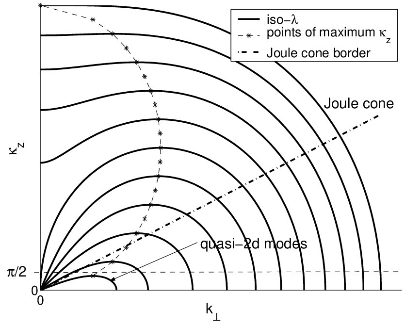
Because the function $\lambda(k_{\perp},\kappa_{z},Ha\sqrt{2})$ has the same expression as the function $1/2\lambda(k_{\perp},k_{z},Ha)$ in the case with periodic boundary conditions in the 3 directions of space pa03, the upper bound for the attractor dimension $d_{M}(Ha,Re)$ in both cases have similar behaviour. As in the periodic case, the maximum values $k_{\perp_{m}}$ and $\kappa_{z_{m}}$ over the set of the $n$ least dissipative modes of $k_{\perp}$ and $\kappa_{z}$ can be deducted from the geometrical shape from the $\lambda(k_{\perp},k_{z})=\lambda_{m}$ curve, where $\lambda_{m}$ is associated to the most dissipative mode of the set (see figure 1).

Increasing progressively the values of $Ha$ for a given value of $Re$, the upper bound for the attractor dimension exhibits three different behaviours which correspond to a 3D isotropic set of modes, a 3D anisotropic set and quasi-2D set respectively. For low values of $Ha$, $d_{M}$ varies little with $Ha$ and the set of eigenmodes of the dissipation which achieve the upper bound is located in a circle centred on the origin in the $(k_{\perp},\kappa_{z})$ plane. If one imagines a flow represented by a combination of such modes, it would be 3D and nearly isotropic. For higher values of $Ha$, $d_{M}\sim Ha^{-1}$, just like in the case with periodic boundary conditions. The least dissipative modes are located within a cardioid-shaped curve, with no modes in the vicinity of the $\kappa_{z}$ axis. A flow featuring such modes would be strongly anisotropic with vortices elongated in the $z$ direction. The boundary between those first two types of sets of modes can be characterised by the disappearance (resp. appearance) of the last (resp. first) mode of the form $(k_{\perp}=0,\kappa_{z}\neq 0)$. When no such modes exist, the tangent at the origin of the iso-$\lambda$ curve corresponding to the most dissipative set of eigenmodes which achieve the upper bound for $d_{M}$ can be defined. All modes are then located under this line which matches the concept of ”Joule Cone” described by sm82: in the existing theories of turbulence, the energy-containing modes are expelled from this cone of axis $(0,k_{z})$ in the Fourier space for high values of $Ha$.
The present case with walls at $z=-1$ and $z=1$ differs from the periodic case for higher values of $Ha$, for which the related set of minimal eigenmodes of the dissipation is quasi two-dimensional. In the periodic case, those modes all satisfy $k_{z}=0$ so that they are strictly two-dimensional and produce no Joule dissipation. In this case, $d_{M}$ doesn’t vary anymore when $Ha$ is increased. In the case with walls, the quasi two dimensional modes are Squire modes with $0<\kappa_{z}<\pi/2$ which exhibit an exponential velocity profile in the vicinity of the wall. This means that the associated values of $|\lambda|$ are higher in the case with walls. When the least dissipative modes are all quasi-2D Squire modes, some dissipation still arises because of the presence of the boundary layer profile at $z=1$ and $z=-1$. This results in $d_{M}$ decreasing rapidly as $Ha$ increases, contrarily to the periodic case. The boundary layer properties of the least dissipative modes are more specifically studied in section IV.4. Also, since the upper bound for the trace of the operator associated to the inertial terms (13) is a general one which relies on no particular assumption on the flow’s three or quasi two-dimensionality, it is unrealistic for two-dimensional flows. An improved upper bound for the attractor dimension in the quasi-2D case is therefore derived in section V, using a quasi two-dimensional model.

For a given value of $Ha$, different types of sets of least dissipative modes are encountered when $n$ (or $Re$) increases. For the sake of clarity, we shall summarise here the 3 boundaries separating those different types of modes and their precise definitions:

• •

  Boundary between quasi-2D and 3D sets of modes:
  Squire modes such that $\kappa_{z}<\pi/2$ are the least dissipative of all and represent quasi-2D velocity fields. A set of modes containing only such modes is quasi-2D. For a given value of $Ha$, the set of the least dissipative modes crosses the quasi-2D- 3D boundary either when the first Orr-Sommerfeld mode or the first squire mode with $\kappa_{z}>\pi/2$ appears.

• •

  ”Joule cone” boundary
  For strong values of $Ha$, the set of least dissipative modes contains no mode located along the $(O,\kappa_{z})$ axis so that all modes are located outside of the Joule cone, defined by the tangent at $(k_{\perp},\kappa_{z})=(0,0)$ to the set of least dissipative modes (see figure 1). No Joule cone can therefore be defined beyond the value of $n$ at which the first mode of the form $(0,0,\kappa_{z})$ appears within the set. This defines what we call the Joule cone boundary, which separates a strongly anisotropic (with Joule cone) from a weakly anisotropic MHD set of modes (without Joule cone).

• •

  Boundary between sets with single and sets with multiple boundary layer thickness
  The evolution of the set of values of $\delta$, reached within the set of the least dissipative modes when $n$ increases, exhibits a sharp transition between sets for which all values are very close to one particular value (for low $n$) and sets with more important scattering (larger $n$). The first one corresponds to a laminar boundary layer state with a well defined thickness, whereas the second exhibits strong similarities with the turbulent Hartmann boundary layer as more quantitatively explained in section IV.4. For a given value of $Ha$, we define this transition as the intersection between the line $\sqrt{2}\delta Ha=1$ and the asymptote to the curve $\delta_{min}(n)$ when $n\rightarrow\infty$ (see figure 3).

When $Ha$ is increased from $0$ for a given value of $n$ or $Re$, these boundaries are encountered in the reverse order. At this point it is important to underline that the properties mentioned in this section are those of the least dissipative modes and not of the real flow. The link between the two is discussed in conclusion.

We shall now derive some analytical estimates for the attractor dimension so as to be able to further compare our results to the results for the size of the dissipative scales available from pa03. We consider separately either side of the Joule cone boundary defined in the previous section, i.e. 3D anisotropic sets of modes (with Joule Cone) and weakly anisotropic 3D sets (without Joule cone).

As the modes are spread uniformly in the Fourier space, with $1/\pi^{3}$ modes per unit of volume, the value of $\lambda_{m}$ can be found by writing that in the $1/8^{th}$ space $k_{x}>0,k_{y}>0,\kappa_{z}>0$, the volume enclosed by the iso-$\lambda_{m}$ curve should be $n/(8\pi^{3})$ . For sufficiently high values of $\kappa_{z_{m}}$ and $k_{\perp_{m}}$, this can be expressed using integrals:

The trace of $\mathcal{D}_{Ha}P_{n}$ similarly expresses as:

The set of $n$ least dissipative modes in the Fourier space is enclosed in the same iso-$\lambda$ curve as the set of $8n/\pi^{3}$ least dissipative modes in the $2\pi-$periodic case. The attractor dimension and the corresponding values of $k_{\perp_{m}}$ are then found by replacing $n$ with $8n/\pi^{3}$ in the results from study with periodic walls (pa03, p3176). Two distinct cases are found:

1) Anisotropic sets of modes (with a Joule cone)
For 3D anisotropic set of least dissipative modes, all modes are located within an elongated cardioid with no mode of the form $k_{\perp}=0$. The Joule cone of axis $(O\kappa_{z})$ exits and its half-angle it that of the tangent at the origin of the iso-$\lambda_{m}$ curve (see figure 1):

All modes are located outside of this cone in the Fourier space. In this case, the upper bound for the attractor dimension is:

and the related bounds for $k_{\perp_{m}}$ and $\kappa_{z_{m}}$ are:

These sets of modes describe are 3D anisotropic. For a 3D anisotropic flow, heuristic considerations of the Kolmogorov type predict $d_{M}\sim Re^{2}/Ha$, $k_{\perp_{m}}\sim Re^{1/2}$ and $k_{z_{m}}\sim Re/Ha$ (see pa03).

2) Weakly anisotropic sets of modes (without Joule cone)
In the case where no Joule cone can be defined within the set of dissipative mode, the related set is quasi-isotropic with:

and corresponding $k_{z_{m}}$ and $\kappa_{z_{m}}$:

In the limits of small Hartmann numbers, (37) recovers the classical hydrodynamic bound for 3D turbulence of $Re^{3}$ (see for instance constantin85_jfm). The boundary between the 3D weakly anisotropic and 3D anisotropic sets of modes can be characterised by the appearance of the Joule cone. This happens when $\sin\theta_{m}=1$, i.e.:

As in the periodic case, the bounds for $d_{M}$, $k_{\perp}$ and $\kappa_{z_{m}}$ exhibit the same dependence on $Ha$ as the heuristic predictions which suggests that our estimate renders the effect of the Lorentz force on the small scales realistically. The powers of $Re$ are however overestimated, but this can be inferred to the estimate for the expansion rate of the inertial terms used in (13) which is known to be too high. The problem of finding an optimal estimate for these terms is to this day still open.
Also, one expects that when the lorentz force becomes of the order of magnitude of inertial effects in the real flow (i.e. $Ha^{2}\gtrsim Re$), the vortices start stretching in the direction of the magnetic field, so fewer of them should be present. Estimates from Kolmogorov-like arguments imply indeed that for a given Reynold number, the number of vortices in the flow without magnetic field ($\sim Re^{3/4}$) is larger than that in a flow with strong magnetic field ($\sim Re/Ha$)as soon as $Ha\gtrsim Re^{-1/4}$. This property is recovered from the results on the upper bound for $d_{M}$ since $d_{M}(Ha)$ clearly decreases when $Ha$ increases at any fixed $Re$ (see figure 2). (34) and (37) however imply that this decrease starts for $Ha>Re$, which in most real cases would correspond to a laminar flow (i.e. $d_{M}=0$ !). This is clearly unrealistic and stems again from the fact that the estimate for the trace of the inertial terms $nRe^{2}$ from which $d_{M}$ is derived for both hydrodynamic and strongly anisotropic MHD flows is even further than the heuristic estimate derived using Kolmorogov-like arguments in the MHD case ($\sim nRe$) than in the hydrodynamic case ($\sim nRe^{3/2}$).

In the two cases of 3D flow with and without Joule cone, the upper bound for the attractor dimension exhibits the same dependence on the non-dimensional numbers as in the case with periodic boundary conditions. This confirms the tendency already observed on the numerical results from the previous section. It also suggests that problems with periodic boundary conditions in the 3 directions of space provide some scaling laws which are relevant to cases involving more realistic boundary conditions like impermeable walls as long as the velocity field is strongly three-dimensional. This relevance however breaks down for quasi two-dimensional velocity fields, the dynamics of which is controlled by the boundary layers which arise along the walls perpendicular to the magnetic field.

We now turn our attention to the influence of the walls on the modes minimising the dissipation, as there lies the most important difference between the periodic case and the case with walls. More precisely, we shall study the values of the boundary layer thickness $\delta$ which characterises the eigenmodes of the dissipation.
As mentioned in section III.1, each mode $(k_{x},k_{y},\kappa_{z})$ can alternately be represented by the triplet $(k_{x},k_{y},\delta)$. Figure 3 represents the evolution of the minimum (resp. maximum) value of $\delta$ reached within the set of the $n$ least dissipative modes $\delta_{min}$ (resp. $\delta_{max}$) as a function of $n$, obtained numerically from $\{(\ref{eq:orrsomm}),(\ref{eq:diss_kd})\}$ and $\{(\ref{eq:squire}),(\ref{eq:diss_kd})\}$. For each fixed value of $Ha$, there is an approximate value $n_{H}$ of $n$, which marks a boundary between two types of sets of least dissipative modes: for $n<n_{H}$, all modes are characterised by a value of $\delta$ close to $1/Ha$ (i.e. $\delta_{min}\simeq\delta{max}$) whereas for $n>n_{H}$, the set of least dissipative modes exhibits a much broader spectrum of values of $\delta$ (i.e. $\delta_{min}<<\delta{max}$). A velocity field represented by a combination of modes taken below this value of $n$ would exhibit a laminar boundary layer of thickness $1/Ha$, with an exponential profile. This matches exactly the prediction of the laminar Hartmann layer theory (see for instance moreau90). For $n>n_{H}$, some modes appear with a thicker boundary layer, as well as modes with a layer much thinner than $1/Ha$. This two-layer structure strongly resembles that of the theoretical prediction of albouss00 for the turbulent Hartmann layer, which also involves such a double deck structure, with a viscous sublayer.

In order to quantify how $n_{H}$ depends on the parameters $Ha$, $n$ and $Re$, we define it quantitatively as the value of $n$ where the line $\delta Ha=1$ (see 3) intersects the asymptote to the curve $\delta_{min}(n)$ for each value of Hartmann and we have plotted the result on figure 4. It is remarkable that the boundary between sets of modes with a single boundary layer thickness and sets with multiple boundary layer thickness is never found between quasi-2D sets of modes, but always where 3D modes are present. This strong property seems to differ from the results of krasnov04 who studied numerically the transition to turbulence of the Hartmann layer in channel flows and found that there can exist a two-dimensional region outside of the turbulent Hartmann layer. A comparison to the real flow in this particular instance is however not straightforward since even if we assume that the flow can indeed be represented by a combination of least dissipative modes some of which are 3D, the flow can still exhibit some 2D features, as explained in conclusion.

These numerical results can be supported by some analytical expressions for the minimum and maximum boundary layer thickness, which can be obtained by eliminating $k_{\perp}^{2}$ between (19) and (20). This defines the iso-$\lambda$ curves in the $(\delta,\kappa_{z})$ plane, which enclose the set of least dissipative modes. Then remarking that the maximum and minimum values of $\delta$ are obtained for $\kappa_{z}=0$ yields the expressions for $\delta_{min}$ and $\delta_{max}$ ²² 2 $\kappa_{z}$ is never zero so these values of $\delta_{min}$ and $\delta_{max}$ are never reached: $\delta_{max}$ is a close upper bound and $\delta_{min}$ is a close lower bound.:

In the case of a 3D set of modes with Joule cone ($1/\sqrt{2}Ha\leq\lambda_{m}\leq Ha^{2}$), $\delta_{min}$ and $\delta_{max}$ are expressed as functions of $Ha$ and $Re$ using (33) and (34):

For low Reynolds numbers (or low values of $|\lambda_{m}|$ in (41) and (42)), $\delta_{min}$ and $\delta_{max}$ are very close to each other, whereas they separate quickly when $\frac{Re}{Ha}$ approaches unity, as confirmed by the numerical results on figure 4. Remarkably, $\frac{Re}{Ha}\sim 1$ coincides also approximately with the disappearance of the Joule cone (40).
As for the turbulent quantities discussed in section IV.1, the boundary layer properties of the least dissipative modes exhibit some striking similarities with that of existing theories moreau90. Quantitatively, the boundary layer thickness associated to those modes has the same dependence on $Ha$ as that of real Hartmann layers. This adds up to the conclusion of pa03 who found that the set of least dissipative modes in a 3D periodic box share many of their properties with those of the real turbulent low (Joule cone angle, small scales, boundary between quasi-2D and 3D sets of modes). Indeed, when walls are present, not only are the turbulent properties of the core flow recovered, but also some of the fine properties of the Hartmann boundary layers are closely mimicked by the least dissipative modes (thickness, boundary between sets of modes with a single boundary layer thickness of $Ha^{-1}$ and sets of modes with multiple thickness.)

References

- (1) Kolmogorov A, N. Local structure of turbulence in an incompressible fluid at very high Reynolds numbers. Dokl. Akad. Nauk. SSSR, 30:299–303, 1941.
- (2) T. Alboussière and R. J. Lingwood. A model for the turbulent Hartmann layer. Phys. Fluids, 12(6):1535–1543, 2000.
- (3) A. Alemany, R. Moreau, P. Sulem, and U. Frish. Influence of an external magnetic field on homogeneous MHD turbulence. Journal de Mécanique, 18(2):277–313, 1979.
- (4) P. Constantin, C. Foias, O.P. Mannley, and R. Temam. Attractors representing turbulent flows. Mem. Am. Math. Soc., 53,314, 1985.
- (5) P. Constantin, C. Foias, O.P. Mannley, and R. Temam. Determining modes and fractal dimension of turbulent flows. J. Fluid. Mech., 150:427–440, 1985.
- (6) P. Constantin, C. Foias, and R. Temam. On the dimension of the attractors in 2D turbulence. physica D, 30:284–296, 1988.
- (7) C.R Doering and J. D. Gibbons. Applied analysis of the Navier-Stokes equation. Cambridge University Press, 1995.
- (8) P. G. Drazin and W.H. Reid. Hydrodynamic stability. Cambridge university press, 1995.
- (9) M. Frank, L. Barleon, and U. Mueller. Visual analysis of two-dimensional magnetohydrodynamics. Phys. Fluids, 13(8):2287–2295, 2001.
- (10) P. Holmes, J.L Lumley, and G. Berkooz. Turbulence, Coherent Structures, Dynamical Systems and Symmetry. Cambridge University Press, 1996.
- (11) H.M. Hua and W.E. Lykoudis. Turbulent measurements in magneto-fluid mechanics channel. Nucl. Sci. Eng., 45:445, 1974.
- (12) V.A. Il’in. Necessary and sufficient condition for the subsystem of eigenfunctions and associated functions of Keldysh’s pencil of ordinary differential operators to form a basis. DAN USSSR, 227(4):796–799 (in Russian), 1976.
- (13) M.V. Keldysh. About eigenvalues and eigenfunctions for some classes of non self-adjoint equations. DAN USSR, 77(14):11–14 (in Russian), 1951.
- (14) M.V. Keldysh. On the completeness of eigenfunctions for certain classes of not self-adjoint linear operators. Russian Mathematics Surveys, 26(4):15–44, 1971.
- (15) R.H. Kraichman. Inertial ranges in two-dimensional turbulence. Phys. Fluids, 10, 1967.
- (16) D. Krasnov, E. Zienicke, O. Zikanov, T. Boeck, and A. Thess. Numerical study of the instability of the Hartmann layer. J. Fluid Mech., 504:183–211, 2004.
- (17) U. Müller L. Bühler. Magnetofluiddynamics in channels and containers. Springer-Verlag, 2001.
- (18) H.K. Moffatt. On the suppression of turbulence by a uniform magnetic field. J. Fluid Mech., 28(3):571–592, 1967.
- (19) R. Moreau. Magnetohydrodynamics. Kluwer Academic Publisher, 1990.
- (20) J. Ohkitani. Log corrected energy spectrum and attractor dimension in two-dimensional turbulence. Phys. Fluids A, 1(3):451–452, 1989.
- (21) A. Pothérat and T. Alboussière. Small scales and anisotropy in low-Rm MHD turbulence. Phys. Fluids, 15 (10):1370–1380, 2003.
- (22) A. Pothérat, J. Sommeria, and R. Moreau. An effective two-dimensional model for MHD flows with transverse magnetic field. J. Fluid Mech., 424:75–100, 2000.
- (23) A. Pothérat, J. Sommeria, and R. Moreau. Numerical simulations of an effective two-dimensional model for flows with a transverse magnetic field. J. Fluid. Mech, 534:115–143, 2005.
- (24) J. Sommeria. Experimental study of the two-dimensionnal inverse energy cascade in a square box. J. Fluid Mech., 170:139–168, 1986.
- (25) Joël Sommeria and René Moreau. Why, how and when MHD turbulence becomes two-dimensional. J. Fluid Mech., 118:507–518, 1982.
- (26) K. Ueno and R. Moreau. Damping rates of magnetohydrodynamic vortices at low magnetic Reynolds number. Phys. Fluids, 18:25105, 2006.
- (27) Wolf. L’histoire de la coulée continue première partie. La revue de la metallurgie, janvier, 1994.