Logical Team Q-learning: An approach towards factored policies in cooperative MARL
Lucas Cassano Ali H. Sayed
École Polytechnique Fédérale de Lausanne École Polytechnique Fédérale de Lausanne
Abstract
We address the challenge of learning factored policies in cooperative MARL scenarios. In particular, we consider the situation in which a team of agents collaborates to optimize a common cost. The goal is to obtain factored policies that determine the individual behavior of each agent so that the resulting joint policy is optimal. The main contribution of this work is the introduction of Logical Team Q-learning (LTQL). LTQL does not rely on assumptions about the environment and hence is generally applicable to any collaborative MARL scenario. We derive LTQL as a stochastic approximation to a dynamic programming method we introduce in this work. We conclude the paper by providing experiments (both in the tabular and deep settings) that illustrate the claims.
1 INTRODUCTION
Reinforcement Learning (RL) has had considerable success in many domains. In particular, Q-learning [Watkins and Dayan, 1992] and its deep learning extension DQN [Mnih et al., 2013] have shown great performance in challenging domains such as the Atari Learning Environment [Bellemare et al., 2013]. At the core of DQN lie two important features: the ability to use expressive function approximators (in particular, neural networks (NN)) that allow it to estimate complex -functions; and the ability to learn off-policy and use replay buffers [Lin, 1992], which allows DQN to be very sample efficient. Traditional RL focuses on the interaction between one agent and an environment. However, in many cases of interest, a multiplicity of agents will need to interact with a unique environment and with each other. This is the object of study of Multi-agent RL (MARL), which goes back to the early work of [Tan, 1993] and has seen renewed interest of late (for an updated survey see [Zhang et al., 2019]). In this paper we consider the particular case of cooperative MARL in which the agents form a team and have a shared unique goal. We are interested in tasks where collaboration is fundamental and a high degree of coordination is necessary to achieve good performance. In particular, we consider two scenarios.
In the first scenario, the global state and all actions are visible to all agents. One example of this situation could be a team of robots that collaborate to move a big and heavy object. It is well known that in this scenario the team can be regarded as one single agent where the aggregate action consists of the joint actions by all agents [Littman, 2001]. The fundamental drawback of this approach is that the joint action space grows exponentially in the number of agents and the problem quickly becomes intractable [Kok and Vlassis, 2004, Guestrin et al., 2002b]. One well-known and popular approach to solve these issues, is to consider each agent as an independent learner (IL) [Tan, 1993]. However, this approach has a number of problems. First, from the point of view of each IL, the environment is non-stationary (due to the changing policies of the other agents), which jeopardizes convergence. And second, replay buffers cannot be used due to the changing nature of the environment and therefore even in cases where this approach might work, the data efficiency of the algorithm is negatively affected. Ideally, it is desirable to derive an algorithm with the following features: i) it learns individual policies (and is therefore scalable), ii) local actions chosen greedily with respect to these individual policies result in an optimal team action, iii) can be combined with NN’s, iv) works off-policy and can leverage replay buffers (for data efficiency), v) and enjoys theoretical guarantees to team optimal policies at least in the dynamic programming scenario. Indeed, the main contribution of this work is the introduction of Logical Team Q-learning (LTQL), an algorithm that has all these properties. We start in the dynamic programing setting and derive equations that characterize the desired solution. We use these equations to define the Factored Team Optimality Bellman Operator and provide a theorem that characterizes the convergence properties of this operator. A stochastic approximation of the dynamic programming setting is used to obtain the tabular and deep versions of our algorithm. For the single agent setting, these steps reduce to: the Bellman optimality equation, the Bellman optimality operator and Q-learning (in its tabular form and DQN).
In the second scenario, we consider the centralized training and decentralized execution paradigm under partial observability. Under this scheme, training is done in a centralized manner and therefore we assume global information to be available during training. During execution, agents only have access to their own observations. Therefore, even though during training global information is available, the learned policies must only rely on local observations. An example of this case would be a soccer team that during training can rely on a centralized server where data is aggregated but has to play games in a fully decentralized manner without the aid of such server.
1.1 Relation to Prior Work
Some of the earliest works on MARL are [Tan, 1993, Claus and Boutilier, 1998]. [Tan, 1993] studied Independent Q-learning (IQL) and identified that IQL learners in a MARL setting may fail to converge due to the non-stationarity of the perceived environment. [Claus and Boutilier, 1998] compared the performance of IQL and joint action learners (JAL) where all agents learn the -values for all the joint actions, and identified the problem of coordination during decentralized execution when multiple optimal policies are available. [Littman, 2001] later provided a proof of convergence for JALs. Recently, [Tampuu et al., 2017] did an experimental study of ILs using DQNS in the Atari game Pong. All these mentioned approaches cannot use experience replay due to the non-stationarity of the preceived environment. Following Hyper Q-learning [Tesauro, 2004], [Foerster et al., 2017] addressed this issue to some extent using fingerprints as proxys to model other agents’ strategies.
[Lauer and Riedmiller, 2000] introduced Distributed Q-learning (DistQ), which in the tabular setting has guaranteed convergence to an optimal policy for deterministic MDPs. However, this algorithm performs very poorly in stochastic scenarios and becomes divergent when combined with function approximation. Later Hysteretic Q-learning (HystQ) was introduced in [Matignon et al., 2007] to improve these two limitations. HystQ is based on a heuristic and can be thought of as a generalization of DistQ. These works also consider the scenario where agents cannot perceive the actions of other agents. They are related to LTQL (from this work) in that they can be considered approximations to our algorithm in the scenario where agents do not have information about other agents’ actions. Recently [Omidshafiei et al., 2017] introduced Dec-HDRQNs for multi-task MARL, which combines HystQ with Recurrent NNs and experience replay (which they recognize is important to achieve high sample efficiency) through the use of Concurrent Experience Replay Trajectories.
[Wang and Sandholm, 2003] introduced OAB, the first algorithm that converges to an optimal Nash equilibrium with probability one in any team Markov game. OAB considers the team scenario where agents observe the full state and joint actions. The main disadvantage of this algorithm is that it requires estimation of the transition kernel and rewards for the joint action state space and also relies on keeping count of state-action visitation, which makes it impractical for MDPs of even moderate size and cannot be combined with function approximators.
[Guestrin et al., 2002a, Guestrin et al., 2002b, Kok and Vlassis, 2004] introduced the idea of factoring the joint -function to handle the scalability issue. These papers have the disadvantage that they require coordination graphs that specify how agents affect each other (the graphs require significant domain knowledge). The main shortcoming of these papers is the factoring model they use, in particular they model the optimal -function (which depends on the joint actions) as a sum of local -functions (where is the number of agents, and each -function considers only the action of its corresponding agent). The main issue with this factorization model is that the optimal -function cannot always be factored in this way, in fact, the tasks for which this model does not hold are typically the ones that require a high degree of coordination, which happen to be the tasks where one is most interested in applying specific MARL approaches as opposed to ILs. The approach we introduce in this paper also considers learning factored -functions. However, the fundamental difference is that the factored relations we estimate always exist and the joint action that results from maximizing these individual -functions is optimal. VDN [Sunehag et al., 2018] and Qmix [Rashid et al., 2018] are two recent deep methods that also factorize the optimal -function assuming additivity and monotonicity, respectively. This factoring is their main limitation since many MARL problems of interest do not satisfy any of these two assumptions. Indeed, [Son et al., 2019] showed that these methods are unable to solve a simple matrix game. Furthermore, the individual policies cannot be used for prediction, since the individual values are not estimates of the return. To improve on the representation limitation due to the factoring assumption, [Son et al., 2019] introduced QTRAN which factors the -function in a more general manner and therefore allows for a wider applicability. The main issue with QTRAN is that although it can approximate a wider class of -functions than VDN and Qmix, the algorithm resorts to other approximations, which degrade its performance in complex environments (see [Rashid et al., 2020]).
Recently, actor-critic strategies have been explored. The algorithm introduced in [Zhang et al., 2018] has the disadvantage that it performs poor credit assignment and as a consequence can easily converge to highly suboptimal strategies (see [Cassano et al., 2019]). [Gupta et al., 2017] introduces policy gradient schemes that also have the credit assignment issue. The algorithm presented by [Foerster et al., 2018] addresses this issue, but does so by learning the team’s joint -function and hence this approach does not address the exponential scalability issue. These methods have the added inconvenience that they are on-policy and hence do not enjoy the data efficiency that off-policy methods can achieve.
2 PROBLEM FORMULATION
We consider a situation where multiple agents form a team and interact with an environment and with each other. We model this interaction as a decentralized partially observable Markov decision process (Dec-POMDP)[Oliehoek et al., 2016], which is defined by the tuple (,,,,,), where, is a set of global states shared by all agents; is the set of of agents; is the observation function for agent , whose output lies in some set of observations ; is the set of actions available to agent ; specifies the probability of transitioning to state from state having taken joint actions ; and is a global reward function. Specifically, is the reward when the team transitions to state from state having taken actions . The reward can be a random variable following some distribution . We clarify that from now on we will refer to the collection of all individual actions as the team’s action, denoted as . Furthermore we will use to refer to the actions of all agents except for action . Therefore we can write . The goal of the team is to maximize the team’s return:
| (1) |
where and are the state and actions at time , respectively, is the team’s policy, is the distribution of initial states, and is the discount factor. We clarify that we use bold font to denote random variables and the notation makes explicit that the expectation is taken with respect to distribution . From now on, we will only make the distributions explicit in cases where doing so makes the equations more clear. Accordingly, the team’s optimal state-action value function () and optimal policy () are given by [Sutton and Barto, 1998]:
| (2a) | ||||
| (2b) | ||||
where . As already mentioned, a team problem of this form can be addressed with any single-agent algorithm. The fundamental inconvenience with this approach is that the joint action space scales exponentially with the number of agents, more specifically (where is the joint action space). Another problem with this approach is that the learned -function cannot be executed in a decentralized manner using the agents’ observations. For these reasons, in the next sections we concern ourselves with learning factored quantities.
3 DYNAMIC PROGRAMMING
Similarly to the way that relation (2b) is used to derive -learning in the single agent setting, the goal of this section is to derive relations in the dynamic programming setting from which we can derive a cooperative MARL algorithm. The following two propositions take the first steps in this direction.
Proposition 1.
For each deterministic team optimal policy, there exist factored functions such that:
| (3a) | ||||
| (3b) | ||||
| (3c) | ||||
| (3d) | ||||
where operator is defined such that if there are multiple arguments that maximize the actions that jointly maximize (3d) are chosen.
Proof.
A simple interpretation of equation (3c) is that is the expected return starting from state when agent takes action while the rest of the team acts in an optimal manner.
Proposition 2.
Each deterministic team optimal policy that can be factored into deterministic policies . Such factored deterministic policies can be obtained as follows:
| (6) |
where is the indicator function.
Propositions 1 and 2 are useful because they show that if the agents learn factored functions that satisfy (3) and act greedily with respect to their corresponding , then the resulting team policy is guaranteed to be optimal and hence they are not subject to the coordination problem identified in [Lauer and Riedmiller, 2000]11 1 This problem arises in situations in which the environment has multiple deterministic team optimal policies and the agents learn factored functions of the form (we remark that these are not the same as ). (we show this in section 5.1). Therefore, an algorithm that learns would satisfy the first two of the five desired properties that were enumerated in the introduction. As a sanity check, note that for the case where there is only one agent, equation (3c) simplifies to the Bellman optimality equation. Although in the single agent case the Bellman optimality operator can be used to obtain (by repeated application of the operator), we cannot do the same with . The fundamental reason for this is stated in proposition 3.
Proposition 3.
Proof.
See Appendix 6.1.
Note that proposition 3 implies that relation (3c) is not sufficient to derive a learning algorithm capable of obtaining a team optimal policy because it can converge to sub-optimal team strategies instead. To avoid this inconvenience, it is necessary to find another relation that is only satisfied by . We can obtain one such relation combining (3a) and (3c):
| (7) |
The sub-optimal Nash fixed points mentioned in proposition 3 do not satisfy relation (7) since by definition the right hand side is equal to . Intuitively, equation (7) is not satisfied by these suboptimal strategies because the considers all possible team actions (while Nash equilibria only consider unilateral deviations).
Definition 1.
LTQL is based on operator , the reason we use relations (3c) and (7) to define this operator instead of just (7), is that using only relation (7) we would derive DistQ that has the shortcomings we discussed in section 1.1. A simple interpretation of operator is the following. Consider a basketball game, in which player has the ball and passes the ball to teammate . If gets distracted, misses the ball and the opposing team ends up scoring, should learn from this experience and modify its policy to not pass the ball? The answer is no, since the poor outcome was player ’s fault. In plain English, from the point of view of some player , what the operator means is “I will only learn from experiences in which my teammates acted according to what I think is the optimal team strategy”. It is easy to see why this kind of stubborn rationale cannot escape Nash equilibria (i.e., agents do not learn when the team deviates from its current best strategy, which obviously is a necessary condition to learn better strategies). The interpretation of the full operator is “I will learn from experiences in which: a) my teammates acted according to what I think is the optimal team strategy; or b) my teammates deviated from what I believe is the optimal strategy and the outcome of such deviation was better than I expected if they had acted according to what I thought was optimal”, which arguably is what a logical player would do (this is the origin of the algorithm’s name). We now proceed to describe the convergence properties of operator .
Lemma 1.
For any , after applications of operator to any set of functions it holds:
| (10) | ||||
| (11) | ||||
| (12) | ||||
| (13) |
where . For the special case where we can lower bound equation (10) as follows:
| (14) |
Proof.
See Appendix 6.2.
Lemma 2.
After applications of operator to any set of functions it holds:
| (15) | ||||
| (16) | ||||
| (17) | ||||
| (18) |
for any . If , probability (15) can be bounded by:
| (19) |
where .
Proof.
See Appendix 6.3.
Lemma 1 indicates that if the initial functions have values that are larger than , after sufficient applications of operator all overestimations will be reduced such that with high probability. Lemma 2 show that if the operator is applied sufficient times to functions that do not overestimate , then the obtained function lie in a small neighborhood of the desired solution with high probability. These results give rise to the following important theorem.
Theorem 1.
Repeated application of the operator to any initial set of -functions followed by an application of operator converge to the -neighborhood () of some set with high probability. For the particular case, where and it holds:
| (20) |
for any , where is a constant that depends on , , , , and the initial functions .
Proof.
Combining the results from lemmas 1 and 2 and setting we get that after applications of operator to any set of functions it holds:
| (21) |
where . Now we proceed to analyze . If and satisfies:
| (22) |
we get:
| (23) |
Using the fact that it follows:
| (24) | ||||
| (25) | ||||
| (26) |
where in we used condition (22) and in we used equation (3a). Combining equations (3) through (26) we get:
| (27) |
Combining equation (27) with the fact that we get:
| (28) |
Relation (28) shows why we include an application of at the end in equation (20). The reason is that if we do not, the -value for suboptimal actions oscillates between and , we illustrate this effect in appendix 6.5. We reiterate that and are only equal when optimal actions are chosen (equation (3a)). is the expected return if agent chooses action and the rest of the team follows an optimal policy, while is the best return that can be achieved if agent chooses action .
4 REINFORCEMENT LEARNING
In this section we present LTQL (see algorithm 1), which we obtain as a stochastic approximation to the procedure described in theorem 1. Note that the algorithm utilizes two estimates for each agent , a biased one parameterized by (which we denote ) and an unbiased one parameterized by (which we denote ). We clarify that in the listing of LTQL is the accumulate and add operator and that we used a constant step-size, however this can be replaced with decaying step-sizes or other schemes such as AdaGrad [Duchi et al., 2011] or Adam [Kingma and Ba, 2014]. Note that the target of the unbiased network is used to calculate the target values for both functions; this prevents the bias in the estimates (which arises due to the condition)22 2 We refer to the condition of the first if statement (i.e., ) as , and the condition corresponding to the second if statement as . from propagating through bootstrapping. The target parameters of the biased estimates () are used solely to evaluate condition . We have found that this stabilizes the training of the networks, as opposed to just using . Hyperparameter weights samples that satisfy condition differently from those who satisfy . As we remarked in the introduction, LTQL reduces to DQN for the case where there is a unique agent. In appendix 6.4 we include the tabular version of the algorithm along with a brief discussion.
Note that LTQL works off-policy and there is no necessity of synchronization for exploration. Therefore in applications where agents have access to the global state and can perceive the actions of all other agents (so that they can evaluate ), it can be implemented in a fully decentralized manner. Interestingly, if condition was omitted (to eliminate the requirement that agents have access to all this information), the resulting algorithm is exactly DistQ [Lauer and Riedmiller, 2000]. However, as the proof of lemma 1 indicates, the resulting algorithm would only converge in situations where it could be guaranteed that during learning, overestimation of the values is not possible (i.e., the tabular setting applied to deterministic environments; this remark was already made in [Lauer and Riedmiller, 2000]). In the case where this condition could not be guaranteed (i.e., when using function approximation and/or stochastic environments), some mechanism to decrease overestimated values would be necessary, as this is the main task of the updates due to . One possible way to do this would be to use all transitions to update the estimates but use a smaller step-size for the ones that do not satisfy . Notice that the resulting algorithm would be exactly HystQ [Matignon et al., 2007].
Notice that the listing of LTQL relies on global states as opposed to local agent observations. Therefore in its current form the algorithm is only applicable to the first scenario described in the introduction, in which agents have access to the global state both during training and execution. For the second scenario, in which during execution agents rely on their local observation we make the usual approximation where is the action-observation history of agent . Hence, to adapt algorithm 1 to this second scenario all that is necessary is to replace for (and similarly for , and ), and the observation histories need to be stored in the replay buffer as well. In practice recurrent architectures (like the Long Short Term Memory (LSTM) [Hochreiter and Schmidhuber, 1997]) can be used to parameterize as is done in Deep recurrent Q-Network (DRQN) [Hausknecht and Stone, 2015].
| Agent | ||||
|---|---|---|---|---|
| Agent 1 | ||||


5 EXPERIMENTS
5.1 Matrix Game
The first experiment is a simple matrix game (figure 1(a) shows the payoff structure) with multiple team optimum policies to evaluate the resilience of the algorithm to the coordination issue mentioned in section 3. In this case, we implemented IQL, DistQ, LTQL, Qmix and Qtran (we do not include a curve labeled HystQ because in deterministic environments with tabular representation the optimum value for the small step-size is , in which case it becomes exactly equivalent to DistQ). All algorithms are implemented in tabular form.33 3 In the case of Qmix we used tabular representations for the individual functions and a NN for the mixing network. In all cases we used uniform exploratory policies () and we did not use replay buffers. IQL fails at this task and oscillates due to the perceived time-varying environment (see figure 2 in appendix 6.5). DistQ converges to (29)-(30), which clearly shows why DistQ has a coordination issue. However, LTQL converges to either of the two possible solutions (31) or (32) (depending on the seed) for which individual greedy policies result in team optimal policies. Qmix fails at identifying an optimum team policy and the resulting joint -function obtained using the mixing network also fails at predicting the rewards. Qmix converges to (33). The joint -function is shown in appendix 6.5. And Qtran also oscillates due to the fact that in this matrix game there are two jointly optimal actions. In appendix 6.5 we include the learning curves of all algorithms for the readers reference along with a brief discussion.
| (29) | ||||
| (30) | ||||
| (31) | ||||
| (32) | ||||
| (33) |
5.2 Stochastic Finite Environment
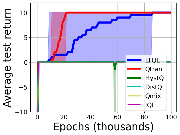
In this experiment we use a tabular representation in an environment that is stochastic and episodic. The environment is a linear grid with 4 positions and 2 agents. At the beginning of the episode, the agents are initialized in the far right. Agent 1 cannot move and has 2 actions (push button or not push), while agent 2 has 3 actions (stay, move left or move right). If agent 2 is located in the far left and chooses to stay while agent 2 chooses push, the team receives a reward. If the button is pushed while agent 2 is moving left the team receives a reward. This negative reward is also obtained if agent 2 stays still in the leftmost position and agent 1 does not push the button. All rewards are subject to additive Gaussian noise with mean 0 and standard deviation equal to 1. Furthermore if agent 2 tries to move beyond an edge (left or right), it stays in place and the team receives a Gaussian reward with mean and standard deviation equal to . The episode finishes after 5 timesteps or if the team gets the reward (whichever happens first). We ran the simulation times with different seeds. Figure 1(b) shows the average test return44 4 The average test return is the return following a greedy policy averaged over games. (without the added noise) of IQL, LTQL, HystQ, DistQ, Qmix and Qtran. As can be seen, LTQL and Qtran are the only algorithms capable of learning optimal team policies. In appendix 6.6 we specify the hyperparameters and include the learning curves of the -functions along with a discussion on the performance of each algorithm.
5.3 Cowboy Bull Game
In this experiment we use a more complex environment, a challenging predator-prey type game with partial observability, in which 4 cowboys try to catch a bull (see figure 1(c)). The position of all players is a continuous variable (and hence the state space is continuous). The space is unbounded and the bull can move faster than the cowboys. The bull follows a fixed stochastic policy, which is handcrafted to mimic natural behavior and evade capture. Due to the unbounded space and the fact that the bull moves faster than the cowboys, it cannot be captured unless all agents develop a coordinated strategy (the bull can only be caught if the agents first surround it and then evenly close in). The task is episodic and ends after 75 timesteps or when the bull is caught. Each agent has 5 actions (the four moves plus stay). When the bull is caught a reward is obtained and the team also receives a small penalty () for every agent that moves. Note that due to the reward structure there is a very easily attainable Nash equilibrium, which is for every agent to stay still (since in this way they do not incur in the penalties associated with movement). Figure 1(d) shows the test win percentage55 5 Percentage of games, out of 50, in which the team succeeds to catch the bull following a greedy policy. and figure 1(e) shows the average test return for IQL, LTQL, HystQ, Qmix and Qtran. The best performing algorithm is LTQL. HystQ learns a policy that catches the bull of the times, although it fails at obtaining returns higher than zero. IQL fails because the agents quickly converge to the policy of never moving (to avoid incurring in the negative rewards associated with movement). We believe that the poor performance of Qmix in this task is a consequence of its limited representation capacity due to its monotonic factoring model. Qtran fails in this complex scenario, which is in agreement with results reported in [Rashid et al., 2020] where Qtran also shows poor performance in the Starcraft multi-agent challenge (SMAC) [Samvelyan et al., 2019]. In the appendix we provide all hyperparameters and implementation details, we detail the bull’s policy and the observation function. All code66 6 Code is also available at https://github.com/lcassano/Logical-Team-Q-Learning-paper., a pre-trained model and a video of the policy learned by LTQL are included as supplementary material.
6 CONCLUDING REMARKS
In this article we have introduced Logical Team Q-Learning, which has the desirable properties mentioned in the introduction. LTQL does not impose constraints on the learned individual -functions and hence it can solve environments where state of the art algorithms like Qmix and Qtran fail. The algorithm fits in the centralized training and decentralized execution paradigm. It can also be implemented in a fully distributed manner in situations where all agents have access to each others’ observations and actions.
References
- [Bellemare et al., 2013] Bellemare, M. G., Naddaf, Y., Veness, J., and Bowling, M. (2013). The arcade learning environment: An evaluation platform for general agents. Journal of Artificial Intelligence Research, 47:253–279.
- [Cassano et al., 2019] Cassano, L., Alghunaim, S. A., and Sayed, A. H. (2019). Team policy learning for multi-agent reinforcement learning. In IEEE International Conference on Acoustics, Speech and Signal Processing (ICASSP), pages 3062–3066.
- [Claus and Boutilier, 1998] Claus, C. and Boutilier, C. (1998). The dynamics of reinforcement learning in cooperative multiagent systems. AAAI/IAAI, 1998(746-752):2.
- [Duchi et al., 2011] Duchi, J., Hazan, E., and Singer, Y. (2011). Adaptive subgradient methods for online learning and stochastic optimization. Journal of Machine Learning Research, pages 2121–2159.
- [Foerster et al., 2017] Foerster, J., Nardelli, N., Farquhar, G., Afouras, T., Torr, P. H., Kohli, P., and Whiteson, S. (2017). Stabilising experience replay for deep multi-agent reinforcement learning. In Proceedings International Conference on Machine Learning, pages 1146–1155.
- [Foerster et al., 2018] Foerster, J. N., Farquhar, G., Afouras, T., Nardelli, N., and Whiteson, S. (2018). Counterfactual multi-agent policy gradients. In AAAI Conference on Artificial Intelligence.
- [Guestrin et al., 2002a] Guestrin, C., Koller, D., and Parr, R. (2002a). Multiagent planning with factored MDPs. In Advances in neural information processing systems, pages 1523–1530.
- [Guestrin et al., 2002b] Guestrin, C., Lagoudakis, M., and Parr, R. (2002b). Coordinated reinforcement learning. In ICML, volume 2, pages 227–234.
- [Gupta et al., 2017] Gupta, J. K., Egorov, M., and Kochenderfer, M. (2017). Cooperative multi-agent control using deep reinforcement learning. In International Conference on Autonomous Agents and Multiagent Systems, pages 66–83, Sao Paulo, Brazil.
- [Hausknecht and Stone, 2015] Hausknecht, M. and Stone, P. (2015). Deep recurrent Q-learning for partially observable mdps. In AAAI Fall Symposium on Sequential Decision Making for Intelligent Agents, Virginia, USA.
- [Hochreiter and Schmidhuber, 1997] Hochreiter, S. and Schmidhuber, J. (1997). Long short-term memory. Neural computation, 9(8):1735–1780.
- [Kingma and Ba, 2014] Kingma, D. P. and Ba, J. (2014). Adam: A method for stochastic optimization. arXiv:1412.6980.
- [Kok and Vlassis, 2004] Kok, J. R. and Vlassis, N. (2004). Sparse cooperative Q-learning. In Proceedings International Conference on Machine Learning, page 61.
- [Lauer and Riedmiller, 2000] Lauer, M. and Riedmiller, M. (2000). An algorithm for distributed reinforcement learning in cooperative multi-agent systems. In Proc. International Conference on Machine Learning (ICML), pages 535–542, Palo Alto, USA.
- [Lin, 1992] Lin, L.-J. (1992). Self-improving reactive agents based on reinforcement learning, planning and teaching. Machine Learning, 8(3-4):293–321.
- [Littman, 2001] Littman, M. L. (2001). Value-function reinforcement learning in markov games. Cognitive Systems Research, 2(1):55–66.
- [Matignon et al., 2007] Matignon, L., Laurent, G., and Le Fort-Piat, N. (2007). Hysteretic Q-learning: an algorithm for decentralized reinforcement learning in cooperative multi-agent teams. In Proc. IEEE/RSJ International Conference on Intelligent Robots and Systems, pages 64–69, San Diego, USA.
- [Mnih et al., 2013] Mnih, V., Kavukcuoglu, K., Silver, D., Graves, A., Antonoglou, I., Wierstra, D., and Riedmiller, M. (2013). Playing Atari with deep reinforcement learning. arXiv:1312.5602.
- [Oliehoek et al., 2016] Oliehoek, F. A., Amato, C., et al. (2016). A Concise Introduction to Decentralized POMDPs, volume 1. Springer.
- [Omidshafiei et al., 2017] Omidshafiei, S., Pazis, J., Amato, C., How, J. P., and Vian, J. (2017). Deep decentralized multi-task multi-agent reinforcement learning under partial observability. In Proceedings International Conference on Machine Learning, pages 2681–2690.
- [Rashid et al., 2020] Rashid, T., Samvelyan, M., De Witt, C. S., Farquhar, G., Foerster, J., and Whiteson, S. (2020). Monotonic value function factorisation for deep multi-agent reinforcement learning. Journal of Machine Learning Research, 21(178):1–51.
- [Rashid et al., 2018] Rashid, T., Samvelyan, M., Schroeder, C., Farquhar, G., Foerster, J., and Whiteson, S. (2018). Qmix: Monotonic value function factorisation for deep multi-agent reinforcement learning. In Proceedings of the International Conference on Machine Learning, pages 4295–4304.
- [Samvelyan et al., 2019] Samvelyan, M., Rashid, T., Schroeder de Witt, C., Farquhar, G., Nardelli, N., Rudner, T. G. J., Hung, C.-M., Torr, P. H. S., Foerster, J., and Whiteson, S. (2019). The StarCraft Multi-Agent Challenge. In Proceedings of the International Conference on Autonomous Agents and MultiAgent Systems, pages 2186–2188.
- [Son et al., 2019] Son, K., Kim, D., Kang, W. J., Hostallero, D. E., and Yi, Y. (2019). Qtran: Learning to factorize with transformation for cooperative multi-agent reinforcement learning. In International Conference on Machine Learning, pages 5887–5896.
- [Sunehag et al., 2018] Sunehag, P., Lever, G., Gruslys, A., Czarnecki, W. M., Zambaldi, V., Jaderberg, M., Lanctot, M., Sonnerat, N., Leibo, J. Z., Tuyls, K., et al. (2018). Value-decomposition networks for cooperative multi-agent learning based on team reward. In Proceedings International Conference on Autonomous Agents and Multiagent Systems, pages 2085–2087.
- [Sutton and Barto, 1998] Sutton, R. S. and Barto, A. G. (1998). Reinforcement Learning: An Introduction. MIT Press.
- [Tampuu et al., 2017] Tampuu, A., Matiisen, T., Kodelja, D., Kuzovkin, I., Korjus, K., Aru, J., Aru, J., and Vicente, R. (2017). Multiagent cooperation and competition with deep reinforcement learning. PloS one, 12(4).
- [Tan, 1993] Tan, M. (1993). Multi-agent reinforcement learning: Independent vs. cooperative agents. In Proceedings International Conference on Machine Learning, pages 330–337.
- [Tesauro, 2004] Tesauro, G. (2004). Extending Q-learning to general adaptive multi-agent systems. In Proc. Advances in Neural Information Processing Systems, pages 871–878, Vancouver, Canada.
- [Uspensky, 1937] Uspensky, J. V. (1937). Introduction to mathematical probability. McGraw-Hill, New York.
- [Wang and Sandholm, 2003] Wang, X. and Sandholm, T. (2003). Reinforcement learning to play an optimal nash equilibrium in team markov games. In Proc. Advances in Neural Information Processing Systems, pages 1603–1610, Vancouver, Canada.
- [Watkins and Dayan, 1992] Watkins, C. and Dayan, P. (1992). Q-learning. Machine Learning, 8(3-4):279–292.
- [Zhang et al., 2019] Zhang, K., Yang, Z., and Başar, T. (2019). Multi-agent reinforcement learning: A selective overview of theories and algorithms. arXiv:1911.10635.
- [Zhang et al., 2018] Zhang, K., Yang, Z., Liu, H., Zhang, T., and Başar, T. (2018). Fully decentralized multi-agent reinforcement learning with networked agents. In Proceedings of the International Conference on Machine Learning, pages 5872–5881.
Appendix
6.1 Proof of proposition 3
Consider the matrix game with two agents, each of which has two actions () and the following reward structure:
| Agent | |||
|---|---|---|---|
| Agent | |||
For this case , , , , and are given by:
Notice that as expected, satisfies (3c). However, note that (3c) is also satisfied by the following function which is different from .
| (34) |
Notice further that the team policy obtained by choosing actions in a greedy fashion with respect to constitutes a sub-optimal Nash equilibrium.
6.2 Proof of Lemma 1
We start defining:
| (35) | ||||
| (36) |
where . We recall that to simplify notation we defined . The first part of the proof consists in upper bounding any sequence of the form , where for all . Applying operator to we get:
| (37) |
Therefore, for any . Applying operator we get:
| (38) | ||||
| (39) | ||||
| (40) |
Further application of we get:
| (41) |
Therefore, we conclude that . More generally, we can write:
| (42) |
where we define to be the total number of times that operator is applied. Notice that if operator is applied times, is a random variable that follows a binomial distribution with total samples and probability . Therefore, we get:
| (43) |
To ensure that we need:
| (44) |
Since follows a binomial distribution we get:
| (45) |
Therefore we can conclude that:
| (46) | ||||
| (47) |
Noting that by construction for all , we get that:
| (48) |
For the special case where we can bound the cumulative distribution function of the binomial distribution using Hoeffding’s bound:
| (49) |
which concludes the proof.
6.3 Proof of Lemma 2
We start stating the following auxiliary lemma.
Lemma 3.
If then it holds that for all .
Proof.
We start noting that if then and .
| (50) | ||||
| (51) |
where in and we used the fact that . Since it holds that and it immediately follows that for all .
We follow by noting that applying operator times to we get:
| (52) | ||||
| (53) |
where in we used from lemma 3. If , we get:
| (54) | ||||
| (55) |
Lemma 4.
If and is small enough, then it holds that for all .
Proof.
Assume satisfies the following relation:
| (56) |
We clarify that the term in between parenthesis in the r.h.s. of relation (56) is the difference between the optimal -value and the second highest -value for state . Note that if then it trivially follows that , for the case of we get:
| (57) |
Using equation (3a) and the fact that it follows:
| (58) | ||||
| (59) | ||||
| (60) |
where in we used condition (56). Combining equations (57) through (60) we get:
| (61) |
Combining equation (61) with the fact that we get:
| (62) |
which completes the proof.
Lemma 5.
For any , and , it holds that as long as the sequence of operators includes at least consecutive ’s. Where is given by:
| (63) |
Proof.
Notice that the probability of applying operator at least consecutive times when operator is applied times, is the same as the probability of obtaining at least consecutive heads when a biased coin (with probability of head ) is tossed times. This problem has been extensively studied and the result is available in the literature. We state the following useful result from [Uspensky, 1937]:
Lemma 6.
[Uspensky, 1937]: If a biased coin (with probability of head being ) is tossed times, the probability of having a sequence of at least consecutive heads is given by:
| (64) | ||||
| (65) |
Furthermore, if the probability can be lower bounded as follows:
| (66) |
where .
6.4 Tabular Logical Team Q-Learning
In the particular case where the MDP is deterministic (and hence ) the tabular version of Logical Team Q-learning is given by algorithm 2.
If algorithm 2 were applied to a stochastic MDP, due to condition , it would be subject to bias, which would propagate through bootstrapping and hence could compromise its performance. This can be solved by having a second unbiased estimate that is updated only when is satisfied and use this unbiased estimate to bootstrap. The resulting algorithm is shown in algorithm 3.
6.5 Matrix game additional results
We start specifying the hyperparameters. For IQL, DistQ, LTQL and Qtran we used a step-size equal to . The parameter for LTQL is equal to . The mixing network in Qmix has hidden layers with units each, the nonlinearity used was the ELu and the step-size used was (we had to make it smaller than the others to make the SGD optimizer converge). We finally remark that due to the use of a NN in Qmix we had to train this algorithm with times more games (notice the x-axis in figure 2).
In figure 2 we show the convergence curves for IQL 2(a), DistQ 2(b), LTQL 2(c)-2(f), Qmix 2(g) and Qtran 2(h). Figures 2(c) and 2(d) correspond to the deterministic (algorithm 2) and general version (algorithm 3) of LTQL, respectively. Figures 2(e) and 2(f) also show curves for LTQL but use different seeds and show that this algorithm can converge to either of the two following set of factored -functions:
| (71) |
One interesting fact to note is that the suboptimal values of (in figures 2(c) and 2(e)) do not converge while the same values do converge in the case of . The reason for this is that there is a parallel between including the unbiased estimate in the RL algorithm and including an application of operator at the end of the dynamic programming procedure described in theorem 1. The proof of the theorem shows that if such operator is not included, only the optimal values of the estimates generated by Logical Team Q-learning converge to , while the values corresponding to suboptimal actions oscillate in the region between and (which is what happens when the unbiased estimate is not used in algorithm 2). Note that in the case of algorithm 3 where the unbiased estimate is included all values converges to for all actions, not just the optimal ones (this is equivalent to including the operator after in the dynamic programming setting).


Below we show the joint values generated by Qmix’s mixing network.
| Agent | ||||
|---|---|---|---|---|
| Agent 1 | ||||
Code is available at https://github.com/lcassano/Logical-Team-Q-Learning-paper.
6.6 Stochastic TMDP additional results
In this environment agents rely on the following observations. The observation corresponding to agent 1 is a vector with two binary elements: the first one indicates whether or not agent 2 is in the leftmost position, and the second element indicates whether or not there is enough time for agent 2 to reach the leftmost position. The observation corresponding to agent 2 is a vector with two elements: the first one is the number of the position it occupies and the second one is the same as agent 1 (whether there is enough time to reach the leftmost position).
All algorithms are implemented in an on-line manner with no replay buffer. -greedy exploration with a decaying schedule is used in all cases (). The step-size used is and the smaller step-size for HystQ is , in the case of Qmix we used to guarantee stability. The parameter for LTQL is equal to .
Figures 3 show the estimated -values for LTQL corresponding to 4 different observations at the 4 positions. Note that in all figures the optimum action has the highest value and correctly estimates the return corresponding to the optimal team policy ().


Figures 4 show the learning curves for IQL. Note that IQL fails at this environment because it has no mechanism to discard the penalty incurred due to moving to the left when agent 1 presses the button due to exploration.


Figures 5 show the learning curves for DistQ. The reason that this algorithm cannot solve this environment is that it severely overestimates the value of choosing to move to the right whilst on the rightmost position. It is well known that this is a consequence of the fact that DistQ only performs updates that increase the estimates of the -values combined with the stochastic reward received when agent 2 “stumbles” against the right edge.


Figures 6 show the learning curves for HystQ. This algorithm cannot solve this environment because it has two issues and the way to solve one makes the other worse. More specifically, one can be solved by increasing the smaller step-size, while the other needs to decrease it. The first issue is the same one that affects DistQ, i.e., the overestimation of the move right action in the rightmost position. Note that this can be ameliorated by increasing the small step-size. The second issue is the penalty incurred due to moving to the left when agent 1 presses the button. This can be ameliorated by decreasing the small step-size. The fact that there is no intermediate value for the small step-size to solve both issues is the reason that this algorithm cannot solve this environment.


Figures 7 show the learning curves for Qmix. Qmix fails at this task due to the fact that its monotonic factoring assumption is not satisfied at this task. The architecture used is as follows: we used tabular representation for the individual functions, and for the mixing and hypernetworks we used the architecture specified in [Rashid et al., 2020]. More specifically, the mixing network is composed of two hidden layers (with units each) with ELu nonlinearities in the first layer while the second layer is linear. The hypernetworks that output the weights of the mixing network consist of two layers with nonlinearities followed by an activation function that takes the absolute value to ensure that the mixing network weights are non-negative. The bias of the first mixing layer is produced by a network with a unique linear layer and the other bias is produced by a two layer hypernetwork with a nonlinearity. All hypernetwork layers are fully connected and have units.


Figures 8 show the learning curves for Qtran. Qtran succeeds at this task. However, it is important to remark that this is a tabular implementation of Qtran (an algorithm designed to be used in conjuntion with NNs in complex environment), where the algorithm estimates the full joint q-function in tabular form, which is not scalable and defeats the purpose of learning factored q-functions.


All code is available at https://github.com/lcassano/Logical-Team-Q-Learning-paper.
6.7 Cowboy bull game additional results
The bull’s policy is given by the pseudocode shown in algorithm 4.
We now specify the hyperparameters for Logical Team Q-learning. All NN’s have two hidden layers with units and ReLu nonlinearities. However, for each -network, instead of having one network with outputs, we have networks each with output (one for each action). At every epoch the agent collects data by playing full games and then performs gradient backpropagation steps. Half of the games are played greedily and the other half use a Boltzmann policy with temperature that decays according to the following schedule . We use this behavior policy to ensure that there are sufficient transitions that satisfy condition and that also there are transitions that satisfy . The target networks are updated every backprop steps. The capacity of the replay buffer is transitions, the mini-batch size is 1024, , we use a discount factor equal to and optimize the networks using the Adam optimizer with initial step-size .
The hyperparameters of the HystQ implementation are the same as those of LTQL, the ratio of the two step-sizes used by HystQ is . To run IQL we used the implementation of HystQ with the ratio of the two step-sizes set to .
The architecture used by Qmix is the one suggested in [Rashid et al., 2020] with the exception that, for fairness, the individual -networks used the same architecture as the ones used by the other algorithms (i.e., networks with a unique output as opposed to network with outputs). All hidden layers of the hypernetworks as well the mixing network have units. In this case we did backprop iterations per epoch and the target network update period is . We use a batch size of , a discount factor equal to and optimize the networks with the Adam optimizer with initial step-size . In this case the behavior policy is always Boltzmann with the following annealing schedule for the temperature parameter .
The Qtran-base variant was implemented. The individual -networks have the same architecture used by the other algorithms. The joint -network has two hidden layers with units each, the input of this network is the global state concatenated with the agents’ actions with one hot encoding. The value function network has only one hidden layer with units and its input is the global state. The target networks are updated every backprop steps. The capacity of the replay buffer is transitions, the mini-batch size is 1024, we use a discount factor equal to and optimize the networks using the Adam optimizer with initial step-size .
The batch size, Boltzmann temperature value, learning step-size and target update period were chosen by grid search.
All implementations use TensorFlow 2. The code is available at https://github.com/lcassano/Logical-Team-Q-Learning-paper. Running one seed for one agent takes approximately 12 hours in our hardware (2017 iMac with 3.8 GHz Intel Core i5 and 16GB of RAM).