Joint Performance Analysis of Ages of Information in a Multi-source Pushout Server

Yukang Jiang Naoto Miyoshi Thanks: Y. Jiang and N. Miyoshi are with Department of Mathematical and Computing Science, Tokyo Institute of Technology, Tokyo, Japan. E-mail: miyoshi@is.titech.ac.jp. Thanks: The support of the Japan Society for the Promotion of Science˜(JSPS) Grant-in-Aid for Scientific Research (C) 19K11838 is gratefully acknowledged.

Abstract

Age of information (AoI) has been widely accepted as a measure quantifying freshness of status information in real-time status update systems. In many of such systems, multiple sources share a limited network resource and therefore the AoIs defined for the individual sources should be correlated with each other. However, there are not found any results studying the correlation of two or more AoIs in a status update system with multiple sources. In this work, we consider a multi-source system sharing a common service facility and provide a framework to investigate joint performance of the multiple AoIs. We then apply our framework to a simple pushout server with multiple sources and derive a closed-form formula of the joint Laplace transform of the AoIs in the case with independent M/G inputs. We further show some properties of the correlation coefficient of AoIs in the two-source system.

Index Terms:

Age of information, multi-source status update systems, joint Laplace transform, multi-source pushout server, correlation coefficient, Palm calculus, stationary framework.

I Introduction

Freshness of status information is crucial in real-time status update systems seen, for example, in weather reports, autonomous driving, stock market trading and so on. Age of information (AoI) has been widely accepted in this decade as a measure quantifying the freshness of information in status update systems where information sources transmit packets containing status updates to destination monitors through a communication network. Specifically, the AoI is defined as the elapsed time since the information currently displayed on a monitor is generated and timestamped at the source. In many of such systems, multiple sources share a limited network resource and therefore the AoIs defined for the individual sources should be correlated with each other. However, to the best of the knowledge of the authors, there are no results studying the correlation of two or more AoIs in a status update system with multiple sources (except for the first author’s preliminary work [1]). To investigate the correlation is essential when, for example, we consider a nonlinear penalty function of multiple AoIs. In this work, we consider a multi-source system sharing a common service facility and provide a framework to investigate joint performance of the AoIs defined for the individual sources.

I-A Related work

Since the advent in [2, 3], a large amount of literature has emerged on development of the AoI concept due to its importance and availability in a wide range of information communication systems. A complete review falls out of the reach of this paper and we only highlight some relevant results to ours. Interested readers are referred to recent monographs [4, 5] and references therein.

The AoI was first introduced in [2] in the context of vehicular networks and queueing-theoretic technique was applied in [3] to analyze the mean AoI under the ergodicity assumption. These results were then extended to various multi-source systems in [6, 7, 8]. A more tractable metric, peak AoI (PAoI)—the AoI immediately before an update, was introduced in [9, 10], which characterized not only the mean but also the probability distribution of the PAoI for various queueing systems under the ergodicity. Not only the mean, expected nonlinear functions of the AoI were examined in [11, 12].

In the early stage of the development, they assumed that time intervals of packet generations and their service times are either exponentially distributed or deterministic; that is, they considered M/M, M/D or D/M inputs in the queueing notation. Recently, some researchers have challenged to incorporate more general probability distributions. In [13], gamma distributed service times were assumed for Poisson arrival systems and [14, 15] considered more general service time distributions in multi-source systems with independent Poisson arrivals; that is, they treated independent M/G input processes. Furthermore, [16, 17, 18] studied more general frameworks of packet arrival and service time processes and derived general formulas satisfied by the stationary distribution and its Laplace transform of the AoI, where [16, 17] adopted the technique of sample path analysis while [18] worked based on the Palm calculus within the stationary framework (see, e.g., [19] for the Palm calculus). However, there are no results confronting joint performance of multiple AoIs in multi-source systems within general frameworks.

I-B Contribution

In this paper, we consider a multi-source system sharing a service facility as in [6, 7, 8, 14, 15] and provide a framework to investigate joint performance of the AoIs defined for the individual sources. We first consider a general multi-source system, where the time sequence representing service completions (and status updates) follows a stationary point process on the real line, and derive a formula satisfied by the joint Laplace transform of the stationary AoIs. A tool for our analysis is the Palm calculus within the stationary framework as in [18], where we do not require the ergodic assumption but, once the ergodicity is assumed, we can obtain the same results as those from the sample path analysis by the ergodic theorem. Our formula is so general and is applicable to many multi-source systems. We then apply this formula to a simple pushout server, where the system has a single server and each generated packet is immediately started for service without waiting; that is, the ongoing service of another packet (if any) is interrupted and replaced by the new one. In the case with independent M/G input processes, we derive a closed-form formula of the joint Laplace transform of the AoIs. Furthermore, we reveal some properties of the correlation coefficient of the AoIs in the two-source system.

I-C Organization

The rest of the paper is organized as follows. In the next section, we describe a general multi-source system and derive a formula satisfied by the joint Laplace transform of the multiple AoIs. We also provide a formula for a single-source system, which corresponds to the review of the results in [16, 17] within our stationary framework. In Section III, we apply our formula to a multi-source pushout server. We first confirm in III-A that our multi-source pushout server is definitely within our framework and then derive a closed-form formula of the joint Laplace transform of the AoIs in the case with independent M/G inputs in III-B. Some properties of the correlation coefficient of the AoIs in the two-source system are revealed in III-C. These properties of the correlation coefficient are confirmed through numerical experiments in Section IV. Finally, concluding remarks and future work are discussed in Section V.

II General multi-source system

In this section, we consider a general multi-source single-server system. There are $K$ ( $\in\mathbb{N}=\{1,2,\ldots\}$ ) sources generating packets with different kinds of status information and each source has its dedicated monitor. The set of the sources is denoted by $\mathcal{K}=\{1,2,\ldots,K\}$ . The system has a single server and, after a packet from source $k\in\mathcal{K}$ is processed by the server, the status information in the packet is immediately displayed on monitor $k$ . We note that not all packets are completed for service and some may be discarded and lost (due to buffer overflows, packet deadlines or pushouts). We, for the moment, ignore such lost packets and focus on those being completed for service.

Let $\Psi$ denote a point process on $\mathbb{R}=(-\infty,\infty)$ counting the times at each of which the service of a packet is completed and the status information on one of the monitors is updated, and let $\{U_{n}\}_{n\in\mathbb{Z}}$ denote the corresponding time sequence, where $\mathbb{Z}=\{\cdots,-1,0,1,2,\ldots\}$ . For $n\in\mathbb{Z}$ , let $C_{n}$ and $D_{n}$ denote respectively the source and the delay of the packet whose service is completed at $U_{n}$ ; that is, the status information updated at $U_{n}$ is generated and timestamped at $U_{n}-D_{n}$ by source $C_{n}$ . For each $k\in\mathcal{K}$ , let $\Psi_{k}$ denote a sub-process of $\Psi$ counting the times of service completions of source $k$ packets; that is,

\Psi_{k}(B)=\sum_{n\in\mathbb{Z}}\bm{1}_{\{k\}}(C_{n})\bm{1}_{B}(U_{n}),\quad B\in\mathcal{B}(\mathbb{R}),

(1)

where $\bm{1}_{E}$ denotes the indicator function of a set $E$ . Clearly, $\Psi_{k}$ , $k\in\mathcal{K}$ , are mutually disjoint and satisfy $\Psi=\sum_{k=1}^{K}\Psi_{k}$ . We impose the following assumption on the marked point process $\Psi_{C,D}$ corresponding to $\{(U_{n},C_{n},D_{n})\}_{n\in\mathbb{Z}}$ .

Assumption 1

1.

The point process $\Psi$ is simple almost surely in a probability $\mathbb{P}$ ( $\mathbb{P}$ -a.s.), where the rule of subscripts is such that $\cdots<U_{-1}<U_{0}\leq 0<U_{1}<\cdots$ conventionally (see, e.g., [19]).
2.

The marked point process $\Psi_{C,D}$ is stationary in $\mathbb{P}$ with mark space $\mathcal{K}\times[0,\infty)$ .
3.

The point process $\Psi$ has positive and finite intensity $\lambda_{\Psi}=\mathbb{E}[\Psi(0,1]]$ , where $\mathbb{E}$ denotes the expectation with respect to $\mathbb{P}$ .
4.

$\mathbb{P}_{\Psi}^{0}(C_{0}=k)>0$ for all $k\in\mathcal{K}$ , where $\mathbb{P}_{\Psi}^{0}$ denotes the Palm probability for $\Psi$ .
5.

$\mathbb{P}_{\Psi_{k}}^{0}(D_{0}<\infty)=1$ for all $k\in\mathcal{K}$ , where $\mathbb{P}_{\Psi_{k}}^{0}$ denotes the Palm probability for $\Psi_{k}$ .

Note that the Palm probability $\mathbb{P}_{\Psi}^{0}$ is well defined under Assumptions 1-2) and 3) (see [19]) and that $\mathbb{P}_{\Psi}^{0}(U_{0}=0)=1$ . Furthermore, under Assumption 1-2), $\{(C_{n},D_{n})\}_{n\in\mathbb{Z}}$ is stationary in $\mathbb{P}_{\Psi}^{0}$ . Assumption 1-4) does not restrict us since we can redefine $\mathcal{K}$ by $\mathcal{K}\setminus\{k\}$ if $\mathbb{P}_{\Psi}^{0}(C_{0}=k)=0$ for some $k\in\mathcal{K}$ . The intensity $\lambda_{\Psi_{k}}$ of the sub-process $\Psi_{k}$ is given by $\lambda_{\Psi_{k}}=\lambda_{\Psi}\,\mathbb{P}_{\Psi}^{0}(C_{0}=k)$ for each $k\in\mathcal{K}$ , so that the Palm probability $\mathbb{P}_{\Psi_{k}}^{0}$ is also well defined under 1-2)–4) and satisfies $\mathbb{P}_{\Psi_{k}}^{0}(\cdot)=\mathbb{P}_{\Psi}^{0}(\cdot\mid C_{0}=k)$ . Let $\{U_{k,n}\}_{n\in\mathbb{Z}}$ , $k\in\mathcal{K}$ , denote the time sequence corresponding to $\Psi_{k}$ satisfying $\cdots<U_{k,-1}<U_{k,0}\leq 0<U_{k,1}<\cdots$ , and let also $D_{k,n}$ denote the delay of the source $k$ packet whose service is completed at $U_{k,n}$ (note that $D_{k,0}=D_{0}$ $\mathbb{P}_{\Psi_{k}}^{0}$ -a.s.). Then, the AoI process $\{A_{k}(t)\}_{t\in\mathbb{R}}$ for source $k\in\mathcal{K}$ is defined as (see [7, 8] for AoI in multi-source systems)

A_{k}(t)=D_{k,n}+t-U_{k,n},\quad t\in[U_{k,n},U_{k,n+1}),\;n\in\mathbb{Z}.

(2)

This definition indicates that the AoI of source $k$ represents the elapsed time since the information currently displayed on monitor $k$ is generated and timestamped; that is, it is set to the delay of a source $k$ packet at its service completion time and increases linearly until the status information from source $k$ is next updated.

Lemma 1

For each $k\in\mathcal{K}$ , the marked point process $\Psi_{k,D}$ corresponding to $\{(U_{k,n},\,D_{k,n})\}_{n\in\mathbb{Z}}$ and also the AoI processes $\{A_{k}(t)\}_{t\in\mathbb{R}}$ are jointly stationary with the marked point process $\Psi_{C,D}$ under Assumption 1. Furthermore, $A_{k}(0)$ is $\mathbb{P}$ -a.s. finite under the same assumption.

Proof:

The proof relies on a technical discussion within the stationary framework and is given in Appendix A. ∎

While the AoI just after an update is equal to the delay $D_{k,n}=A(U_{k,n})$ , that just before an update is called the PAoI (see [9, 10]); that is, for each $k\in\mathcal{K}$ , the sequence $\{P_{k,n}\}_{n\in\mathbb{Z}}$ of PAoIs is defined as $P_{k,n}=A(U_{k,n}-)$ , $n\in\mathbb{Z}$ , and is also stationary in $\mathbb{P}_{\Psi_{k}}^{0}$ . Prior to the joint performance analysis of $A_{1}(t),\ldots,A_{K}(t)$ , $t\in\mathbb{R}$ , we review the results of [16, 17] for a single-source single-server system within our stationary framework, which is also useful in the marginal performance analysis of multi-source systems.

Proposition 1 (Cf. [16, 17])

Consider a single-source system satisfying Assumption 1 with $K=1$ , where $A(t)=A_{1}(t)$ , $D_{n}=D_{1,n}$ and $P_{n}=P_{1,n}$ in (2). Then, the stationary distribution of the AoI satisfies

\mathbb{P}(A(0)\leq x)=\lambda_{\Psi}\int_{0}^{x}\bigl(\mathbb{P}_{\Psi}^{0}(P_{0}>u)-\mathbb{P}_{\Psi}^{0}(D_{0}>u)\bigr)\,\mathrm{d}u,\quad x\geq 0.

(3)

Let $\mathcal{L}_{A}(s)=\mathbb{E}[e^{-sA(0)}]$ , $\mathcal{L}_{D}(s)=\mathbb{E}_{\Psi}^{0}[e^{-sD_{0}}]$ and $\mathcal{L}_{P}(s)=\mathbb{E}_{\Psi}^{0}[e^{-sP_{0}}]$ , $s\in\mathbb{R}$ , denote the Laplace transforms of $A(0)$ , $D_{0}$ and $P_{0}$ , respectively, where $\mathbb{E}_{\Psi}^{0}$ denotes the expectation with respect to the Palm probability $\mathbb{P}_{\Psi}^{0}$ . Then, the following relation holds;

s\,\mathcal{L}_{A}(s)=\lambda_{\Psi}\,\bigl(\mathcal{L}_{D}(s)-\mathcal{L}_{P}(s)\bigr),

(4)

for $s\in\mathbb{R}$ such that the Laplace transforms on both the sides exist.

Proof:

Applying the Palm inversion formula (see [19, p. 20]),

	$\displaystyle\mathbb{P}(A(0)\leq x)$	$\displaystyle=\lambda_{\Psi}\,\mathbb{E}_{\Psi}^{0}\biggl[\int_{[0,\,U_{1})}\bm{1}_{[0,\,x]}(A(t))\,\mathrm{d}t\biggr]$
		$\displaystyle=\lambda_{\Psi}\,\mathbb{E}_{\Psi}^{0}\biggl[\int_{[D_{0},\,P_{1})}\bm{1}_{[0,\,x]}(u)\,\mathrm{d}u\biggr]$
		$\displaystyle=\lambda_{\Psi}\,\mathbb{E}_{\Psi}^{0}[P_{1}\wedge x-D_{0}\wedge x],\quad x\geq 0,$

where $a\wedge b=\min(a,b)$ for $a,b\in\mathbb{R}$ and the second equality follows from (2); that is, $A(t)$ increases linearly from $D_{0}$ to $P_{1}$ for $t\in[U_{0},U_{1})$ . The last expression above immediately derives (3) since $P_{1}$ is distributionally equal to $P_{0}$ in $\mathbb{P}_{\Psi}^{0}$ . The formula (4) is obtained from (3) as

	$\displaystyle\mathcal{L}_{A}(s)$	$\displaystyle=\int_{0}^{\infty}e^{-sx}\,\mathbb{P}(A(0)\in\mathrm{d}x)$
		$\displaystyle=\lambda_{\Psi}\int_{0}^{\infty}e^{-sx}\,\bigl(\mathbb{P}_{\Psi}^{0}(P_{0}>x)-\mathbb{P}_{\Psi}^{0}(D_{0}>x)\bigr)\,\mathrm{d}x,$

using $\mathbb{E}[e^{-sX}]=1-s\int_{0}^{\infty}e^{-sx}\,\mathbb{P}(X>x)\,\mathrm{d}x$ for a random variable $X$ and $s\in\mathbb{R}$ such that $\mathbb{E}[e^{-sX}]$ is finite. ∎

Remark 1

Formulas (3) and (4) respectively correspond to the results of Theorem 14 (i) and (ii) in [17]. As opposed to [16, 17], however, Proposition 1 does not require the ergodicity of $\{(D_{n},P_{n})\}_{n\in\mathbb{Z}}$ . These formulas suggest that we can obtain the stationary distribution of the AoI and the corresponding Laplace transform once the stationary distributions of the delay and PAoI are available. The formula (3) also implies that the stationary distribution of the AoI has the density function $\lambda_{\Psi}\,\bigl(\mathbb{P}_{\Psi}^{0}(P_{0}>x)-\mathbb{P}_{\Psi}^{0}(D_{0}>x)\bigr)$ , $x\geq 0$ . Taking $x\to\infty$ in (3), we have $\mathbb{E}_{\Psi}^{0}[P_{0}]=\mathbb{E}_{\Psi}^{0}[D_{0}]+1/\lambda_{\Psi}$ , which intuitively makes sense since a PAoI is the sum of a delay and its subsequent interdeparture time (see (2)).

Proposition 1 can be applied to the marginal distribution of each AoI in a system with $K\geq 2$ .

Corollary 1

For a system with $K$ sources satisfying Assumption 1, the marginal stationary distribution of the AoI for source $k\in\mathcal{K}$ satisfies

\mathbb{P}(A_{k}(0)\leq x)=\lambda_{\Psi_{k}}\int_{0}^{x}\bigl(\mathbb{P}_{\Psi_{k}}^{0}(P_{k,0}>u)-\mathbb{P}_{\Psi_{k}}^{0}(D_{k,0}>u)\bigr)\,\mathrm{d}u,\quad x\geq 0.

(5)

Let $\mathcal{L}_{A_{k}}(s)=\mathbb{E}[e^{-sA_{k}(0)}]$ , $\mathcal{L}_{D_{k}}(s)=\mathbb{E}_{\Psi_{k}}^{0}[e^{-sD_{k,0}}]$ and $\mathcal{L}_{P_{k}}(s)=\mathbb{E}_{\Psi_{k}}^{0}[e^{-sP_{k,0}}]$ , $s\in\mathbb{R}$ , denote the Laplace transforms of $A_{k}(0)$ , $D_{k,0}$ and $P_{k,0}$ , respectively, where $\mathbb{E}_{\Psi_{k}}^{0}$ denotes the expectation with respect to $\mathbb{P}_{\Psi_{k}}^{0}$ . Then, the following relation holds;

s\,\mathcal{L}_{A_{k}}(s)=\lambda_{\Psi_{k}}\,\bigl(\mathcal{L}_{D_{k}}(s)-\mathcal{L}_{P_{k}}(s)\bigr),

(6)

for $s\in\mathbb{R}$ such that the Laplace transforms on both the sides exist.

Next, we consider the joint performance of multiple AoIs. Let $\mathcal{L}_{\bm{A}}$ on $\mathbb{R}^{K}$ denote the joint Laplace transform of $A_{1}(0),\ldots,A_{K}(0)$ ; that is,

\mathcal{L}_{\bm{A}}(\bm{s})=\mathbb{E}\biggl[\exp\biggl(-\sum_{k=1}^{K}s_{k}\,A_{k}(0)\biggr)\biggr],\quad\bm{s}=(s_{1},\ldots,s_{K})\in\mathbb{R}^{K}.

(7)

Note that $\mathcal{L}_{\bm{A}}$ does not always exist on the whole space of $\mathbb{R}^{K}$ . We derive a general formula satisfied by $\mathcal{L}_{\bm{A}}$ as far as it exists, which is applicable to the analysis of many multi-source single-server systems satisfying Assumption 1. Let $(\eta_{1},\ldots,\eta_{K})$ denote a random permutation of $\mathcal{K}$ satisfying

U_{0}=U_{\eta_{1},\,0}>U_{\eta_{2},\,0}>\cdots>U_{\eta_{K},\,0}.

(8)

That is, $\eta_{j}$ represents the source such that the status information on its monitor at time $0$ is the $j$ th newest among $\mathcal{K}$ (the information on monitor $\eta_{1}$ is most recently updated while monitor $\eta_{K}$ displays the oldest information). Note that $U_{\eta_{1},\,0},\ldots,U_{\eta_{K},\,0}$ satisfy the relation;

-U_{\eta_{k},\,0}=-U_{\eta_{1},\,0}+\sum_{j=2}^{k}(U_{\eta_{j-1},\,0}-U_{\eta_{j},\,0}),\quad k=2,\ldots,K.

(9)

In the following, we write $\overline{s}_{H}=\sum_{i\in H}s_{i}$ for a nonempty subset $H\subset\mathcal{K}$ with $\overline{s}=\overline{s}_{\mathcal{K}}=\sum_{i=1}^{K}s_{i}$ and $\eta[k]=\{\eta_{k},\eta_{k+1},\ldots,\eta_{K}\}$ given the random permutation $(\eta_{1},\ldots,\eta_{K})$ satisfying (8).

Theorem 1

For a $K$ -source single-server system satisfying Assumption 1, the joint Laplace transform $\mathcal{L}_{\bm{A}}$ of the stationary AoIs $A_{1}(0),\ldots,A_{K}(0)$ satisfies

\overline{s}\,\mathcal{L}_{\bm{A}}(\bm{s})=\lambda_{\Psi}\,\mathbb{E}_{\Psi}^{0}\biggl[\bigl(1-e^{-\overline{s}U_{1}}\bigr)\prod_{k=1}^{K-1}\exp\Bigl\{-s_{\eta_{k}}D_{\eta_{k},\,0}-\overline{s}_{\eta[k+1]}(U_{\eta_{k},\,0}-U_{\eta_{k+1},\,0})\Bigr\}\exp\bigl(-s_{\eta_{K}}D_{\eta_{K},\,0}\bigr)\biggr],

(10)

for $\bm{s}=(s_{1},\ldots,s_{K})\in\mathbb{R}^{K}$ such that the expectation on the right-hand side exists.

Proof:

Applying the Palm inversion formula to (7) and then using (2), we have

	$\displaystyle\mathcal{L}_{\bm{A}}(\bm{s})$	$\displaystyle=\lambda_{\Psi}\,\mathbb{E}_{\Psi}^{0}\biggl[\int_{[0,\,U_{1})}\exp\biggl(-\sum_{k=1}^{K}s_{k}A_{k}(t)\biggr)\,\mathrm{d}t\biggr]$
		$\displaystyle=\lambda_{\Psi}\,\mathbb{E}_{\Psi}^{0}\biggl[\prod_{k=1}^{K}e^{-s_{k}(D_{k,0}-U_{k,0})}\int_{[0,\,U_{1})}e^{-\overline{s}t}\,\mathrm{d}t\biggr].$		(11)

It is immediate that $\overline{s}\int_{[0,\,U_{1})}e^{-\overline{s}t}\,\mathrm{d}t=1-e^{-\overline{s}U_{1}}$ . Furthermore, the relation (9) on the event $\{U_{0}=U_{\eta_{1},\,0}=0\}$ implies that

	$\displaystyle\prod_{k=1}^{K}e^{-s_{k}(D_{k,0}-U_{k,0})}$	$\displaystyle=\prod_{k=1}^{K}\exp\bigl(-s_{\eta_{k}}\,(D_{\eta_{k},\,0}-U_{\eta_{k},\,0})\bigr)$
		$\displaystyle=\prod_{k=1}^{K}\exp\bigl(-s_{\eta_{k}}D_{\eta_{k},\,0}\bigr)\prod_{k=2}^{K}\prod_{j=2}^{k}\exp\bigl(-s_{\eta_{k}}(U_{\eta_{j-1},\,0}-U_{\eta_{j},\,0})\bigr)$
		$\displaystyle=\prod_{k=1}^{K}\exp\bigl(-s_{\eta_{k}}D_{\eta_{k},\,0}\bigr)\prod_{j=2}^{K}\exp\bigl(-\overline{s}_{\eta[j]}(U_{\eta_{j-1},\,0}-U_{\eta_{j},\,0})\bigr).$

Plugging this into (II) derives (10). ∎

Remark 2

We can easily confirm that (10) agrees with (4) in Proposition 1 when $K=1$ ( $\prod_{k=1}^{0}\cdot=1$ in this case) since $U_{0}=0$ and $P_{1}=D_{0}+U_{1}$ $\mathbb{P}_{\Psi}^{0}$ -a.s. On the other hand, it is not so straightforward to show that (10) with $s_{j}=0$ for all $j\in\mathcal{K}\setminus\{k\}$ agrees with (6) in Corollary 1 because (10) is based on the Palm inversion formula with respect to $\mathbb{P}_{\Psi}$ (with the integral on $[U_{0},U_{1})$ ) while (6) is on that with respect to $\mathbb{P}_{\Psi_{k}}$ (with the integral on $[U_{k,0},U_{k,1})$ ). Therefore, Corollary 1 still makes sense in marginal analysis of multi-source systems. Note that the terms in the product in (10) are evaluated in mutually disjoint intervals $(U_{\eta_{K},\,0}-D_{\eta_{K},\,0},U_{\eta_{K},\,0}],(U_{\eta_{K},\,0},U_{\eta_{K-1},\,0}],\ldots,(U_{\eta_{2},\,0},0]$ and $(0,U_{1}]$ on the event $\{U_{0}=0\}$ . This property can make formula (10) useful for analysis of a class of multi-source systems such that the sequence of service completion times forms a regenerative process or an embedded Markov chain.

III Application to a multi-source pushout server

In this section, we apply the results in the preceding section to a pushout server with $K$ sources. We first confirm that the system satisfies Assumption 1 in the preceding section and then derive a closed-form formula for the joint Laplace transform of the AoIs in the case with independent M/G input processes. We further reveal some properties of the correlation coefficient of the AoIs in the two-source system.

III-A Multi-source pushout server

We here describe the system consisting of a pushout server and $K$ sources with the dedicated monitors. Let $\Phi$ denote a point process on $\mathbb{R}$ counting the times at each of which a packet is generated and timestamped by any one of the sources and let $\{T_{n}\}_{n\in\mathbb{Z}}$ denote the corresponding time sequence. For each $n\in\mathbb{Z}$ , $c_{n}$ and $S_{n}$ denote respectively the source and the required service time of the packet generated at $T_{n}$ . For each $k\in\mathcal{K}$ , let $\Phi_{k}$ denote the sub-process of $\Phi$ counting the generation times of source $k$ packets; that is,

\Phi_{k}(B)=\sum_{n\in\mathbb{Z}}\bm{1}_{\{k\}}(c_{n})\bm{1}_{B}(T_{n}),\quad B\in\mathcal{B}(\mathbb{R}).

We impose the following assumption on the marked point process $\Phi_{c,S}$ corresponding to $\{(T_{n},c_{n},S_{n})\}_{n\in\mathbb{Z}}$ .

Assumption 2

1.

The point process $\Phi$ is $\mathbb{P}$ -a.s. simple, where $\{T_{n}\}_{n\in\mathbb{Z}}$ is numbered as $\cdots<T_{-1}<T_{0}\leq 0<T_{1}<\cdots$ conventionally.
2.

The marked point process $\Phi_{c,S}$ is stationary in $\mathbb{P}$ with mark space $\mathcal{K}\times[0,\infty)$ .
3.

The point process $\Phi$ has positive and finite intensity $\lambda=\mathbb{E}[\Phi(0,1]]$ .
4.

$\mathbb{P}_{\Phi}^{0}(c_{0}=k)>0$ for all $k\in\mathcal{K}$ , where $\mathbb{P}_{\Phi}^{0}$ denotes the Palm probability for $\Phi$ .
5.

$\mathbb{P}_{\Phi_{k}}^{0}(S_{0}\leq\tau_{0})>0$ for all $k\in\mathcal{K}$ , where $\tau_{n}=T_{n+1}-T_{n}$ , $n\in\mathbb{Z}$ , and $\mathbb{P}_{\Phi_{k}}^{0}$ denotes the Palm probability for $\Phi_{k}$ .

The Palm probability $\mathbb{P}_{\Phi}^{0}$ in Assumption 2-4) is well defined under 2-2) and 3) and so are $\mathbb{P}_{\Phi_{k}}^{0}$ , $k\in\mathcal{K}$ , under 2-2)–4) since the intensity $\lambda_{k}$ of $\Phi_{k}$ is given by $\lambda_{k}=\lambda\,\mathbb{P}_{\Phi}^{0}(c_{0}=k)\in(0,\infty)$ . Note here that $\mathbb{P}_{\Phi_{k}}^{0}(\cdot)=\mathbb{P}_{\Phi}^{0}(\cdot\mid c_{0}=k)$ holds for $k\in\mathcal{K}$ .

The system has a single server and each generated packet is immediately started for service without waiting. If another one is in service at the generation time of a packet, the service is interrupted and replaced by the new one (the interrupted packet is pushed out and lost). There is no priority among the sources and the service of any packet can be interrupted by the next generated one from the same or other sources. The probability that a packet generated at source $k$ is completed for service without interruption is then given by $\mathbb{P}_{\Phi_{k}}^{0}(S_{0}\leq\tau_{0})$ , which is positive for all $k\in\mathcal{K}$ under Assumption 2-5). When the service for a packet is completed without interruption, the status information carried by the packet is displayed on the monitor dedicated to the source of that packet. Then, the marked point process $\Psi_{C,D}$ , representing the service completions considered in the preceding section, is expressed in terms of $\Phi_{c,S}$ as

\Psi_{C,D}(B\times\{k\}\times E)=\sum_{n\in\mathbb{Z}}\bm{1}_{B}(T_{n}+S_{n})\,\bm{1}_{E\cap[0,\tau_{n}]}(S_{n})\,\bm{1}_{\{k\}}(c_{n}),\quad B\in\mathcal{B}(\mathbb{R}),\;k\in\mathcal{K},\;E\in\mathcal{B}([0,\infty)).

(12)

Lemma 2

When the input marked point process $\Phi_{c,S}$ satisfies Assumption 2, then the output process $\Psi_{C,D}$ satisfies Assumption 1 with

$\displaystyle\lambda_{\Psi}$	$\displaystyle=\lambda\,\mathbb{P}_{\Phi}^{0}(S_{0}\leq\tau_{0})$
	$\displaystyle=\sum_{k=1}^{K}\lambda_{k}\,\mathbb{P}_{\Phi_{k}}^{0}(S_{0}\leq\tau_{0}),$	(13)
$\displaystyle\mathbb{P}_{\Psi}^{0}(C_{0}=k)$	$\displaystyle=\mathbb{P}_{\Phi}^{0}(c_{0}=k\mid S_{0}\leq\tau_{0})$
	$\displaystyle=\frac{\lambda_{k}\,\mathbb{P}_{\Phi_{k}}^{0}(S_{0}\leq\tau_{0})}{\sum_{j=1}^{K}\lambda_{j}\,\mathbb{P}_{\Phi_{j}}^{0}(S_{0}\leq\tau_{0})}.$	(14)

Proof:

The proof is also based on the stationary framework and is given in Appendix B. ∎

III-B Multi-source M/G/1/1 pushout server

In this subsection, by specifying the input point process as independent homogeneous Poisson processes and assuming independence in the service times, we derive a closed-form formula for the joint Laplace transform of the AoIs $A_{1}(0),\ldots,A_{K}(0)$ . We assume that $\Phi_{1},\ldots,\Phi_{K}$ are mutually independent homogeneous Poisson processes with positive and finite intensities $\lambda_{1},\ldots,\lambda_{K}$ . The superposition theorem for Poisson processes (see, e.g., [20, p. 20], [21, p. 36]) then implies that $\Phi=\sum_{k=1}^{K}\Phi_{k}$ is also a homogeneous Poisson process with intensity $\lambda=\sum_{k=1}^{K}\lambda_{k}$ . We further assume that service times $S_{n}$ , $n\in\mathbb{Z}$ , depend only on their sources and, when the sources of packets are given, the service times are mutually independent and independent of $\Phi_{k}$ , $k\in\mathcal{K}$ . Namely, for any $m\in\mathbb{N}$ , $n_{1},\ldots,n_{m}\in\mathbb{Z}$ , $k_{1},\ldots,k_{m}\in\mathcal{K}$ , and $E_{1},\ldots,E_{m}\in\mathcal{B}([0,\infty))$ , we have

\mathbb{P}_{\Phi}^{0}\bigl(c_{n_{1}}=k_{1},S_{n_{1}}\in E_{1},\ldots,c_{n_{m}}=k_{m},S_{n_{m}}\in E_{m}\bigr)=\frac{1}{\lambda^{m}}\prod_{j=1}^{m}\lambda_{k_{j}}\mathbb{P}_{\Phi_{k_{j}}}^{0}(S_{0}\in E_{j}).

Let $\mathcal{L}_{S,k}$ denote the Laplace transform of service times of source $k$ packets; that is, $\mathcal{L}_{S,k}(s)=\mathbb{E}_{\Phi_{k}}^{0}[e^{-sS_{0}}]$ , $s\in\mathbb{R}$ (it may be infinite for some $s<0$ ), where we note that $\mathbb{E}_{\Phi_{k}}^{0}[\cdot]=\mathbb{E}_{\Phi}^{0}[\cdot\mid c_{0}=k]$ and $\mathbb{E}_{\Phi}^{0}[\cdot]=\mathbb{E}[\cdot\mid T_{0}=0]$ . In this setup, Assumption 2 is satisfied and the probability that a source $k$ packet is completed for service without interruption is given by

	$\displaystyle\mathbb{P}_{\Phi_{k}}^{0}(S_{0}\leq\tau_{0})$	$\displaystyle=\mathbb{E}_{\Phi_{k}}^{0}\bigl[\mathbb{P}_{\Phi_{k}}^{0}(S_{0}\leq\tau_{0}\mid S_{0})\bigr]$
		$\displaystyle=\mathbb{E}_{\Phi_{k}}^{0}[e^{-\lambda S_{0}}]=\mathcal{L}_{S,k}(\lambda),$

where the second equality follows from the independent increments property of a Poisson process. Then, (13) and (14) in Lemma 2 are respectively rewritten as $\lambda_{\Psi}=\lambda\,\mathcal{L}_{S}(\lambda)=\sum_{k=1}^{K}\lambda_{k}\,\mathcal{L}_{S,k}(\lambda)$ and $\mathbb{P}_{\Psi}^{0}(C_{0}=k)=\lambda_{k}\,\mathcal{L}_{S,k}(\lambda)/\bigl(\lambda\,\mathcal{L}_{S}(\lambda)\bigr)$ with $\mathcal{L}_{S}(s)=\lambda^{-1}\sum_{k=1}^{K}\lambda_{k}\,\mathcal{L}_{S,k}(s)$ . Furthermore, we use the following notation such that, for a nonempty subset $H\subset\mathcal{K}$ ,

	$\displaystyle\mathcal{L}_{S,H}(s)$	$\displaystyle=\mathbb{E}_{\Phi}^{0}[e^{-sS_{0}}\mid c_{0}\in H]$
		$\displaystyle=\frac{1}{\overline{\lambda}_{H}}\sum_{k\in H}\lambda_{k}\,\mathcal{L}_{S,k}(s),$

with $\overline{\lambda}_{H}=\sum_{k\in H}\lambda_{k}$ . Note that $\mathcal{L}_{S,\mathcal{K}}=\mathcal{L}_{S}$ and $\mathcal{L}_{S,\{k\}}=\mathcal{L}_{S,k}$ for $k\in\mathcal{K}$ .

First, we consider the marginal Laplace transform of the AoI for each source.

Proposition 2

For the $K$ -source M/G/1/1 pushout server described above, the marginal Laplace transform $\mathcal{L}_{A_{k}}$ of the stationary AoI $A_{k}(0)$ of source $k$ is given by

\mathcal{L}_{A_{k}}(s)=\frac{\lambda_{k}\,\mathcal{L}_{S,k}(s+\lambda)}{s+\lambda_{k}\,\mathcal{L}_{S,k}(s+\lambda)},\quad s\geq 0,\;k\in\mathcal{K}.

(15)

Proof:

We use (6) in Corollary 1. Note that $P_{k,1}=D_{k,0}+(U_{k,1}-U_{k,0})$ by (2) and the definition of the PAoI. In our M/G/1/1 pushout server, since $D_{k,0}$ and $U_{k,1}-U_{k,0}$ are mutually independent and $U_{k,1}-U_{k,0}$ is also independent of $\{C_{0}=k\}$ on the event $\{U_{0}=U_{k,0}=0\}$ , (6) is reduced to

s\,\mathcal{L}_{A_{k}}(s)=\lambda_{\Psi_{k}}\,\mathcal{L}_{D_{k}}(s)\,\bigl(1-\mathbb{E}_{\Psi}^{0}[e^{-sU_{k,1}}]\bigr).

(16)

First, Neveu’s exchange formula (see [19, p. 21]) implies that

$\displaystyle\lambda_{\Psi_{k}}\,\mathcal{L}_{D_{k}}(s)$	$\displaystyle=\lambda_{k}\,\mathbb{E}_{\Phi_{k}}^{0}\biggl[\sum_{n\in\mathbb{Z}}e^{-sD_{k,n}}\,\bm{1}_{[0,T_{k,1})}(U_{k,n})\biggr]$
	$\displaystyle=\lambda_{k}\,\mathbb{E}_{\Phi_{k}}^{0}\bigl[e^{-sS_{0}}\,\bm{1}_{\{S_{0}\leq\tau_{0}\}}\bigr]$
	$\displaystyle=\lambda_{k}\,\mathbb{E}_{\Phi_{k}}^{0}\bigl[e^{-sS_{0}}\,\mathbb{P}_{\Phi_{k}}^{0}(S_{0}\leq\tau_{0}\mid S_{0})\bigr]$
	$\displaystyle=\lambda_{k}\,\mathcal{L}_{S,k}(s+\lambda),$	(17)

where $\{T_{k,n}\}_{n\in\mathbb{Z}}$ denotes the sub-sequence of $\{T_{n}\}_{n\in\mathbb{Z}}$ corresponding to $\Phi_{k}$ satisfying $\cdots<T_{k,0}\leq 0<T_{k,1}<\cdots$ and $\mathbb{P}_{\Phi_{k}}^{0}(T_{k,0}=0)=1$ . The second equality in (III-B) follows from the observation that there exists at most one service completion of a source $k$ packet during $[T_{k,0},\,T_{k,1})$ and it occurs only when the packet generated at $T_{k,0}$ is completed for service without interruption.

Next, we consider $\mathbb{E}_{\Psi}^{0}[e^{-sU_{k,1}}]$ in (16). Note that there may be one or more service completions during $(U_{0},U_{k,1})$ , but if any, they must be of the sources in $\mathcal{K}\setminus\{k\}$ . Since $U_{m}=U_{1}+\sum_{n=1}^{m-1}(U_{n+1}-U_{n})$ for $m\geq 1$ (where $\sum_{n=1}^{0}\cdot=0$ ) and the server is always reset at $U_{n}$ , $n\in\mathbb{Z}$ , we have

	$\displaystyle\mathbb{E}_{\Psi}^{0}[e^{-sU_{k,1}}]$	$\displaystyle=\sum_{m=1}^{\infty}\mathbb{E}_{\Psi}^{0}\bigl[e^{-sU_{k,1}}\,\bm{1}_{\{U_{k,1}=U_{m}\}}\bigr]$
		$\displaystyle=\mathbb{E}_{\Psi}^{0}\bigl[e^{-sU_{1}}\,\bm{1}_{\{C_{1}=k\}}\bigr]\sum_{m=1}^{\infty}\bigl(\mathbb{E}_{\Psi}^{0}\bigl[e^{-sU_{1}}\,\bm{1}_{\{C_{1}\in\mathcal{K}\setminus\{k\}\}}\bigr]\bigr)^{m-1}.$		(18)

We solve $\mathbb{E}_{\Psi}^{0}\bigl[e^{-sU_{1}}\,\bm{1}_{\{C_{1}=k\}}\bigr]$ above. Let $B_{n}$ , $n\in\mathbb{Z}$ , denote the time length of the busy period starting at $T_{n}$ and ending at the next service completion. Since $T_{1}$ is independent of the event $\{U_{0}=0\}$ due to the independent increments property of a Poisson process and $B_{n}$ is initialized at $T_{n}$ , we have

	$\displaystyle\mathbb{E}_{\Psi}^{0}\bigl[e^{-sU_{1}}\,\bm{1}_{\{C_{1}=k\}}\bigr]$	$\displaystyle=\mathbb{E}_{\Psi}^{0}\bigl[e^{-s(T_{1}+B_{1})}\,\bm{1}_{\{C_{1}=k\}}\bigr]$
		$\displaystyle=\mathbb{E}[e^{-sT_{1}}]\,\mathbb{E}_{\Phi}^{0}\bigl[e^{-sB_{0}}\,\bm{1}_{\{C_{1}=k\}}\bigr].$		(19)

Here, $\mathbb{E}[e^{-sT_{1}}]=\lambda/(s+\lambda)$ is immediate since $\Phi$ is a homogeneous Poisson process with intensity $\lambda$ . In considering $\mathbb{E}_{\Phi}^{0}[e^{-sB_{0}}\,\bm{1}_{\{C_{1}=k\}}]$ , we note that there may be one or more pushed-out services in a busy period. Let $M_{0}=\min\{n=0,1,2,\ldots\mid S_{n}\leq\tau_{n}\}$ , which represents the index of the first packet completed for service after $T_{0}$ . Note that $M_{0}<\infty$ $\mathbb{P}_{\Phi}^{0}$ -a.s. since $\mathbb{P}_{\Phi}^{0}(S_{0}\leq\tau_{0})=\mathcal{L}_{S}(\lambda)>0$ . Then, $\{M_{0}=n\}=\{S_{i}>\tau_{i},\,i=0,1,\ldots,n-1;S_{n}\leq\tau_{n}\}$ and $B_{0}=\sum_{i=0}^{M_{0}-1}\tau_{i}+S_{M_{0}}$ . Since $(\tau_{n},S_{n})$ , $n\in\mathbb{Z}$ , are mutually independent and identically distributed, we have

	$\displaystyle\mathbb{E}_{\Phi}^{0}\bigl[e^{-sB_{0}}\,\bm{1}_{\{C_{1}=k\}}\bigr]$	$\displaystyle=\sum_{n=0}^{\infty}\mathbb{E}_{\Phi}^{0}\bigl[e^{-sB_{0}}\,\bm{1}_{\{C_{1}=k\}}\,\bm{1}_{\{M_{0}=n\}}\bigr]$
		$\displaystyle=\mathbb{E}_{\Phi}^{0}\bigl[e^{-sS_{0}}\,\bm{1}_{\{S_{0}\leq\tau_{0}\}}\,\bm{1}_{\{c_{0}=k\}}\bigr]\sum_{n=0}^{\infty}\bigl(\mathbb{E}_{\Phi}^{0}\bigl[e^{-s\tau_{0}}\,\bm{1}_{\{S_{0}>\tau_{0}\}}\bigr]\bigr)^{n}.$		(20)

Here, a similar way to obtaining (III-B) leads to

\mathbb{E}_{\Phi}^{0}\bigl[e^{-sS_{0}}\,\bm{1}_{\{S_{0}\leq\tau_{0}\}}\,\bm{1}_{\{c_{0}=k\}}\bigr]=\frac{\lambda_{k}}{\lambda}\,\mathcal{L}_{S,k}(s+\lambda),

and on the other hand,

	$\displaystyle\mathbb{E}_{\Phi}^{0}\bigl[e^{-s\tau_{0}}\,\bm{1}_{\{S_{0}>\tau_{0}\}}\bigr]$	$\displaystyle=\mathbb{E}_{\Phi}^{0}\bigl[\mathbb{E}_{\Phi}^{0}\bigl[e^{-s\tau_{0}}\,\bm{1}_{\{S_{0}>\tau_{0}\}}\mid S_{0}\bigr]\bigr]$
		$\displaystyle=\lambda\,\mathbb{E}_{\Phi}^{0}\biggl[\int_{0}^{S_{0}}e^{-(s+\lambda)\,x}\,\mathrm{d}x\biggr]$
		$\displaystyle=\frac{\lambda\,\bigl(1-\mathcal{L}_{S}(s+\lambda)\bigr)}{s+\lambda}.$

Plugging these into (III-B), and then to (III-B), we obtain

\mathbb{E}_{\Psi}^{0}\bigl[e^{-sU_{1}}\,\bm{1}_{\{C_{1}=k\}}\bigr]=\frac{\lambda_{k}\,\mathcal{L}_{S,k}(s+\lambda)}{s+\lambda\,\mathcal{L}_{S}(s+\lambda)}.

(21)

The same discussion as above except for replacing $\{k\}$ by $\mathcal{K}\setminus\{k\}$ derives

\mathbb{E}_{\Psi}^{0}\bigl[e^{-sU_{1}}\,\bm{1}_{\{C_{1}\in\mathcal{K}\setminus\{k\}\}}\bigr]=\frac{\lambda_{\mathcal{K}\setminus\{k\}}\,\mathcal{L}_{S,\mathcal{K}\setminus\{k\}}(s+\lambda)}{s+\lambda\,\mathcal{L}_{S}(s+\lambda)},

(22)

and further plugging (21) and (22) into (III-B), we have

\mathbb{E}_{\Psi}^{0}[e^{-sU_{k,1}}]=\frac{\lambda_{k}\,\mathcal{L}_{S,k}(s+\lambda)}{s+\lambda_{k}\,\mathcal{L}_{S,k}(s+\lambda)}.

(23)

Finally, substitution of (III-B) and (23) into (16) yields (15). ∎

We can obtain the marginal moments of $A_{k}(0)$ , $k\in\mathcal{K}$ , from (15) in any order as far as they exist. For example, the first two moments are given by

	$\displaystyle\mathbb{E}[A_{k}(0)]$	$\displaystyle=-\frac{\mathrm{d}\,\mathcal{L}_{A_{k}}(s)}{\mathrm{d}s}\biggr\|_{s=0}=\frac{1}{\lambda_{k}\,\mathcal{L}_{S,k}(\lambda)},$		(24)
	$\displaystyle\mathbb{E}[A_{k}(0)^{2}]$	$\displaystyle=\frac{\mathrm{d}^{2}\,\mathcal{L}_{A_{k}}(s)}{\mathrm{d}s^{2}}\biggr\|_{s=0}=\frac{2\bigl(1+\lambda_{k}\,\mathcal{L}_{S,k}^{(1)}(\lambda)\bigr)}{\lambda_{k}^{2}\,\mathcal{L}_{S,k}(\lambda)^{2}},$

where $\mathcal{L}_{S,k}^{(m)}$ denotes the $m$ th derivative of $\mathcal{L}_{S,k}$ . The variance and the coefficient of variation are then given by

	$\displaystyle\mathsf{Var}[A_{k}(0)]$	$\displaystyle=\frac{1+2\lambda_{k}\,\mathcal{L}_{S,k}^{(1)}(\lambda)}{{\lambda_{k}}^{2}\,\mathcal{L}_{S,k}(\lambda)^{2}},$		(25)
	$\displaystyle\mathsf{CV}(A_{k}(0))$	$\displaystyle=\sqrt{1+2\lambda_{k}\,\mathcal{L}_{S,k}^{(1)}(\lambda)},$

where the numerator of (25) is definitely nonnegative since $1-ax\,e^{-bx}\geq 0$ whenever $a>0$ , $b>0$ and $a/b\leq e$ (in our case, $2\lambda_{k}\leq e\,\lambda$ always holds).

Remark 3

When $K=1$ , our system corresponds to the one considered in [18, Sec. 4] and indeed (15) and (24) are the same as those presented in Corollary 4 in [18]. Furthermore, when the service time distributions are common to all sources, our system is reduced to the one considered in [15] and (24) becomes equal to [15, eq. (8)] when $\mathcal{L}_{S,k}=\mathcal{L}_{S}$ for all $k\in\mathcal{K}$ . In addition, it also agrees with [6, eq. (47)] and [8, Theorem 2 (a)] when the service time distributions are a common exponential one with mean $\mu^{-1}$ ; that is, substituting $\mathcal{L}_{S,k}(\lambda)=\mathcal{L}_{S}(\lambda)=(1+\rho)^{-1}$ with $\rho=\lambda/\mu=\sum_{k=1}^{K}\lambda_{k}/\mu$ , we have $\mathbb{E}[A_{k}(0)]=(1+\rho)/\lambda_{k}$ , $k\in\mathcal{K}$ .

We now tackle one of our main purposes in this paper; that is, we derive a closed-form expression for the joint Laplace transform of the AoIs.

Theorem 2

For the $K$ -source M/G/1/1 pushout server described above, the joint Laplace transform $\mathcal{L}_{\bm{A}}$ of the stationary AoIs $A_{1}(0),\ldots,A_{K}(0)$ is given by

\mathcal{L}_{\bm{A}}(\bm{s})=\lambda_{1}\cdots\lambda_{K}\sum_{(j_{1},\ldots,j_{K})\in\sigma[\mathcal{K}]}\prod_{k=1}^{K}\frac{\mathcal{L}_{S,j_{k}}(\overline{s}_{j[k]}+\lambda)}{\overline{s}_{j[k]}+\overline{\lambda}_{j[k]}\,\mathcal{L}_{S,\,j[k]}(\overline{s}_{j[k]}+\lambda)},\quad\bm{s}=(s_{1},\ldots,s_{K})\in[0,\infty)^{K},

(26)

where $\sigma[\mathcal{K}]$ denotes the set of all permutations of $\mathcal{K}$ and $j[k]=\{j_{k},j_{k+1},\ldots,j_{K}\}$ for a permutation $(j_{1},\ldots,j_{K})\in\sigma[\mathcal{K}]$ .

Proof:

We use (10) in Theorem 1. Due to the independent increments property of a Poisson process and the independence of the service times, the behaviors of the server before and after packet generations and also those before and after service completions are independent. Therefore, (10) becomes

$\displaystyle\overline{s}\,\mathcal{L}_{\bm{A}}(\bm{s})$	$\displaystyle=\lambda_{\Psi}\,\bigl(1-\mathbb{E}_{\Psi}^{0}[e^{-\overline{s}U_{1}}]\bigr)$
	$\displaystyle\quad\mbox{}\times\sum_{(j_{1},\,\ldots,\,j_{K})\in\sigma[\mathcal{K}]}\prod_{k=1}^{K-1}\mathbb{E}_{\Psi}^{0}\bigl[\exp\bigl\{-s_{j_{k}}D_{j_{k},\,0}-\overline{s}_{j[k+1]}(U_{j_{k},\,0}-U_{j_{k+1},\,0})\bigr\}\,\bm{1}_{\{\eta_{k}=j_{k}\}}\bigr]$
	$\displaystyle\quad\mbox{}\times\mathbb{E}_{\Psi}^{0}\bigl[\exp\bigl(-s_{j_{K}}D_{j_{K},\,0}\bigr)\,\bm{1}_{\{\eta_{K}=j_{K}\}}\bigr].$	(27)

For $\mathbb{E}_{\Psi}^{0}[e^{-\overline{s}U_{1}}]$ above, the same discussion as obtaining (21) shows

\mathbb{E}_{\Psi}^{0}[e^{-\overline{s}U_{1}}]=\frac{\lambda\,\mathcal{L}_{S}(\overline{s}+\lambda)}{\overline{s}+\lambda\,\mathcal{L}_{S}(\overline{s}+\lambda)}.

(28)

We next consider the last term $\mathbb{E}_{\Psi}^{0}\bigl[\exp\bigl(-s_{j_{K}}D_{j_{K},\,0}\bigr)\,\bm{1}_{\{\eta_{K}=j_{K}\}}\bigr]$ in (III-B). The stationarity of $\{U_{n+1}-U_{n}\}_{n\in\mathbb{Z}}$ in $\mathbb{P}_{\Psi}^{0}$ enables us to use a similar discussion to obtaining (III-B) and

	$\displaystyle\mathbb{E}_{\Psi}^{0}\bigl[\exp\bigl(-s_{j_{K}}D_{j_{K},0}\bigr)\,\bm{1}_{\{\eta_{K}=j_{K}\}}\bigr]$	$\displaystyle=\frac{\lambda_{\Psi_{j_{K}}}}{\lambda_{\Psi}}\,\mathcal{L}_{D_{j_{K}}}(s_{j_{K}})$
		$\displaystyle=\frac{\lambda_{j_{K}}\,\mathcal{L}_{S,\,j_{K}}(s_{j_{K}}+\lambda)}{\lambda\,\mathcal{L}_{S}(\lambda)},$		(29)

where we use $\lambda_{\Psi}=\lambda\,\mathcal{L}_{S}(\lambda)$ . Thus, it remains to solve

\mathbb{E}_{\Psi}^{0}\bigl[\exp\bigl\{-s_{j_{k}}D_{j_{k},0}-\overline{s}_{j[k+1]}(U_{j_{k},0}-U_{j_{k+1},0})\bigr\}\,\bm{1}_{\{\eta_{k}=j_{k}\}}\bigr].

Similar to considering (III-B), there may be one or more service completions during $(U_{j_{k+1},0},U_{j_{k},0})$ , but if any, they must be of the sources $j_{1},j_{2},\ldots,j_{k}$ by the definition of $\eta_{k}$ , $k\in\mathcal{K}$ . Therefore, since the server is always reset at $U_{n}$ , $n\in\mathbb{Z}$ , the above term is equal to

		$\displaystyle\sum_{m=0}^{\infty}\mathbb{E}_{\Psi}^{0}\Bigl[\exp\bigl\{-s_{j_{k}}D_{j_{k},0}-\overline{s}_{j[k+1]}(U_{j_{k},0}-U_{j_{k+1},0})\bigr\}\,\bm{1}_{\{\eta_{k}=j_{k}\}}\,\bm{1}_{\{\Psi(U_{j_{k+1},0},U_{j_{k},0})=m\}}\Bigr]$
		$\displaystyle=\mathbb{E}_{\Psi}^{0}\Bigl[\exp\bigl\{-s_{j_{k}}D_{1}-\overline{s}_{j[k+1]}U_{1}\bigr\}\,\bm{1}_{\{C_{1}=j_{k}\}}\Bigr]\sum_{m=0}^{\infty}\Bigl(\mathbb{E}_{\Psi}^{0}\bigl[\exp\bigl\{-\overline{s}_{j[k+1]}U_{1}\bigr\}\,\bm{1}_{\{C_{1}\in\underline{j}[k]\}}\bigr]\Bigr)^{m},$		(30)

where $\underline{j}[k]=\{j_{1},\ldots,j_{k}\}=\mathcal{K}\setminus j[k+1]$ . Similar to obtaining (21) and (22), we have

		$\displaystyle\mathbb{E}_{\Psi}^{0}\Bigl[\exp\Bigl\{-s_{j_{k}}D_{1}-\overline{s}_{j[k+1]}U_{1}\Bigr\}\,\bm{1}_{\{C_{1}=j_{k}\}}\Bigr]$
		$\displaystyle=\mathbb{E}\bigl[e^{-\overline{s}_{j[k+1]}T_{1}}\bigr]\sum_{n=0}^{\infty}\Bigl(\mathbb{E}_{\Phi}^{0}\bigl[e^{-\overline{s}_{j[k+1]}\tau_{0}}\,\bm{1}_{\{S_{0}>\tau_{0}\}}\bigr]\Bigr)^{n}\mathbb{E}_{\Phi}^{0}\bigl[e^{-\overline{s}_{j[k]}S_{0}}\,\bm{1}_{\{S_{0}\leq\tau_{0}\}}\,\bm{1}_{\{c_{0}=j_{k}\}}\bigr]$
		$\displaystyle=\frac{\lambda_{j_{k}}\,\mathcal{L}_{S,j_{k}}(\overline{s}_{j[k]}+\lambda)}{\overline{s}_{j[k+1]}+\lambda\,\mathcal{L}_{S}(\overline{s}_{j[k+1]}+\lambda)},$

where we note that $\overline{s}_{j[k]}=s_{j_{k}}+\overline{s}_{j[k+1]}$ , and

\mathbb{E}_{\Psi}^{0}\bigl[\exp\bigl\{-\overline{s}_{j[k+1]}U_{1}\bigr\}\,\bm{1}_{\{C_{1}\in\underline{j}[k]\}}\bigr]=\frac{\lambda_{\underline{j}[k]}\,\mathcal{L}_{S,\underline{j}[k]}(\overline{s}_{j[k+1]}+\lambda)}{\overline{s}_{j[k+1]}+\lambda\,\mathcal{L}_{S}(\overline{s}_{j[k+1]}+\lambda)}.

Therefore, (III-B) amounts to

\text{\eqref{eq:3rd_term0}}=\frac{\lambda_{j_{k}}\,\mathcal{L}_{S,j_{k}}(\overline{s}_{j[k]}+\lambda)}{\overline{s}_{j[k+1]}+\overline{\lambda}_{j[k+1]}\,\mathcal{L}_{S,\,j[k+1]}(\overline{s}_{j[k+1]}+\lambda)}.

(31)

Finally, plugging (28), (III-B) and (31) into (III-B) and using $\lambda_{\Psi}=\lambda\,\mathcal{L}_{S}(\lambda)$ , we obtain (26). ∎

Remark 4

Unfortunately, it is complicated to show that (26) with $s_{j}=0$ for $j\in\mathcal{K}\setminus\{k\}$ agrees with (15) except for the case of small $K$ . We thus focus on the two-source system in the next subsection.

III-C Correlation coefficient in the two-source system

In this subsection, we investigate the correlation coefficient of AoIs in the two-source system. When $K=2$ , (26) in Theorem 2 is reduced to

\mathcal{L}_{\bm{A}}(s_{1},s_{2})=\frac{\lambda_{1}\,\lambda_{2}}{\overline{s}+\lambda\,\mathcal{L}_{S}(\overline{s}+\lambda)}\sum_{k=1}^{2}\frac{\mathcal{L}_{S,k}(s_{k}+\lambda)\,\mathcal{L}_{S,3-k}(\overline{s}+\lambda)}{s_{k}+\lambda_{k}\,\mathcal{L}_{S,k}(s_{k}+\lambda)},\quad s_{1}\geq 0,\>s_{2}\geq 0.

(32)

In this case, we can easily confirm that both $\mathcal{L}_{\bm{A}}(s,0)$ and $\mathcal{L}_{\bm{A}}(0,s)$ agree with (15). The expectation of the product $A_{1}(0)\,A_{2}(0)$ is obtained from (32) as

	$\displaystyle\mathbb{E}\bigl[A_{1}(0)\,A_{2}(0)\bigr]$	$\displaystyle=\frac{\partial^{2}}{\partial s_{1}\,\partial s_{2}}\mathcal{L}_{\bm{A}}(s_{1},s_{2})\biggr\|_{s_{1}=s_{2}=0}$
		$\displaystyle=\frac{1}{\lambda\,\mathcal{L}_{S}(\lambda)}\sum_{k=1}^{2}\frac{\mathcal{L}_{S,k}^{(1)}(\lambda)}{\mathcal{L}_{S,k}(\lambda)}+\prod_{k=1}^{2}\frac{1}{\lambda_{k}\,\mathcal{L}_{S,k}(\lambda)}.$

Therefore, combining this with (24), we have the covariance of $A_{1}(0)$ and $A_{2}(0)$ as

\mathsf{Cov}\bigl(A_{1}(0),A_{2}(0)\bigr)=\frac{1}{\lambda\,\mathcal{L}_{S}(\lambda)}\sum_{k=1}^{2}\frac{\mathcal{L}_{S,k}^{(1)}(\lambda)}{\mathcal{L}_{S,k}(\lambda)},

from which we can see that $A_{1}(0)$ and $A_{2}(0)$ are negatively correlated since the first derivative of the Laplace transform for a nonnegative random variable is always nonpositive. Further combination with (25) gives the correlation coefficient;

\mathsf{CC}(A_{1}(0),A_{2}(0))=\frac{\lambda_{1}\,\lambda_{2}\bigl(\mathcal{L}_{S,1}^{(1)}(\lambda)\,\mathcal{L}_{S,2}(\lambda)+\mathcal{L}_{S,1}(\lambda)\,\mathcal{L}_{S,2}^{(1)}(\lambda)\bigr)}{\lambda\,\mathcal{L}_{S}(\lambda)\sqrt{\bigl(1+2\lambda_{1}\,\mathcal{L}_{S,1}^{(1)}(\lambda)\bigr)\bigl(1+2\lambda_{2}\,\mathcal{L}_{S,2}^{(1)}(\lambda)\bigr)}}.

(33)

We note that when the service time distributions are a common exponential one with mean $\mu^{-1}$ ; that is, $\mathcal{L}_{S,k}(s)=\mathcal{L}_{S}(s)=(1+s/\mu)^{-1}$ for $k=1,2$ , (33) is indeed reduced to that obtained in [1]. Some properties of the correlation coefficient are collected in the following proposition.

Proposition 3

1.

For $k=1,2$ , $\lim_{\lambda_{k}\downarrow 0}\mathsf{CC}(A_{1}(0),A_{2}(0))=0$ and, if $\mathcal{L}_{S,3-k}(s)=O(\mathcal{L}_{S,k}(s))$ as $s\to\infty$ , then $\lim_{\lambda_{k}\to\infty}\mathsf{CC}(A_{1}(0),A_{2}(0))=0$ .
2.

Suppose that we can choose the service time distribution under the constraint that $\mathcal{L}_{S,1}=\mathcal{L}_{S,2}$ and $\lambda=\lambda_{1}+\lambda_{2}$ is fixed. Then, $\mathsf{CC}(A_{1}(0),A_{2}(0))$ takes the minimum value when the service times are deterministic and equal to $\lambda^{-1}$ . Furthermore, this minimum value is bounded below by $-\bigl(2(e-1)\bigr)^{-1}\approx-0.290988$ , which is realized if and only if $\lambda_{1}=\lambda_{2}=\lambda/2$ .
3.

When the service times follow a common gamma distribution with shape parameter $\alpha>0$ and rate parameter $\mu>0$ (that is, the mean service time is $\alpha/\mu$ ) in both the sources, then $\lim_{\mu\downarrow 0}\mathsf{CC}(A_{1}(0),A_{2}(0))=\lim_{\mu\to\infty}\mathsf{CC}(A_{1}(0),A_{2}(0))=0$ .
4.

Suppose that $\lambda=\lambda_{1}+\lambda_{2}$ is fixed and that the service times follow a common gamma distribution with shape parameter $\alpha>0$ and rate parameter $\mu>0$ . Then, $\mathsf{CC}(A_{1}(0),A_{2}(0))$ takes the minimum value when $\mu=\alpha\lambda$ . Furthermore, this minimum value is bounded below by $-\bigl[2\bigl((1+1/\alpha)^{\alpha+1}-1\bigr)\bigr]^{-1}$ , which is realized if and only if $\lambda_{1}=\lambda_{2}=\lambda/2$ .

Proof:

1) The convergence as $\lambda_{k}\downarrow 0$ is immediate from (33). For the convergence as $\lambda_{k}\to\infty$ , it is sufficient by symmetry to show that $\lim_{\lambda_{1}\to\infty}\mathsf{CC}(A_{1}(0),A_{2}(0))=0$ when $\mathcal{L}_{S,2}(s)=O(\mathcal{L}_{S,1}(s))$ as $s\to\infty$ . Dividing the numerator and the denominator on the right-hand side of (33) by $\lambda_{1}\,\mathcal{L}_{S,1}(\lambda)$ , we have

\mathsf{CC}(A_{1}(0),A_{2}(0))=\frac{\lambda_{2}\biggl(\mathcal{L}_{S,1}^{(1)}(\lambda)\,\dfrac{\mathcal{L}_{S,2}(\lambda)}{\mathcal{L}_{S,1}(\lambda)}+\mathcal{L}_{S,2}^{(1)}(\lambda)\biggr)}{\biggl(1+\dfrac{\lambda_{2}\,\mathcal{L}_{S,2}(\lambda)}{\lambda_{1}\,\mathcal{L}_{S,1}(\lambda)}\biggr)\sqrt{\bigl(1+2\lambda_{1}\,\mathcal{L}_{S,1}^{(1)}(\lambda)\bigr)\bigl(1+2\lambda_{2}\,\mathcal{L}_{S,2}^{(1)}(\lambda)\bigr)}}.

(34)

Since $S_{0}$ is nonnegative, $e^{-sS_{0}}\leq 1$ and $s\,S_{0}\,e^{-sS_{0}}\leq e^{-1}$ for $s\geq 0$ . Therefore, the dominated convergence theorem leads to $\mathcal{L}_{S,k}(s)\to 0$ and $s\,\mathcal{L}_{S,k}^{(1)}(s)\to 0$ as $s\to\infty$ (and of course, $\mathcal{L}_{S,k}^{(1)}(s)\to 0$ as $s\to\infty$ ). Hence, the numerator on the right-hand side of (34) goes to zero as $\lambda_{1}\to\infty$ when $\mathcal{L}_{S,2}(s)=O(\mathcal{L}_{S,1}(s))$ while the denominator goes to one.

2) When $\mathcal{L}_{S,1}=\mathcal{L}_{S,2}=\mathcal{L}_{S}$ , we have from (33) that

	$\displaystyle-\frac{1}{\mathsf{CC}(A_{1}(0),A_{2}(0))}$	$\displaystyle=\frac{\lambda}{2\lambda_{1}\lambda_{2}}\sqrt{\biggl(-\frac{1}{\mathcal{L}_{S}^{(1)}(\lambda)}-2\lambda_{1}\biggr)\biggl(-\frac{1}{\mathcal{L}_{S}^{(1)}(\lambda)}-2\lambda_{2}\biggr)}$
		$\displaystyle\geq\frac{\lambda}{2\lambda_{1}\lambda_{2}}\sqrt{(e\lambda-2\lambda_{1})(e\lambda-2\lambda_{2})},$

where the inequality follows from $-\mathcal{L}_{S}^{(1)}(\lambda)\leq(e\lambda)^{-1}$ and the equality holds only when the service times are deterministic and equal to $\lambda^{-1}$ . Furthermore, applying the inequality of arithmetic and geometric means $\lambda/2=(\lambda_{1}+\lambda_{2})/2\geq\sqrt{\lambda_{1}\lambda_{2}}$ twice, the last expression above is bounded below by

	$\displaystyle\frac{\lambda}{2\lambda_{1}\lambda_{2}}\sqrt{(e\lambda-2\lambda_{1})(e\lambda-2\lambda_{2})}$	$\displaystyle\geq\sqrt{e(e-2)\frac{\lambda^{2}}{\lambda_{1}\lambda_{2}}+4}$
		$\displaystyle\geq 2(e-1),$

where both the equalities hold if and only if $\lambda_{1}=\lambda_{2}$ .

3) Since $\mathcal{L}_{S,1}(s)=\mathcal{L}_{S,2}(s)=\mathcal{L}_{S}(s)=(1+s/\mu)^{-\alpha}$ , (33) is reduced to

\mathsf{CC}(A_{1}(0),A_{2}(0))=-\frac{2\alpha\lambda_{1}\lambda_{2}}{\lambda\sqrt{\bigl((\mu+\lambda)^{\alpha+1}/\mu^{\alpha}-2\alpha\lambda_{1}\bigr)\bigl((\mu+\lambda)^{\alpha+1}/\mu^{\alpha}-2\alpha\lambda_{2}\bigr)}},

(35)

which clearly goes to zero as $\mu\downarrow 0$ . Furthermore, the above expression is also rewritten as

\mathsf{CC}(A_{1}(0),A_{2}(0))=-\frac{2\alpha\lambda_{1}\lambda_{2}/\mu}{\lambda\sqrt{\bigl((1+\lambda/\mu)^{\alpha+1}-2\alpha\lambda_{1}/\mu\bigr)\bigl((1+\lambda/\mu)^{\alpha+1}-2\alpha\lambda_{2}/\mu\bigr)}},

which is confirmed to go to zero as $\mu\to\infty$ .

4) From (35), we have

	$\displaystyle-\frac{1}{\mathsf{CC}(A_{1}(0),A_{2}(0))}$	$\displaystyle=\frac{\lambda}{2\lambda_{1}\lambda_{2}}\sqrt{\biggl(\frac{(\mu+\lambda)^{\alpha+1}}{\alpha\mu^{\alpha}}-2\lambda_{1}\biggr)\biggl(\frac{(\mu+\lambda)^{\alpha+1}}{\alpha\mu^{\alpha}}-2\lambda_{2}\biggr)}$
		$\displaystyle\geq\frac{\lambda}{2\lambda_{1}\lambda_{2}}\sqrt{\biggl(\lambda\Bigl(1+\frac{1}{\alpha}\Bigr)^{\alpha+1}-2\lambda_{1}\biggr)\biggl(\lambda\Bigl(1+\frac{1}{\alpha}\Bigr)^{\alpha+1}-2\lambda_{2}\biggr)},$

where the inequality follows from $(\mu+\lambda)^{\alpha+1}/\mu^{\alpha}\geq\alpha\lambda(1+1/\alpha)^{\alpha+1}$ and the equality holds when $\mu=\alpha\lambda$ . Furthermore, applying the inequality of arithmetic and geometric means $\lambda/2=(\lambda_{1}+\lambda_{2})/2\geq\sqrt{\lambda_{1}\lambda_{2}}$ , we can see that the last expression above is bounded below by $2\bigl((1+1/\alpha)^{\alpha+1}-1\bigr)$ and this lower bound is realized if and only if $\lambda_{1}=\lambda_{2}$ . ∎

IV Numerical experiments

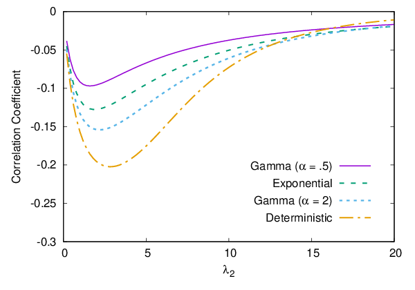
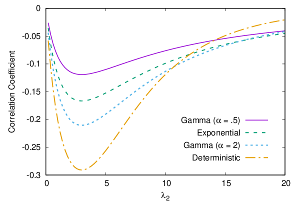
We here confirm the properties of the correlation coefficient of AoIs proved in Proposition 3 through numerical experiments. Throughout the experiments, we use the two-source M/G/1/1 pushout server with a common service time distribution. Figure 1 plots the values of the correlation coefficient for different values of $\lambda_{2}$ when the values of $\lambda_{1}$ and $\mathbb{E}_{\Phi}^{0}[S_{0}]$ are fixed, where Figure 1a) and 1b) show the cases of $(\lambda_{1},1/\mathbb{E}_{\Phi}^{0}[S_{0}])=(1.0,6.0)$ and $(\lambda_{1},1/\mathbb{E}_{\Phi}^{0}[S_{0}])=(3.0,6.0)$ , respectively. Note that $1/\mathbb{E}_{\Phi}^{0}[S_{0}]=\mu/\alpha$ when the service times are gamma distributed with shape parameter $\alpha>0$ and rate parameter $\mu>0$ . From these figures, we can see property 1) in Proposition 3; that is, the correlation coefficient goes to zero as $\lambda_{2}\downarrow 0$ and as $\lambda_{2}\to\infty$ . As another property, we remark that the correlation coefficient takes the minimum value at $\lambda_{2}=1/\mathbb{E}_{\Phi}^{0}[S_{0}]-\lambda_{1}$ in the case of Figure 1b), but it does not in the case of 1a). It does not contradict properties 2) and 4) in Proposition 3; that is, when $\lambda_{1}$ and $\lambda_{2}$ are given, the correlation coefficient takes the minimum value when $1/\mathbb{E}_{\Phi}^{0}[S_{0}]=\lambda=\lambda_{1}+\lambda_{2}$ , but when $\lambda_{1}$ and $\mathbb{E}_{\Phi}^{0}[S_{0}]$ are given, it does not always take the minimum value at either $\lambda_{2}=1/\mathbb{E}_{\Phi}^{0}[S_{0}]-\lambda_{1}$ or $\lambda_{2}=\lambda_{1}$ .

Refer to caption — (a) $\lambda_{1}=1.0$ , $1/\mathbb{E}_{\Phi}^{0}[S_{0}]=6.0$

Figure 2 plots the values of the correlation coefficient of AoIs for different values of $1/\mathbb{E}_{\Phi}^{0}[S_{0}]$ when $\lambda_{1}$ and $\lambda_{2}$ are fixed. Figure 2a) and 2b) show respectively the cases of $\lambda_{1}=\lambda_{2}$ and $\lambda_{1}\neq\lambda_{2}$ while the value of $\lambda=\lambda_{1}+\lambda_{2}$ remains the same in both the figures. From these figures, we can observe the properties 2), 3) and 4) in Proposition 3; that is, the correlation coefficient goes to zero as $1/\mathbb{E}_{\Phi}^{0}[S_{0}]\downarrow 0$ and as $1/\mathbb{E}_{\Phi}^{0}[S_{0}]\to\infty$ ; when $\lambda=\lambda_{1}+\lambda_{2}$ is fixed, the correlation coefficient takes the minimum value when the service times are deterministic and equal to $\lambda^{-1}$ , in addition, when the service times are gamma distributed, it takes the minimum value when $1/\mathbb{E}_{\Phi}^{0}[S_{0}]=\lambda$ , where these minimum values are further minimized when $\lambda_{1}=\lambda_{2}=\lambda/2$ .

V Conclusion

In this paper, we have considered multi-source status update systems and have provided a framework to investigate the joint performance of multiple AoIs, which are defined for the individual sources. Specifically, we have derived a general formula satisfied by the joint Laplace transform of the stationary AoIs. Then, we have applied this formula to a multi-source pushout server and have shown a closed-form formula of the joint Laplace transform of the AoIs in the case with independent M/G inputs. Furthermore, we have revealed some properties of the correlation coefficient of AoIs in the two-source system. In the future, we expect that our general formula will be utilized to evaluate the joint performance of AoIs in many multi-source status update systems and will become useful for development of various systems in the real world.

Appendix A Proof of Lemma 1

We suppose that all random elements in this paper is defined on a probability space $(\Omega,\mathcal{F},\mathbb{P})$ . A family of shift operators $\{\theta_{t}\}_{t\in\mathbb{R}}$ is defined on $(\Omega,\mathcal{F})$ such that $\theta_{t}$ : $\Omega\to\Omega$ is measurable and bijective satisfying $\theta_{s}\circ\theta_{t}=\theta_{s+t}$ for $s$ , $t\in\mathbb{R}$ , where $\theta_{0}$ is the identity; so that $\theta_{t}^{-1}=\theta_{-t}$ for $t\in\mathbb{R}$ . The probability measure $\mathbb{P}$ is assumed to be invariant to $\{\theta_{t}\}_{t\in\mathbb{R}}$ (in other words, $\{\theta_{t}\}_{t\in\mathbb{R}}$ preserves $\mathbb{P}$ ) in the sense that $\mathbb{P}\circ\theta_{t}^{-1}=\mathbb{P}$ for $t\in\mathbb{R}$ . Then, we can assume that the marked point process $\Psi_{C,D}$ satisfying Assumption 1 is compatible with $\{\theta_{t}\}_{t\in\mathbb{R}}$ in the sense that $(U_{n},C_{n},D_{n})\circ\theta_{t}=(U_{\Psi(0,\,t]+n}-t,C_{\Psi(0,\,t]+n},D_{\Psi(0,\,t]+n})$ for each $n\in\mathbb{Z}$ and $t\in\mathbb{R}$ , where $\Psi(0,\,t]=-\Psi(t,\,0]$ for $t<0$ conventionally (see [19]).

In the setup above, the proof of the first assertion in Lemma 1 is achieved by showing that, for each $k\in\mathcal{K}$ , the marked point process $\Psi_{k,D}$ and the AoI process $\{A_{k}(t)\}_{t\in\mathbb{R}}$ are both compatible with $\{\theta_{t}\}_{t\in\mathbb{R}}$ . We first confirm $\Psi_{k,D}$ . By (1), $\Psi_{k,D}$ satisfies

	$\displaystyle\Psi_{k,D}(B\times E)$	$\displaystyle=\sum_{n\in\mathbb{Z}}\bm{1}_{B}(U_{k,n})\,\bm{1}_{E}(D_{k,n}).$
		$\displaystyle=\sum_{n\in\mathbb{Z}}\bm{1}_{B}(U_{n})\,\bm{1}_{E}(D_{n})\,\bm{1}_{\{k\}}(C_{n}),\quad B\in\mathcal{B}(\mathbb{R}),\>E\in\mathcal{B}([0,\infty)).$

The compatibility of $\Psi_{C,D}$ with $\{\theta_{t}\}_{t\in\mathbb{R}}$ implies that, for each $n\in\mathbb{Z}$ and $t\in\mathbb{R}$ , there exists a unique $n^{\prime}\in\mathbb{Z}$ such that $(U_{n}-t,C_{n},D_{n})=(U_{n^{\prime}},C_{n^{\prime}},D_{n^{\prime}})\circ\theta_{t}$ and then

	$\displaystyle\Psi_{k,D}((B+t)\times E)$	$\displaystyle=\sum_{n\in\mathbb{Z}}\bm{1}_{B+t}(U_{n})\,\bm{1}_{E}(D_{n})\,\bm{1}_{\{k\}}(C_{n})$
		$\displaystyle=\sum_{n^{\prime}\in\mathbb{Z}}\bigl(\bm{1}_{B}(U_{n^{\prime}})\,\bm{1}_{E}(D_{n^{\prime}})\,\bm{1}_{\{k\}}(C_{n^{\prime}})\bigr)\circ\theta_{t}$
		$\displaystyle=\Psi_{k,D}(B\times E)\circ\theta_{t},$

where $B+t=\{s+t\mid s\in B\}$ for $t\in\mathbb{R}$ and $B\in\mathcal{B}(\mathbb{R})$ ; that is, $\Psi_{k,D}$ is compatible with $\{\theta_{t}\}_{t\in\mathbb{R}}$ . Therefore, we can show from (2) that $A_{k}(s+t)=A_{k}(s)\circ\theta_{t}$ for any $s$ , $t\in\mathbb{R}$ in a similar way; that is, $\{A_{k}(t)\}_{t\in\mathbb{R}}$ is also compatible with $\{\theta_{t}\}_{t\in\mathbb{R}}$ .

We next show the second assertion in Lemma 1. Since the events $\{D_{k,0}<\infty\}$ and $\{U_{k,1}-U_{k,0}<\infty\}$ are $\mathbb{P}_{\Psi_{k}}^{0}$ -a.s. and $\{\theta_{U_{k,n}}\}_{n\in\mathbb{Z}}$ -invariant under Assumption 1, (2) ensures that the event $\{A_{k}(0)<\infty\}$ is $\mathbb{P}_{\Psi_{k}}^{0}$ -a.s. and $\{\theta_{U_{k,n}}\}_{n\in\mathbb{Z}}$ -invariant as well. Hence, [19, p. 51, Property 1.6.2] says that $A_{k}(0)<\infty$ $\mathbb{P}$ -a.s.

Appendix B Proof of Lemma 2

First, the simplicity of $\Psi$ is inherited from $\Phi$ . We next check 1-2). In the same setting as in Section A, we can assume that the marked point process $\Phi_{c,S}$ satisfying Assumption 2 is compatible with $\{\theta_{t}\}_{t\in\mathbb{R}}$ in the sense that $(T_{n},c_{n},S_{n})\circ\theta_{t}=(T_{\Phi(0,\,t]+n}-t,c_{\Phi(0,\,t]+n},S_{\Phi(0,\,t]+n})$ for each $n\in\mathbb{Z}$ and $t\in\mathbb{R}$ , where $\Phi(0,t]=-\Phi(t,0]$ for $t<0$ . Then, we can see from (12) that $\Psi_{C,D}((B+t)\times\{k\}\times E)=\Psi_{C,D}(B\times\{k\}\times E)\circ\theta_{t}$ holds for any $t\in\mathbb{R}$ , $k\in\mathcal{K}$ , $B\in\mathcal{B}(\mathbb{R})$ and $E\in\mathcal{B}([0,\infty))$ ; that is, $\Psi_{C,D}$ is also compatible with $\{\theta_{t}\}_{t\in\mathbb{R}}$ .

We now confirm 1-3) with (13). Let $\chi(t)$ denote the indicator that $\chi(t)=1$ when the server is occupied by a packet at time $t$ and $\chi(t)=0$ otherwise. Then, $\chi(t)$ satisfies

\chi(t)=\sum_{n\in\mathbb{Z}}\bm{1}_{[T_{n},\,T_{n}+\tau_{n}\wedge S_{n})}(t),\quad t\in\mathbb{R},

which shows that $\{\chi(t)\}_{t\in}$ is also jointly stationary with $\Phi_{c,S}$ . Furthermore, $\{\chi(t)\}_{t\in\mathbb{R}}$ satisfies

\chi(1)=\chi(0)+\Phi(0,1]-\Psi(0,1]-\sum_{n\in\mathbb{Z}}\bm{1}_{(0,1]}(T_{n})\,\bm{1}_{\{S_{n-1}>\tau_{n-1}\}},

where the last term on the right-hand side represents the number of pushouts during $(0,1]$ . Taking the expectations on both the sides above, the stationarity of $\{\chi(t)\}_{t\in\mathbb{R}}$ implies

	$\displaystyle\lambda_{\Psi}$	$\displaystyle=\lambda-\mathbb{E}\biggl[\sum_{n\in\mathbb{Z}}\bm{1}_{(0,1]}(T_{n})\,\bm{1}_{\{S_{n-1}>\tau_{n-1}\}}\biggr]$
		$\displaystyle=\lambda-\lambda\,\mathbb{P}_{\Phi}^{0}(S_{0}>\tau_{0})=\lambda\,\mathbb{P}_{\Phi}^{0}(S_{0}\leq\tau_{0}),$		(36)

and (13) holds.

For 1-4) with (14), the Neveu’s exchange formula (see [19, p. 21]) shows that

	$\displaystyle\lambda_{\Psi}\,\mathbb{P}_{\Psi}^{0}(C_{0}=k)$	$\displaystyle=\lambda\,\mathbb{E}_{\Phi}^{0}\biggl[\sum_{n\in\mathbb{Z}}\bm{1}_{\{C_{n}=k\}}\bm{1}_{[0,\,T_{1})}(U_{n})\biggr]$
		$\displaystyle=\lambda\,\mathbb{P}_{\Phi}^{0}(c_{0}=k,\,S_{0}\leq\tau_{0}),$		(37)

where the second equality follows from the observation that there exists at most one service completion during $[0,\,T_{1})$ and it occurs only when the packet generated at $0$ is completed for service without interruption. Equation (14) then follows from (B) and (B).

Finally, 1-5) is immediate from Neveu’s exchange formula as

\displaystyle\lambda_{\Psi_{k}}\,\mathbb{P}_{\Psi_{k}}^{0}(D_{0}<\infty)

\displaystyle=\lambda_{k}\,\mathbb{E}_{\Phi_{k}}^{0}\biggl[\sum_{n\in\mathbb{Z}}\bm{1}_{\{D_{n}<\infty\}}\,\bm{1}_{[0,T_{k,1})}(U_{k,n})\biggr]=\lambda_{k}\,\mathbb{P}_{\Phi_{k}}^{0}(S_{0}\leq\tau_{0}),

where $\{T_{k,n}\}_{n\in\mathbb{Z}}$ denotes the sub-sequence of $\{T_{n}\}_{n\in\mathbb{Z}}$ corresponding to $\Phi_{k}$ satisfying $\cdots<T_{k,0}\leq 0<T_{k,1}<\cdots$ and the second equality follows from a similar observation to (B). Hence, 1-5) holds since the equality $\lambda_{\Psi_{k}}=\lambda_{\Psi}\,\mathbb{P}_{\Psi}^{0}(C_{0}=k)=\lambda_{k}\,\mathbb{P}_{\Phi_{k}}^{0}(S_{0}\leq\tau_{0})$ is obtained by (13) and (14).

References

[1] Y. Jiang, K. Tokuyama, Y. Wada, and M. Yajima, “Correlation coefficient analysis of the age of information in multi-source systems,” 2020, submitted for presentation at a conference.
[2] S. Kaul, M. Gruteser, V. Rai, and J. Kenney, “Minimizing age of information in vehicular networks,” in 2011 8th Annual IEEE Communications Society Conference on Sensor, Mesh and Ad Hoc Communications and Networks (SECON 2011), 2011, pp. 350–358.
[3] S. Kaul, R. Yates, and M. Gruteser, “Real-time status: How often should one update?” in 2012 Proceedings IEEE INFOCOM, 2012, pp. 2731–2735.
[4] A. Kosta, N. Pappas, and V. Angelakis, “Age of information: A new concept, metric, and tool,” Foundations and Trends in Networking, vol. 12, pp. 162–259, 2017.
[5] Y. Sun, I. Kadota, R. Talak, E. Modiano, and R. Srikant, Age of Information: A New Metric for Information Freshness. Morgan & Claypool, 2019.
[6] S. K. Kaul, R. D. Yates, and M. Gruteser, “Status updates through queues,” in 2012 46th Annual Conference on Information Sciences and Systems (CISS 2012), 2012.
[7] R. D. Yates and S. K. Kaul, “Real-time status updating: multiple sources,” in 2012 IEEE International Symposium on Information Theory Proceedings (ISIT 2012), 2012, pp. 2666–2670.
[8] ——, “The age of information: Real-time status updating by multiple sources,” IEEE Transactions on Information Theory, vol. 65, pp. 1807–1827, 2019.
[9] M. Costa, M. Codreanu, and A. Ephremides, “Age of information with packet management,” in 2014 IEEE International Symposium on Information Theory Proceedings (ISIT 2014), 2014, pp. 1583–1587.
[10] ——, “On the age of information in status update systems with packet management,” IEEE Transactions on Information Theory, vol. 62, pp. 1897–1910, 2016.
[11] A. Kosta, N. Pappas, A. Ephremides, and V. Angelakis, “Age and value of information: Non-linear age case,” in 2017 IEEE International symposium on Information Theory (ISIT 2017), 2017, pp. 326–330.
[12] ——, “The cost of delay in status updates and their value: Non-linear ageing,” IEEE Transactions on Communications, 2020, Early Access.
[13] E. Najm and R. Nasser, “Age of information: The gamma awakening,” in 2016 IEEE International symposium on Information Theory (ISIT 2016), 2016, pp. 2574–2578.
[14] L. Huang and E. Modiano, “Optimizing age-of-information in a multi-class queueing system,” in 2015 IEEE International symposium on Information Theory (ISIT 2015), 2015, pp. 1681–1685.
[15] E. Najm and E. Telatar, “Status updates in a multi-stream M/G/1/1 preemptive queue,” in IEEE Conference on Computer Communications (INFOCOM 2018) Workshops, 2018, pp. 124–129.
[16] Y. Inoue, H. Masuyama, T. Takine, and T. Tanaka, “The stationary distribution of the age of information in FCFS single-server queues,” in 2017 IEEE International symposium on Information Theory (ISIT 2017), 2017, pp. 571–575.
[17] ——, “A general formula for the stationary distribution of the age of information and its application to single-server queues,” IEEE Transactions on Information Theory, vol. 65, pp. 8305–8324, 2019.
[18] G. Kesidis, T. Konstantopoulos, and M. Zazanis, “The distribution of age-of-information performance measures for message processing systems,” 2019, arXiv:1904.05924 [cs.PF].
[19] F. Baccelli and P. Brémaud, Elements of Queueing Theory: Palm Martingale Calculus and Stochastic Recurrences, 2nd ed. Springer, 2003.
[20] G. Last and M. Penrose, Lectures on the Poisson Process. Cambridge University Press, 2017.
[21] F. Baccelli, B. Błaszczyszyn, and M. Karray, “Random measures, point processes, and stochastic geometry,” 2020, https://hal.inria.fr/hal-02460214.