The case for decaying spin-3/2 dark matterPreprint: UMN–TH–3919/20, FTPI–MINN–20/18Preprint: IFT-UAM/CSIC-20-84
Abstract
We consider a spin- particle and show that with a Planck reduced coupling, we can obtain a sufficiently long lifetime making the spin- particle a good dark matter candidate. We show that this dark matter candidate can be produced during inflationary reheating through the scattering of Standard Model particles. The relic abundance as determined by Planck and other experimental measurements is attained for reasonable values of the reheating temperature GeV. We consider two possible gauge invariant couplings to the extended Standard Model. We find a large range of masses are possible which respect the experimental limits on its decay rate. We expect smoking-gun signals in the form of a monochromatic photon with a possible monochromatic neutrino, which can be probed in the near future in IceCube and other indirect detection experiments.
I Introduction
Almost 90 years ago, in 1933, F. Zwicky published a work that shed the first light on the presence of dark matter in the Coma cluster Zwicky:1933gu, confirmed by Babcock in his Ph.D. thesis while measuring the rotation curves of Andromeda babcock. Several studies, including the study of the stability of large-scale structures Ostriker:1973uit confirmed the hypothesis of a dark component in the Universe. Dark matter composed of a new weakly interacting massive neutral particle (WIMP) was proposed by Steigman et al. Gunn:1978gr in 1978, and its precise abundance determination was made from cosmic microwave background measurements by the Planck satellite planck and other experiments. Despite being attractive, the WIMP paradigm is in tension with direct detection measurements (see Arcadi:2017kky for a review). Indeed, the limit on the WIMP-nucleon scattering cross section is for GeV XENON; LUX; PANDAX. The next generation of experiments will probe cross sections as low as Aalbers:2016jon, approaching the irreducible neutrino background nuback, which correspond to a Beyond the Standard Model (BSM) scale of roughly 1 PeV, i.e. significantly above the electroweak scale. The WIMP paradigm is based on the supposition that the dark matter was initially in thermal equilibrium with the Standard Model (SM) sector before decoupling (freeze-out). As such, its lack of dependence on initial conditions remains attractive. However, its lack of discovery to date may be implying that out-of-equilibrium processes dominate the production of dark matter. The freeze-in paradigm fimp; Bernal:2017kxu is an interesting alternative.
The main idea behind freeze-in is that the dark sector is highly secluded from the visible sector. This seclusion may be due to a coupling so small so as to prevent the dark matter from equilibrating with the SM thermal bath. Unlike a WIMP and thermal freeze-out, any dark matter produced this way will have its abundance frozen in. An early example of a such a candidate is the gravitino gravitino, produced through thermal scattering during reheating bbb; Moroi:1995fs; Ellis:2015jpg, yet never achieving equilibrium. There are of course many other options which include the existence of a very heavy mediator, above the maximum temperature reached during reheating, but below the Planck scale, which also prevents the dark sector from coming into thermal equilibrium with the primordial plasma.
This framework is quite common in SO(10)-like models Mambrini:2013iaa; MO, high-scale supersymmetry (SUSY) Benakli:2017whb; grav2; grav3, moduli portals Chowdhury:2018tzw, spin-2 portals Bernal:2018qlk, portals Bhattacharyya:2018evo or other types of heavy mediators HighlyDecoupled. Depending on the specific model, the production rate may be sensitive to the details of reheating, and in particular, to the effects of non-instantaneous reheating Giudice:2000ex; Ellis:2015jpg; Garcia:2017tuj; Garcia:2020eof; Bernal:2020bfj; Bernal:2020gzm, thermalization Garcia:2018wtq, contributions from inflaton decay Kaneta:2019zgw or the details of the inflaton potential leading to reheating Bernal:2019mhf; Garcia:2020eof; bernal.
Of course, the specific identity of the dark matter candidate can significantly affect its production rate. Nature has provided us with a spin-0 particle, spin- matter fields, spin-1 gauge fields, and a spin-2 graviton. Is a spin- dark matter particle the missing piece in the puzzle? Of course, the gravitino appears naturally in local supersymmetry, or supergravity, and as remarked above, was even one of the first dark matter candidates ever proposed. However, when Rarita and Schwinger in 1941 Rarita:1941mf decided to simplify the (overly general) Fierz-Pauli framework Fierz:1939ix, proposing a Lagrangian for a free spin- field, they were obviously not motivated by any arguments based on supersymmetry.
It is well known that a massive spin- particle directly coupled to a gauge field could potentially generate some acausal pathologies velo if not treated correctly in a coherent UV framework. This is in fact the case for any model including particles with spin . For example in extended gauged supergravity, the superluminal propagation of the graviphoton is cured by gravitational backreaction. It is also possible to consider a non-minimal Rarita-Schwinger Lagrangian Porrati:2009bs, by adding non-minimal gauge invariant terms in the action. In any case, we do not consider a spin- particle which is charged under a symmetry and the potential issues raised in velo do not apply to our work.
There have been several studies of spin- WIMP-like dark matter candidates. Effective operators coupling spin- dark matter to the Standard Model were considered for annihilations (in a freeze-out scenario and indirect detection) and scatterings (for direct detection) in Yu:2011by. Effective interactions for spin- dark matter were also considered in eff. Spin- dark matter has been recently explored in Chang:2017dvm where they proposed a WIMP-like candidate in a Higgs-portal scenario. The detection rate in colliders was considered in Christensen:2013aua. For other recent work see Savvidy:2012qa. In every case, the spin- dark matter is protected by a symmetry to stabilize it as it is otherwise assumed to have weak scale interactions.
In our work, we propose an extremely simple and minimal setup, where the SM model is extended with a right-handed neutrino sector needed for the seesaw mechanism for neutrino masses seesaw. The spin- dark matter is coupled to a single fermion and gauge field strength. The fermion is a SM singlet right-handed neutrino, and therefore, the only SM choice for the gauge field is the hypercharge gauge boson . This is necessarily a dimension-5 operator and is suppressed by a BSM scale which permits a long lifetime while at the same time serves as a portal to the SM through the left-right mixing in the neutrino sector. We also include an explicit lepton number violating dimension-5 operator coupling the spin- to the SM Higgs and lepton doublets as allowed by gauge invariance. We consider each of these couplings separately. We show that for a large part of the parameter space, it is possible to satisfy the lifetime constraints and obtain a sufficient (and not excessive) relic density through production during reheating.
The paper is organized as follows. We introduce the model in Sec. II. The Lagrangian of interest will include the aforementioned dimension-5 operators and the neutrino sector giving rise to the seesaw mechanism seesaw. In Sec. III, we consider first the dark matter lifetime. Assuming that the dark matter mass, , is less than the mass of the right-handed neutrino, , the dark matter can decay into a light neutrino and gauge boson. We then consider the production of dark matter through scattering during reheating and directly from inflaton decay. The allowed parameter space of the model is examined in Sec. IV, and we consider the observational signatures of the model in Sec. V. We summarize in Sec. VI.
II The model
II.1 Motivations
A massive spin- particle is described by the Rarita-Schwinger Lagrangian11 1 Our metric convention is . In Appendix A, we provide a simple derivation of the Rarita-Schwinger Lagrangian. Rarita:1941mf
| (1) |
where and . One can extract the equations of motion describing a spin- particle
| (2) |
along with an extra condition appropriate for a spin-1 field
| (3) |
which can be deduced from the preceding constraints. We emphasize that the condition severely limits the operators available to couple a spin- field to the Standard Model sector as we discuss below.
II.2 The Lagrangian
In any UV completion of the SM which contains local supersymmetry, there is at least one spin- particle, the gravitino, with well-defined couplings to SM fields. These are governed by gauge invariance and perhaps other symmetries, such as -parity, that the full theory contains. In a non-supersymmetric theory, or in a theory with high-scale supersymmetry Benakli:2017whb; grav2; grav3 at mass scales below that of the superpartners, the couplings of any spin- field become greatly limited.
Here, we do not consider a specific UV theory which contains the spin- field, and therefore we use gauge invariance to define any possible coupling to the SM which includes a right-handed and/or sterile neutrino sector. Our beyond the SM Lagrangian can be defined by
| (4) |
where and are defined below.
The most general Lagrangian coupling of a spin- field to the SM including a right-handed and/or sterile neutrino, , consistent with Lorentz and gauge invariance is
| (5) | |||||
It is straightforward to show that dimension-4 operators of the type or dimension-5 operators are the only other Lorentz and gauge invariant operators and vanish due to the constraint given in Eq. (2). In Eq. (5), is the field strength of the Standard Model hypercharge gauge boson, , is the SM Higgs doublet and a SM lepton doublet. Due to the unknown and surely model-dependent origin of the spin- field, we have scaled its couplings in by (where GeV is the reduced Planck mass), and therefore we can allow the couplings, , to take values larger as well as smaller than 1.
Both couplings in Eq. (5) are gauge and Lorentz invariant, and can be seen as low energy couplings for gravitino dark matter in high-scale SUSY constructions.22 2 We will not develop this analogy any further as we prefer to remain as general as possible. We note for example, in the SSM the right-handed neutrino can mix with the Bino and generate the coupling Choi:2009ng and an -parity violating coupling of the type would generate the coupling. It is important to note that if a model contains a SM singlet such as a right-handed (or sterile) neutrino, in the absence of symmetry which prevents it, the coupling scaled by is present. In supersymmetric models, -parity would prevent both couplings in Eq. (5). If -parity is broken, signatures of gravitino dark matter are typically a final state, as will be the case here.
In addition, we include a contribution to the Lagrangian which can accommodate the seesaw mechanism seesaw for neutrino masses when right-handed neutrinos are included. This part of the Lagrangian is commonly written as
| (6) |
where the first term provides a Dirac mass when the SM Higgs picks up a vacuum expectation value, and the second term provides a Majorana mass, for the right-handed neutrino. Even if , a coupling of the type in Eq. (6) will generate three- and/or four-body decays of . As a consequence, spin- dark matter is naturally unstable. We will refer to our metastable candidate as the raritron, an obvious tribute to the Rarita-Schwinger field.33 3 It is interesting to note that the article immediately following the original work of Rarita-Schwinger Rarita:1941mf, computed the -decay spectrum of a spin- neutrino Kusaka. This followed Oppenheimer’s suggestion opp that the neutrino may have a spin other than .
The Yukawa term generates mixing between the neutral () and the charged () neutrino sectors, and one can define the mass eigenstates
| (7) | |||
| (8) |
with
| (9) |
where we have assumed (which corresponds to a classical seesaw mechanism of type I) and GeV is the vacuum expectation value of the Standard Model Higgs boson. We have considered for simplicity only one active neutrino generation, and the extension to three families is straightforward. represents the mixing between the two sectors, and is expected to be small for large values of , consistent with recent limits on ( eV sumnu).
III The constraints
The Lagrangian we consider contains two gauge invariant operators with couplings and . In general, the contribution to the raritron decay rate is dominated by the term proportional to as there is no suppression from the heavy right-handed neutrino mass. However, we examine the consequences of each of these terms separately. We begin with the case where is sufficiently small that it can be neglected. In the subsequent subsection, we consider the case where the rates are dominated by and neglect the contributions from .
III.1 Constraints from
III.1.1 The lifetime ()
Depending on its mass, the dominant decay channel for the raritron, , may contain either two or three final states. The two-body decay channel is always available. For , the final state is open and the two-body final state dominates for TeV. When , the channel opens up as seen in Fig. 1. For TeV, the three-body final state dominates the decay width.

The decay rates for the two-body decays and are
| (10) |
where and denotes the Weinberg angle. The processes that produce the antineutrinos have the same decay rate, i.e. and .
In the limit , we find the following total two-body decay width
| (11) |
For the three-body decays and , we find
| (12) | ||||
| (13) |
where the expression for is given in Appendix B. The 3-body decays to antiparticles have the same production rate and .
In the limit , the total three-body decay rate is given by
| (14) |
The total two- and three-body decay rates when correspond to lifetimes
| (15) |
Note that in contrast to Dudas:2014bca (but like Dudas:2020sbq), the four-body decay will not dominate over the three-body decay for large values of , because of a suppression factor of order between the two modes of decay.
III.1.2 The relic abundance from scattering ()
The raritron can be produced directly from the thermal bath during reheating, which is assumed to be a result of inflaton decay. To compute the dark matter density, , we consider the out-of-equilibrium dark matter annihilation processes, , , and , as depicted in Fig. 2. We can write the Boltzmann equation as
| (16) |
where the Hubble parameter for the radiation-dominated Universe is given by
| (17) |
It is convenient to rewrite the Boltzmann equation (16) as
| (18) |
with .
The dark matter production rate (per unit volume per unit time) is represented by
| (19) |
for the processes , where and correspond to particles in the thermal bath, and correspond to produced particles, and represent the thermal distribution functions of the incoming particles, and is the scattering amplitude for the processes shown in Fig. 2, with the expressions for the scattering amplitudes given in Appendix B. From these, we find the following dark matter production rate,
| (20) |
where is the Riemann zeta function.

It is useful to compare the raritron production rate to that of the gravitino in supersymmetric theories. In weak scale supersymmetry, the dominant production channel is gluon + gluon gravitino + gluino. The dimensionful contributions to the cross section for this process originate from the gravitino vertex , the gluino propagator (), and from phase space, so that the cross section scales as . In this case, the production rate scales as . For the case of raritron production, when , the contribution from the propagator is instead so that the cross section scales as giving a production rate which scales as in Eq. (20).
Since the temperature dependence of the production rate, , has , the final density dark matter density is mostly sensitive to the reheat temperature, , rather than the maximum temperature attained during the reheating process Garcia:2017tuj. Therefore, after integration of Eq. (18), the density at can be written
| (21) |
from which we can calculate the present relic abundance at temperature :
| (22) |
where . In writing Eq. (22), we have substituted Eq. (9) for , assuming a characteristic mass of 0.15 eV for the light neutrino. Note that Eqs. (21) and (22) are derived using an instantaneous reheating approximation. Dropping this approximation results in a density which is about 2 times larger for a production rate proportional to as in Eq. (20) Garcia:2017tuj.
It is interesting to note that the same set of parameters which provide a sufficiently long-lived raritron so as to respect the indirect detection constraints, Eq. (15), also produce a relic density in agreement with Planck data, Eq. (22) for a reasonable reheating temperature GeV.
The scattering processes considered in Fig. 2 led to a scattering cross section that scales with the fourth power of the energy of the scatterers, [c.f. Eq. (85) in Appendix B]. In the classification of Garcia:2017tuj, this corresponds to the scenario (). For such a steep dependence on the energy of the scatterers, the instantaneous thermalization approximation can severely underestimate the magnitude of the relic abundance. Indeed, in Garcia:2018wtq it was found that the production of particles from scatterings in the not-yet-thermalized relativistic plasma, present at the earliest stages of reheating, will generically determine the dark matter abundance if . The decay products have initial momenta , where is the mass of the inflaton, and it is only after interactions in the plasma can equilibrate that . The very energetic particles produced before the thermalization of the Universe can therefore dominate the dark matter density budget despite their dilution by entropy production during the late stages of reheating.
Let us assume for definiteness that the inflaton decays predominantly to Higgs bosons, and subdominantly to neutrinos and gauge bosons. When this is the case, the pre-thermal production rate of raritrons can be easily estimated, following the procedure outlined in Garcia:2018wtq. When reheating ends, the number density of pre-thermally generated raritrons via the processes depicted in Fig. 2 can be written as
| (23) |
where
| (24) |
Here () denotes the branching ratio to light neutrinos (to ), and denotes the gauge coupling strength of the interaction responsible for thermalization during reheating. This results in the following closure fraction,
| (25) |
Note that for the chosen model parameters this non-thermally produced population of raritrons dominates over the thermally produced one (22) if . This “enhancement” of the production rate is dependent on the possibility of producing the parent scatterers , and/or directly from inflaton decay. Substantially suppressing two of these decay channels will lead to a raritron population overwhelmingly dominated by late-time reheating thermal effects, with rate (20). In the following section we specialize to reheating driven by the coupling between the inflaton and . In the case when , the dominant decay channel of is precisely to Higgs bosons, while the decay to neutrinos is suppressed by
| (26) |
which is for the fiducial values considered in (25). Moreover, we assume no direct production of gauge bosons.44 4 The timescale for efficient emission of energetic () gauge bosons from the inflaton decay products is typically larger than the thermalization timescale Harigaya:2014waa; Harigaya:2013vwa; Mukaida:2015ria. This then renders non-thermal production completely negligible in this case. In what follows we will therefore disregard this production mechanism, albeit having in mind that for a different reheating process it could be of importance.
III.1.3 The relic abundance from inflaton decay ()
In principle, it is also necessary to consider dark matter production directly from inflaton decay. We parametrize the total width for inflaton decay as follows,
| (27) |
Inflaton decay produces a thermal bath, and we define the moment of reheating to be the time of inflaton-radiation equality.55 5 We are further assuming a matter-dominated Universe prior to decay and . During the process of reheating, the temperature of the newly created radiation bath falls as , where is the cosmological scale factor. From the solution to the set of Boltzmann/Friedmann equations
| (28) | |||
| (29) | |||
| (30) |
we find Garcia:2020eof
| (31) |
and we can write
| (32) |
The source of the Yukawa coupling is of course model dependent. If the inflaton is directly coupled to the SM, there may be, for example, a direct coupling of the inflaton to the Higgs of the type , or the decay to Standard Model fields may involve loops containing SM and/or BSM fields. As a minimal assumption, we assume first that the inflaton couples directly only to the BSM field through and this is the main source of the reheating.
If , then the decay rate of is simply (), and the raritron is produced through the decay process shown in Fig. 3. The partial width in this case is
| (33) |
where we have assumed that . The branching ratio is therefore given by
| (34) |

For a given branching ratio, the number density of raritrons at the end of reheating will be given by Kaneta:2019zgw; Garcia:2020eof
| (35) |
and the relic density in turn takes the form
| (36) | ||||
| (37) |
As one can see, a very small coupling between the raritron and is required to avoid overclosure.66 6 Since the decay of the inflaton is not instantaneous, entropy production continues for some time beyond inflaton-radiation equality. A numerical calculation shows that this injection of entropy, overlooked in our analytical estimates, reduces the value of by a factor of .
When , the direct decay to is not kinematically allowed. There is a two-body decay and the decay rate for this channel would be given by . However, decay to Higgs and light neutrino pairs can proceed through the loop diagrams shown in Fig. 4 and is computed in Appendix C.77 7 There are also four-body decays with an off-shell , but those rates are highly suppressed, . For , we find the following partial widths to Higgses and neutrinos,
| (38) |
and
| (39) |
where in the decay to , we include the tree-level and one-loop contributions. In this case, the decay to Higgs is clearly dominant and we can associate (38) with a total rate such that .


Inflaton decays to raritrons is also possible when . A tree-level decay to has a rate given by Eq. (33) multiplied by . There is also the loop process shown in Fig. 5 88 8 We note that if there is no direct coupling between the inflaton and (i.e. ), and the inflaton decays directly to SM particles, such as , raritron production through inflaton decay is still possible at two loops. and its partial width is given by 99 9 We find an analogous suppression for the four-body decay to B and 3/2.
| (40) |
where . The loop decay dominates whenever
| (41) |
When , the right-hand side of Eq. (41) should be multiplied by . When the loop dominates, the branching ratio is given by
| (42) |
Using Eq. (36) we can immediately deduce the relic abundance,
| (43) |
In this case too, a small coupling between the raritron and is required to avoid overclosure, though for , it is more easily mitigated by taking a large raritron mass as . As one can see, for a given set of parameters (, , ), the possibility of the direct production of raritrons from inflaton decay opens up a new window, allowing for the production of super-heavy spin-3/2 dark matter. Indeed the raritron mass may be well above the reheating temperature, and then only accessible through decay rather than from scattering.
Larger values of are possible if there are inflaton decay channels directly to the SM. Thus if (defined in Eq. (27)) is much larger than . In this case,
| (44) |
which gives
| (45) | ||||
where we have used (32) to substitute for . Even in this case, we require the product of couplings to obtain the correct relic density.
III.2 Constraints from
Having established the decay and production rates for the raritron stemming from the coupling to the right-handed neutrino sector, we now repeat the analysis when the contributions proportional to are dominant.
III.2.1 The lifetime ()
When the term proportional to dominates raritron decay, two-body decays to , , and are possible provided that .1010 10 For these decay rates, unless otherwise specified, () stands for all of (). The Feynman graphs for these are shown in Fig. 6. When , there are many three-body final states where , and are all produced off shell. These are also shown in Fig. 6

The decay rates for the two-body decays and are
| (46) | ||||
| (47) |
where and . The rate for is twice that of the final state.
In the limit , we find the following total two-body decay width
| (48) |
Comparing Eqs.(11) and (48) we notice that for , this contribution to the two-body decays dominates the raritron lifetime.
For the three-body decay to fermions via Higgs exchange (), we find
| (49) |
where the Yukawa coupling is , is the number of colors of fermion , and the expression for is given in Appendix B. If , we have
| (50) |
which is equal to the product .
For the three-body decay to fermions via -boson exchange (assuming ), we find
| (51) |
where for leptonic decays, and is the Cabibbo-Kobayashi-Maskawa matrix element for decays into quarks. If , we have
| (52) |
equal to .
For the three-body decay to fermions via exchange (), we find
| (53) |
where is given in Appendix B. If , we find
| (54) |
where , denote the axial and vector couplings of . This rate is equal to .
When , we can approximate the total decay rate as
| (55) |
The various two- and three-body partial rates are shown relative to the total two-body rate in Fig. 7.

When , the raritron lifetime is solely determined by the three-body rates, and the number of different fermion final state pairs will depend on the raritron mass. This is clearly seen in Fig. 7 as more partial rates come into play as is increased. Note that for , (and thus ) the three-body decay through Higgs exchange is subdominant. Indeed, we find
| (56) |
The total rate can be expressed by approximate analytic expression in three separate mass regimes. For , the sum of all the three-body final state channels gives a rate slightly larger (by a factor of 1.09) than the two-body rate so that the lifetime for large masses is
| (57) |
For , the two-body rate is kinematically forbidden, and the total three-body rate is complicated by the various thresholds and a single simple expression for the lifetime is not possible. However, for , we can use Eq. (55)
| (58) |
while for we can fit the total three-body rate given by the black line in Fig. 7 and find
| (59) |
As one can see, for the same raritron mass, a sufficiently long lifetime requires as expected. Conversely, for similar values of the couplings, the rate proportional to will produce a long lifetime at small values of the rariton masses. Typically for large enough , we require and only the three-body decay channels are open.
III.2.2 The relic abundance from scattering ()
When is the dominant coupling, there are many channels from which the raritron can be produced directly from the thermal bath during reheating. These include , , , , , as well as many other diagrams mediated by Higgs exchange as depicted in Fig. 8.

The temperature dependence of the production rate rate will depend on the number of raritons in the final state. The total rate is
| (60) | |||||
where the first term corresponds to diagrams with two raritrons in the final state and the second with one. Notice that in both cases the temperature dependence differs from that in processes dominated by discussed in the previous subsection. Indeed, because of the steep temperature dependence for two raritrons in the final state, the relic density from this term will be sensitive to the maximum temperature, attained during reheating, whereas the term stemming from single raritron production will be sensitive only to Garcia:2017tuj.
Following the procedure detailed in Garcia:2017tuj, we obtain the number density of dark matter at , which takes the following form,
| (61) | |||||
where the ratio of to , assuming instantaneous thermalization, is given by Ellis:2015jpg
| (62) |
From this we can calculate the present relic abundance at temperature :
| (63) |
Note that this expression corresponds to that obtained from scatterings with a single raritron in the final state. Indeed, under the constraint that the raritron abundance saturates the observed dark matter relic density, single raritron production dominates over double raritron production for any phenomenologically sensible values of and (see Sec. IV).
When thermalization is not assumed to occur instantaneously, the previous results can be significantly changed, given that the two raritron production cross section scales with the sixth power of the scatterer energy, that is , or in the classification of Garcia:2017tuj. In this case, the number density of non-thermally generated raritrons can be found to be given by
| (64) |
Here
| (65) |
where () denotes the inflaton branching ratio to leptons (to Higgs). The corresponding non-thermal closure fraction can be written as follows,
| (66) |
Comparing this expression with Eq. (63), we obtain that for
| (67) |
it is the non-thermal raritron population that dominates the dark matter energy budget. As in the case of the coupling, in the discussion that follows we will omit this production mechanism due to its dependence on the inflationary model.
In the previous subsection, we considered the production of raritrons from inflaton decay. We assumed that the inflaton was coupled only to the right-handed neutrino. In that case, raritron production from decay is possible only at two loops, and we do not consider that here. In principle one can couple the inflaton directly to the Standard model, but raritron production would be highly model dependent on the inflaton-SM coupling. Therefore in the case of the coupling, we do not consider raritron production from inflaton decay.
IV Results and analysis
IV.1 Results when dominates
In the preceding analysis, we derived the raritron lifetime and density in terms of the Dirac coupling , the right-handed neutrino mass, , and the light neutrino mass, , though these are related through Eq. (9). In addition, there is an absolute theoretical limit on () from perturbativity and an experimental cosmological constraint on the sum of the light neutrino masses which force eV sumnu. In other words, for a given , the upper bound on implies an upper bound on , and as a consequence a lower bound on the raritron lifetime and upper bound on its relic abundance. For example,
| (68) |
We can then express the lifetime constraints (15) as a function of
| (69) |
Given and , limits from the dark matter lifetime (15) give us a lower bound on (we fix eV to be specific). For dark matter production from scattering, we can use the lower bound on to find the reheating temperature necessary to obtain the correct relic abundance in Eq. (22). For dark matter produced from decay, the bound on is not needed. Note that when we saturate the bound on we also have an upper limit on from the perturbativity of , which is GeV.
IV.1.1 Dark matter production from scattering
We consider first the case where dark matter is produced exclusively through scatterings during reheating. That is, we assume that the direct production from inflaton decay is negligible. We show in Fig. 9 the available parameter space in the () plane. In the lower right portion of the plane, the raritron lifetime is too short when compared with experimental constraints. Due to the large range of dark matter masses we apply constraints from several experiments: XMM-Newton observations of M31 Boyarsky:2007ay at the keV scale, SPI, INTEGRAL and COMPTEL observations Boyarsky:2007ge; Yuksel:2007dr at the MeV scale, the latest limits from FERMI-LAT at the GeV scale Ackermann:2015lka, and HESS above the TeV scale Abramowski:2013ax (see also Lattanzi:2013uza). Note that the limits on the dark matter lifetime given by the collaborations correspond to a specific final state. A complete study taking into account the exact shape of the spectrum is beyond the scope of our work, and is not necessary considering the large dependence of the relic abundance on the reheating temperature.

To obtain the limit on the lifetime in the () plane, we first fix the value of at the experimental limit from Eq. (15) for each value of . This determines the combination . Then from Eq. (22), we can determine the value of needed to obtain . This procedure determines the blue line in Fig. 9. For lower masses ( TeV), we use -ray limits, whereas for higher masses ( PeV) we use neutrino limits and the dot-dashed portion of the line in between is an extrapolation. In the shaded region below this line, we continue to fix , but to do so at lower requires lower values of and hence lifetimes below the experimental limit. Conversely, in this shaded region, satisfying the lifetime limit would imply an insufficient relic density (though this cannot be excluded). For reference we also plot in Fig. 9 the line corresponding to a projected sensitivity corresponding to a lifetime of which is similar to the present experimental limits. This line can be determined from the substitution of into giving
| (70) |
resulting in a slope of 4/5 (in the logs) for vs . A change of slope in this line occurs for TeV corresponding to the point when the three-body and two-body decay rates are equal. At higher masses, using we have,
| (71) |
which results in a slope of 6/5.
In the upper left portion of the () plane we fix the value of GeV at its perturbative limit from . In this region, above the blue line, the lifetime is always longer than the experimental limit. Assuming eV, we show three contours with fixed as indicated and . For each value of , the shaded region above the line (at higher ) would have an excessive raritron density. We see immediately that raritron masses from about a keV to a PeV are all allowed for reasonable reheat temperatures GeV.
It is also useful to consider the allowed parameter space in the (, ) plane. We show in Fig. 10 the region allowed for different values of the reheating temperature as indicated. The curves and shadings are as in the previous figure, however, we now fix both eV and GeV everywhere across the plane. In this case, the lifetime limit shown by the blue curve can be viewed as a function of and and should be close to a line with log slope of for low and for larger masses when the three-body decay dominates. As discussed above, we find that values of of order 1 are allowed for relatively low reheating temperatures () whereas higher reheating temperatures of order necessitate to avoid an overabundance of dark matter.

IV.1.2 Including the inflaton decay
Reheating is the result of inflaton decay to SM particles. If , there will be tree-level diagrams which lead to reheating and raritron production. When , there may be a direct coupling between the inflaton and the SM (characterized by the coupling in Eq. (27)) or through loops with as in Fig. 4 and discussed earlier. Even if there is no direct coupling between the inflaton and raritron, raritron production through loops is possible as in Fig. 5. Unless inflaton decay to dark matter is highly suppressed, once a direct decay channel is open even through loops, it can easily dominate the dark matter production Kaneta:2019zgw. We have seen this effect for the specific case of raritron dark matter in the preceding section.
To get an idea of the relevant parameter values, we rewrite Eq. (43) (ignoring the logs) with as
| (72) |
Using this value for in the lifetime in Eq. (15) (using the three-body decay as an example), we find for
| (73) |
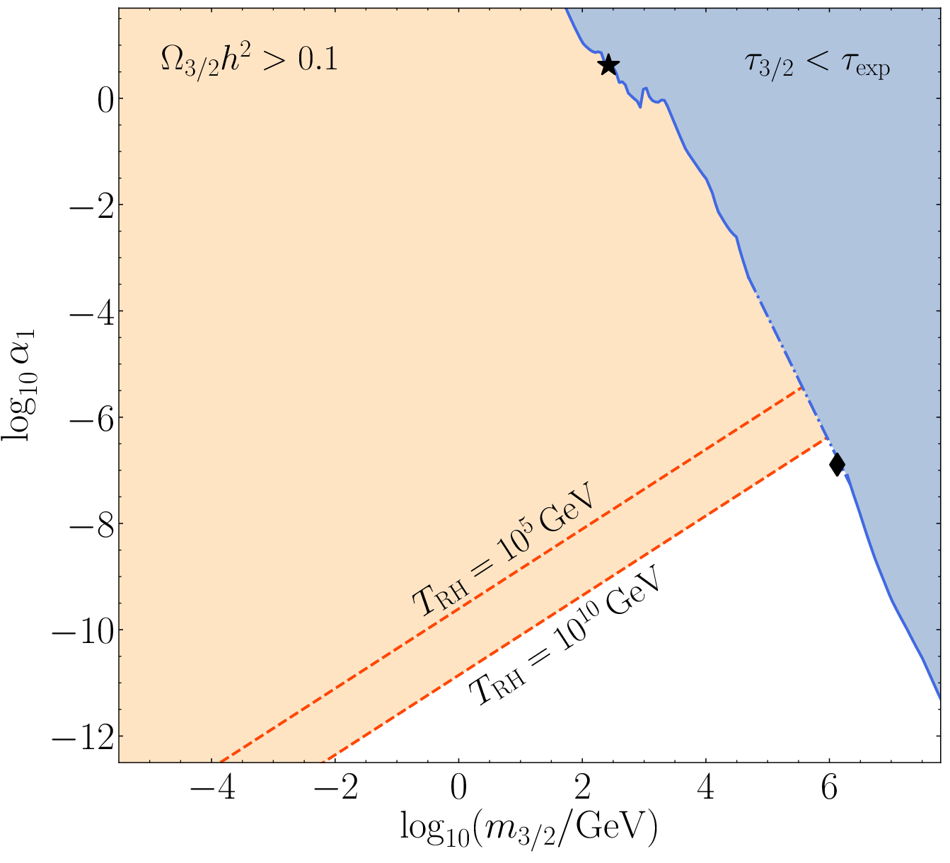
The relevant parameter space in the (, ) plane is shown in Fig. 11. Since the blue line is determined solely from the limit on the raritron lifetime, it is independent of the production mechanism and is the same as in Fig. 10. Comparing Fig. 11 with Fig. 10, we see clearly that the production of dark matter through inflaton decay is much more copious and the parameter space is much more constrained. The relic abundance necessitates much lower values of to avoid overabundance, and the result is much less dependent on as one can see comparing Eqs. (22) and (70), where depends on in the scattering case, compared to the inflaton decay process. This feature is also clearly illustrated in Fig. 11, where we show two lines producing the correct relic abundance with and GeV.
IV.2 Results when dominates
We can now repeat the previous analysis when the raritron is coupled to the SM through . We first show the results in the () plane in Fig. 12 produced in the same manner as in the previous subsection. Due to the model dependence of the abundance of produced raritrons from pre-thermal scatterings, encoded in the effective branching ratio , we limit ourselves here to ratiron production in thermal equilibrium, i.e. Eq. (63). We note that while there is not a direct raritron decay channel with a photon in the final state, photons will be produced. However, in the absence of a simulation of the full decay chain, we show the same experimental limits used in the previous subsection. We also show for reference, the curve corresponding to a lifetime of s. The experimental constraints demanding a sufficiently long lifetime and suitable relic density push the allowed mass range to GeV when GeV, and GeV when GeV. Note that our numerical results include the running of the gauge and Yukawa couplings to the appropriate temperature scale, though not explicitly written in the analytic formulas.

As one can see from comparing Figs. 9 and 12, for a given reheat temperature, and relic density, we need as noted earlier. For example, for MeV, and GeV, we find , whereas, . Similarly, we show the results in the (, ) plane in Fig. 13. We see that unless is very small (), GeV, and the upper limit on the raritron mass decreases with increasing .
We also see by comparing Figs. 10 and 13, that when the reheat temperature is rather large ( GeV), and MeV, the values of needed to produce are similar though quite small. The required difference in the couplings is much greater at smaller .

V Signatures
Having established the viable parameter space for the raritron dark matter model, we now discuss in more detail the possible experimental signatures for such a model. The two-body decay mode shown in Fig. 1 will produce a monochromatic photon and neutrino.1111 11 A signal of this type was termed a “double smoking-gun” in Aisati:2015ova. Spin-3/2 fields were not included in their study, nor in ProfumoPlanck, and they did not try to produce cosmologically viable scenarios. If , there is also a two-body final state . These decay channels are easily observable at detectors and the signal will give us 1) the mass of the dark matter (from the position of the signal in the spectrum) and 2) the lifetime (from the strength of the signal). On top of the monochromatic signal, there will also be a continuous spectrum due to the three-body channels which dominate at higher raritron masses. If the raritron is produced mainly through scattering, the signal can be translated to the reheating temperature needed to obtain the right relic abundance using Eq. (70). For example, a GeV gamma ray observed by FERMI with a signal strength corresponding to a lifetime of s would imply a reheating temperature of GeV. In this case, the temperature is independent of the parameter . In contrast, if the production were dominated by inflaton decays, some information on the combination of and could be ascertained.
As an exercise, we reanalyze one of the most popular recent “signals”: the 130 GeV line observed by the FERMI satellite in 2012 Ackermann:2012qk. This is a monochromatic signal that could be fit with a dark matter mass GeV and a lifetime Kyae:2012vi, for a Navarro, Frenk, and White profile Navarro:1995iw.1212 12 The dependence on the dark matter distribution for decaying dark matter being proportional to its density (versus ) is much weaker than for annihilating dark matter. Interestingly, this kind of signal could correspond to a spin- dark matter decay. For scattering-dominated production, we can use Eq. (70) to determine the reheat temperature, GeV. From the lifetime, we can also determine the combination or upon fixing the light neutrino mass, . We find, GeV-1 or for GeV. Note that for this value of , when inflaton decay is the dominant production mode, the reheating temperature must be extremely (and unphysically) low. Thus not only would we determine the reheat temperature and , but we would also know that inflaton decay does not play a role in dark matter production. This position of this example in the (, ) plane is illustrated in Figs. 10 and 11 by a star. Such a signal, if observed below , could be correlated with a similar monochromatic signal from neutrino detectors like ANTARES or IceCube1313 13 The latter being more sensitive to track events than the ANTARES telescope.. Even if dedicated neutrino line searches have not been yet performed by the IceCube Collaboration, its sensitivity has been calculated in ElAisati:2017ppn and should probe a lifetime of .
Next, we repeat the exercise for the PeV neutrino signal observed by IceCube Aartsen:2014gkd. There were some attempts to explain these events from a dark matter perspective (see Dudas:2014bca for instance) but it was difficult to reconcile the signal with the correct relic abundance. The number of events expected by IceCube is Gandhi:1998ri; Dudas:2014bca
| (74) |
where is defined from the fiducial volume and corresponds to the astrophysical uncertainty in the local distribution of the dark mater halo. The mass and widths are expressed in GeV. A rate of one PeV event per year gives us , corresponding to s.1414 14 This is similar to what was obtained in Feldstein:2013kka, namely, . Using this lifetime, with PeV, we can again determine the value of now from the three-body decay rate which is dominant, . The reheating temperature in this case can be obtained from Eq. (71) and we find GeV, when raritron production is due to scattering. When production is due to inflaton decay, we can use Eq. (73) and find, GeV. The position of this example is displayed in Figs. 10 and 11 by the black diamond. Both the scattering production and the inflaton decay process scenarios are compatible correct relic abundance and the IceCube PeV monochromatic signals.
VI Conclusion
We have shown that a metastable spin- particle can be a suitable dark matter candidate through the introduction of a minimal (Planck-suppressed) coupling, , to a right-handed neutrino. Surprisingly, the parameter space needed to generate a sufficiently long lifetime is perfectly compatible with both the astrophysical constraints from -ray and neutrino experiments as well as the cosmological determination of the dark matter density . Our results are summarized in Figs. 10 and 11 where we display the allowed region in the () plane. We considered both the production of dark matter from the thermal bath produced during reheating, and production directly from inflaton decay. We also have shown that smoking-gun signals are expected from such couplings, in the form of a monochromatic neutrino and/or a monochromatic gamma-ray line.
In addition, we considered a second possible gauge invariant coupling, of the raritron to the SM Higgs and lepton doublet. The requirement of a sufficiently long lifetime and correct relic abundance, restricts the raritron mass range to lower values and lower coupling as seen in Figs. 12 and 13.
We have also illustrated, as examples, the points in the parameter space that could explain the gamma-ray signal observed by the FERMI telescope, or PeV neutrinos observed by IceCube that can be combined with the recent ANITA analysis ANITA. Moreover, it was shown in benakli2 that spin- particles can have an impact on the form of gravitational waves produced during reheating that could be observable in future ultra-high frequency detectors.
Acknowledgments: The authors want to thank especially Kunio Kaneta and Emilian Dudas for very insightful discussions. This work was supported in part by the France-U.S. PICS MicroDark. The work of M.A.G.G. was supported by the Spanish Agencia Estatal de Investigación through the Grants No. FPA2015-65929-P (MINECO/FEDER, UE) and No. PGC2018095161-B-I00, IFT Centro de Excelencia Severo Ochoa Grant No. SEV-2016-0597, and Red Consolider MultiDark Grant No. FPA2017-90566-REDC. This project has received funding/support from the European Union’s Horizon 2020 research and innovation program under the Marie Skodowska-Curie Grant Agreements Elusives ITN No. 674896 and InvisiblesPlus RISE No. 690575. The work of K.A.O. was supported in part by the U.S. DOE Grant No. DE-SC0011842 at the University of Minnesota.
Appendix A The Rarita-Schwinger Lagrangian
Rarita and Schwinger Rarita:1941mf derived the Lagrangian (1) following the work of Fierz and Pauli Fierz:1939ix. One can start with the hypothesis that a spin- particle should respect both the spin- Dirac equation and spin-1 divergence relation, namely,
| (75) | |||
| (76) |
By writing the field in terms of its spin components and after a Clebsch-Gordan decomposition, we have
| (77) |
where is a Dirac spinor of helicity , which is a solution of Eq. (75), and is a vector polarization with spin projection along the direction of the momentum, so that . See Christensen:2013aua for a detailed solution. One can show, using each of the components in Eq. (77) by direct calculation and after a little algebra, that Eqs. (75) and (76) imply
| (78) |
We can construct a Lagrangian for a spin- field, whose Euler-Lagrange equation gives Eq. (75), with terms such as , , or any combinations of that type, which are consistent with the relations (76) and (78). Among the class of possible Lagrangians, the simplest one is
| (79) |
Note that the coefficient of the last four terms in Eq. (79) is arbitrary (e.g., Rarita:1941mf included a factor of 1/3 in front of each of these terms). Equation (79) can be simplified to
| (80) |
which is, up to a normalization factor, our Lagrangian in Eq. (1).
Appendix B Decay and scattering rates
In this appendix, we provide some relevant details concerning the computation of the dark matter decay rate.
B.1 Three-body decay formula
The phase space integration for the three-body decay processes and can be performed analytically if one disregards the small neutrino mass . In this limit, the decay rates are given by Eqs. (12) and (13), where the threshold function is given by the following expression,
| (81) |
where
| (82) |
For the three-body decay processes , we find
| (83) |
and
| (84) |
B.2 Scattering amplitudes
The amplitudes for the scattering processes contributing to dark matter production from the thermal bath, for the case with coupling , can be written as
| (85) | ||||
| (86) | ||||
| (87) |
In the limit of , we find
| (88) | ||||
| (89) | ||||
| (90) |
Similarly, for the interactions mediated by the coupling , assuming , we find
| (91) |
| (92) |
| (93) |
| (94) |
| (95) |
| (96) |
| (97) |
| (98) |
| (99) |
| (100) |
| (101) |
| (102) |
Appendix C Loop Calculations
First, we consider the inflaton decay to two Higgs bosons through the loop process shown in Fig. 4. The amplitude is given by
| (103) |
with the coupling , and the propagators are defined as and , where is the left-handed neutrino mass and is the right-handed neutrino mass. We remind the reader that when , we use the coupling .
To calculate the amplitudes, we use the Passarino-Veltman functions Passarino. The two-point form factors can be expressed as
| (104) |
where
| (105) |
and
| (106) |
and the three-point form factors are given by
| (107) |
where
| (108) |
| (109) |
and
| (110) |
Using the Passarino-Veltman functions, we can express the amplitude (103) as
| (111) |
Assuming we obtain
| (112) |
and the decay rate is given by Eq. (38).
Next, we calculate the inflaton decay rate to left-handed neutrinos through the loop process shown in Fig. 4. The amplitude of this process is
| (113) | ||||
where , , and . Using the Passarino-Veltman functions, we can express the amplitude (113) as
| (114) |
With , , and , we find
| (115) |
and upon substitution of Eq. (9), the decay rate is given by Eq. (39).
Finally, we calculate the inflaton decay rate to raritrons through the loop process shown in Fig. 5. We can express the amplitude as follows,
| (116) |
where , , and . We do not include the full expression of the amplitude (116) in terms of the Passarino-Veltman functions due to its complexity. With , the amplitude takes the form
| (117) |
and the decay rate is given by Eq. (40).
References
- (1) F. Zwicky, “Die Rotverschiebung von extragalaktischen Nebeln,” Helv. Phys. Acta 6 (1933), 110-127
- (2) H. W. Babcock, "The rotation of the Andromeda Nebula". Lick Observatory Bulletin N. 498, Ph.D. thesis, University of California, Berkeley, 1938.
- (3) J. Ostriker and P. Peebles, Astrophys. J. 186 (1973), 467-480
- (4) J. Gunn, B. Lee, I. Lerche, D. Schramm and G. Steigman, Astrophys. J. 223 (1978), 1015-1031
- (5) P. A. R. Ade et al. [Planck Collaboration], Astron. Astrophys. 594, A13 (2016) [arXiv:1502.01589 [astro-ph.CO]]; N. Aghanim et al. [Planck], Astron. Astrophys. 641, A6 (2020) [arXiv:1807.06209 [astro-ph.CO]].
- (6) G. Arcadi, M. Dutra, P. Ghosh, M. Lindner, Y. Mambrini, M. Pierre, S. Profumo and F. S. Queiroz, Eur. Phys. J. C 78 (2018) no.3, 203 [arXiv:1703.07364 [hep-ph]].
- (7) E. Aprile et al. [XENON Collaboration], Phys. Rev. Lett. 121 (2018) no.11, 111302 [arXiv:1805.12562 [astro-ph.CO]].
- (8) D. S. Akerib et al. [LUX Collaboration], Phys. Rev. Lett. 118 (2017) no.2, 021303 [arXiv:1608.07648 [astro-ph.CO]].
- (9) X. Cui et al. [PandaX-II Collaboration], Phys. Rev. Lett. 119 (2017) no.18, 181302 [arXiv:1708.06917 [astro-ph.CO]].
- (10) J. Aalbers et al. [DARWIN], JCAP 11 (2016), 017 [arXiv:1606.07001 [astro-ph.IM]].
- (11) J. Billard, L. Strigari and E. Figueroa-Feliciano, Phys. Rev. D 89 (2014) no.2, 023524 [arXiv:1307.5458 [hep-ph]]; P. Cushman, C. Galbiati, D. N. McKinsey, H. Robertson, T. M. P. Tait, D. Bauer, A. Borgland and B. Cabrera et al., Snowmass Working Group Report: WIMP Dark Matter Direct Detection, arXiv:1310.8327 [hep-ex].
- (12) L. J. Hall, K. Jedamzik, J. March-Russell and S. M. West, JHEP 1003 (2010) 080 [arXiv:0911.1120 [hep-ph]]; X. Chu, T. Hambye and M. H. G. Tytgat, JCAP 1205 (2012) 034 [arXiv:1112.0493 [hep-ph]]; X. Chu, Y. Mambrini, J. Quevillon and B. Zaldivar, JCAP 1401 (2014) 034 [arXiv:1306.4677 [hep-ph]]; A. Biswas, D. Borah and A. Dasgupta, Phys. Rev. D 99, no.1, 015033 (2019) [arXiv:1805.06903 [hep-ph]].
- (13) N. Bernal, M. Heikinheimo, T. Tenkanen, K. Tuominen and V. Vaskonen, Int. J. Mod. Phys. A 32 (2017) no.27, 1730023 [arXiv:1706.07442 [hep-ph]].
- (14) H. Pagels and J. R. Primack, Phys. Rev. Lett. 48, 223 (1982); D. V. Nanopoulos, K. A. Olive and M. Srednicki, Phys. Lett. B 127, 30 (1983); J. Ellis, J. Hagelin, D. Nanopoulos, K. Olive and M. Srednicki, Nucl. Phys. B 238 (1984) 453. M. Y. Khlopov and A. D. Linde, Phys. Lett. B 138, 265 (1984); K. A. Olive, D. N. Schramm and M. Srednicki, Nucl. Phys. B 255, 495 (1985).
- (15) J. R. Ellis, J. E. Kim and D. V. Nanopoulos, Phys. Lett. B 145, 181 (1984); J. R. Ellis, D. V. Nanopoulos, K. A. Olive and S. J. Rey, Astropart. Phys. 4, 371 (1996) [hep-ph/9505438]; G. F. Giudice, A. Riotto and I. Tkachev, JHEP 9911, 036 (1999) [hep-ph/9911302]; M. Bolz, A. Brandenburg and W. Buchmuller, Nucl. Phys. B 606, 518 (2001) [Erratum-ibid. B 790, 336 (2008)] [hep-ph/0012052]; R. H. Cyburt, J. Ellis, B. D. Fields and K. A. Olive, Phys. Rev. D 67, 103521 (2003) [astro-ph/0211258]; F. D. Steffen, JCAP 0609, 001 (2006) [hep-ph/0605306]; J. Pradler and F. D. Steffen, Phys. Rev. D 75, 023509 (2007) [hep-ph/0608344]; V. S. Rychkov and A. Strumia, Phys. Rev. D 75, 075011 (2007) [hep-ph/0701104]; M. Kawasaki, K. Kohri, T Moroi and A.Yotsuyanagi, Phys. Rev. D 78, 065011 (2008) [arXiv:0804.3745 [hep-ph]].
- (16) T. Moroi, hep-ph/9503210.
- (17) J. Ellis, M. A. G. Garcia, D. V. Nanopoulos, K. A. Olive and M. Peloso, JCAP 03 (2016), 008 [arXiv:1512.05701 [astro-ph.CO]].
- (18) Y. Mambrini, K. A. Olive, J. Quevillon and B. Zaldivar, Phys. Rev. Lett. 110 (2013) no.24, 241306 [arXiv:1302.4438 [hep-ph]]; N. Nagata, K. A. Olive and J. Zheng, JHEP 1510, 193 (2015) [arXiv:1509.00809 [hep-ph]]; Y. Mambrini, N. Nagata, K. A. Olive and J. Zheng, Phys. Rev. D 93 (2016) no.11, 111703 [arXiv:1602.05583 [hep-ph]]; X. Chu, Y. Mambrini, J. Quevillon and B. Zaldivar, JCAP 1401 (2014) 034 [arXiv:1306.4677 [hep-ph]]; Y. Mambrini, N. Nagata, K. A. Olive, J. Quevillon and J. Zheng, Phys. Rev. D 91 (2015) no.9, 095010 [arXiv:1502.06929 [hep-ph]]; N. Nagata, K. A. Olive and J. Zheng, JCAP 1702, no. 02, 016 (2017) [arXiv:1611.04693 [hep-ph]].
- (19) R. N. Mohapatra and N. Okada, Phys. Rev. D 101, no.11, 115022 (2020) [arXiv:2005.00365 [hep-ph]].
- (20) K. Benakli, Y. Chen, E. Dudas and Y. Mambrini, Phys. Rev. D 95, no. 9, 095002 (2017) [arXiv:1701.06574 [hep-ph]].
- (21) E. Dudas, Y. Mambrini and K. Olive, Phys. Rev. Lett. 119 (2017) no.5, 051801 [arXiv:1704.03008 [hep-ph]].
- (22) E. Dudas, T. Gherghetta, Y. Mambrini and K. A. Olive, Phys. Rev. D 96 (2017) no.11, 115032 [arXiv:1710.07341 [hep-ph]]; E. Dudas, T. Gherghetta, K. Kaneta, Y. Mambrini and K. A. Olive, Phys. Rev. D 98, no. 1, 015030 (2018) [arXiv:1805.07342 [hep-ph]]. S. A. R. Ellis, T. Gherghetta, K. Kaneta and K. A. Olive, Phys. Rev. D 98, no. 5, 055009 (2018) [arXiv:1807.06488 [hep-ph]].
- (23) D. Chowdhury, E. Dudas, M. Dutra and Y. Mambrini, Phys. Rev. D 99 (2019) no.9, 095028 [arXiv:1811.01947 [hep-ph]].
- (24) N. Bernal, M. Dutra, Y. Mambrini, K. Olive, M. Peloso and M. Pierre, Phys. Rev. D 97 (2018) no.11, 115020 [arXiv:1803.01866 [hep-ph]].
- (25) G. Bhattacharyya, M. Dutra, Y. Mambrini and M. Pierre, Phys. Rev. D 98 (2018) no.3, 035038 [arXiv:1806.00016 [hep-ph]]; A. Banerjee, G. Bhattacharyya, D. Chowdhury and Y. Mambrini, JCAP 12 (2019), 009 [arXiv:1905.11407 [hep-ph]].
- (26) L. Heurtier and F. Huang, Phys. Rev. D 100 (2019) no.4, 043507 [arXiv:1905.05191 [hep-ph]]; A. Berlin, D. Hooper and G. Krnjaic, Phys. Rev. D 94 (2016) no.9, 095019 [arXiv:1609.02555 [hep-ph]]; A. Berlin, D. Hooper and G. Krnjaic, Phys. Lett. B 760 (2016) 106 [arXiv:1602.08490 [hep-ph]]; M. Heikinheimo, T. Tenkanen, K. Tuominen and V. Vaskonen, Phys. Rev. D 94 (2016) no.6, 063506 Erratum: [Phys. Rev. D 96 (2017) no.10, 109902] [arXiv:1604.02401 [astro-ph.CO]].
- (27) G. F. Giudice, E. W. Kolb and A. Riotto, Phys. Rev. D 64 (2001) 023508 [hep-ph/0005123]; D. J. H. Chung, E. W. Kolb and A. Riotto, Phys. Rev. D 60 (1999) 063504 [hep-ph/9809453].
- (28) M. A. G. Garcia, Y. Mambrini, K. A. Olive and M. Peloso, Phys. Rev. D 96 (2017) no.10, 103510 [arXiv:1709.01549 [hep-ph]].
- (29) M. A. G. Garcia, K. Kaneta, Y. Mambrini and K. A. Olive, Phys. Rev. D 101, no.12, 123507 (2020) [arXiv:2004.08404 [hep-ph]].
- (30) N. Bernal, J. Rubio and H. Veermäe, JCAP 06, 047 (2020) [arXiv:2004.13706 [hep-ph]].
- (31) N. Bernal, [arXiv:2005.08988 [hep-ph]].
- (32) M. A. G. Garcia and M. A. Amin, Phys. Rev. D 98, no. 10, 103504 (2018) [arXiv:1806.01865 [hep-ph]].
- (33) K. Kaneta, Y. Mambrini and K. A. Olive, Phys. Rev. D 99 (2019) no.6, 063508 [arXiv:1901.04449 [hep-ph]].
- (34) N. Bernal, F. Elahi, C. Maldonado and J. Unwin, JCAP 11, 026 (2019) [arXiv:1909.07992 [hep-ph]]; P. Arias, N. Bernal, A. Herrera and C. Maldonado, JCAP 10 (2019), 047 [arXiv:1906.04183 [hep-ph]].
- (35) N. Bernal, J. Rubio and H. Veermäe, [arXiv:2006.02442 [hep-ph]].
- (36) W. Rarita and J. Schwinger, Phys. Rev. 60 (1941), 61
- (37) M. Fierz and W. Pauli, Proc. Roy. Soc. Lond. A A173 (1939), 211-232 doi:10.1098/rspa.1939.0140
- (38) G. Velo and D. Zwanziger, Phys. Rev. 188, 2218-2222 (1969); G. Velo and D. Zwanziger, Phys. Rev. 186, 1337-1341 (1969).
- (39) M. Porrati and R. Rahman, Phys. Rev. D 80, 025009 (2009) [arXiv:0906.1432 [hep-th]].
- (40) Z. H. Yu, J. M. Zheng, X. J. Bi, Z. Li, D. X. Yao and H. H. Zhang, Nucl. Phys. B 860 (2012), 115-151 [arXiv:1112.6052 [hep-ph]].
- (41) R. Ding and Y. Liao, JHEP 04, 054 (2012) [arXiv:1201.0506 [hep-ph]]; R. Ding, Y. Liao, J. Y. Liu and K. Wang, JCAP 05, 028 (2013) [arXiv:1302.4034 [hep-ph]].
- (42) C. F. Chang, X. G. He and J. Tandean, Phys. Rev. D 96 (2017) no.7, 075026 [arXiv:1704.01904 [hep-ph]].
- (43) N. D. Christensen, P. de Aquino, N. Deutschmann, C. Duhr, B. Fuks, C. Garcia-Cely, O. Mattelaer, K. Mawatari, B. Oexl and Y. Takaesu, Eur. Phys. J. C 73 (2013) no.10, 2580 [arXiv:1308.1668 [hep-ph]].
- (44) K. G. Savvidy and J. Vergados, Phys. Rev. D 87, no.7, 075013 (2013) [arXiv:1211.3214 [hep-ph]]; M. O. Khojali, A. Goyal, M. Kumar and A. S. Cornell, Eur. Phys. J. C 77, no.1, 25 (2017) [arXiv:1608.08958 [hep-ph]]; M. O. Khojali, A. Goyal, M. Kumar and A. S. Cornell, Eur. Phys. J. C 78, no.11, 920 (2018) [arXiv:1705.05149 [hep-ph]].
- (45) P. Minkowski, Phys. Lett. B 67, 421 (1977); T. Yanagida, Conf. Proc. C 7902131, 95 (1979); M. Gell-Mann, P. Ramond and R. Slansky, Conf. Proc. C 790927, 315 (1979) [arXiv:1306.4669 [hep-th]]; S. L. Glashow, NATO Sci. Ser. B 61, 687 (1980); R. N. Mohapatra and G. Senjanovic, Phys. Rev. Lett. 44, 912 (1980); R. N. Mohapatra and G. Senjanovic, Phys. Rev. D 23, 165 (1981); J. Schechter and J. W. F. Valle, Phys. Rev. D 22 (1980) 2227; J. Schechter and J. W. F. Valle, Phys. Rev. D 25 (1982) 774.
- (46) K. Y. Choi, D. E. López-Fogliani, C. Muñoz and R. Ruiz de Austri, JCAP 03, 028 (2010) [arXiv:0906.3681 [hep-ph]]; G. A. Gómez-Vargas, D. E. López-Fogliani, C. Muñoz, A. D. Perez and R. Ruiz de Austri, JCAP 03, 047 (2017) [arXiv:1608.08640 [hep-ph]].
- (47) S. Kusaka, Phys. Rev. 60, 61 (1941.
- (48) J. R. Oppenheimer, Phys. Rev. 59, 908 (1941)
- (49) S. Vagnozzi, E. Giusarma, O. Mena, K. Freese, M. Gerbino, S. Ho and M. Lattanzi, Phys. Rev. D 96, no. 12, 123503 (2017) [arXiv:1701.08172 [astro-ph.CO]]; S. Roy Choudhury and S. Choubey, JCAP 1809, no. 09, 017 (2018) [arXiv:1806.10832 [astro-ph.CO]].
- (50) E. Dudas, Y. Mambrini and K. A. Olive, Phys. Rev. D 91 (2015), 075001 [arXiv:1412.3459 [hep-ph]].
- (51) E. Dudas, L. Heurtier, Y. Mambrini, K. A. Olive and M. Pierre, [arXiv:2003.02846 [hep-ph]].
- (52) K. Harigaya, M. Kawasaki, K. Mukaida and M. Yamada, Phys. Rev. D 89, no.8, 083532 (2014) [arXiv:1402.2846 [hep-ph]].
- (53) K. Harigaya and K. Mukaida, JHEP 05, 006 (2014) [arXiv:1312.3097 [hep-ph]].
- (54) K. Mukaida and M. Yamada, JCAP 02, 003 (2016) [arXiv:1506.07661 [hep-ph]].
- (55) A. Boyarsky, D. Iakubovskyi, O. Ruchayskiy and V. Savchenko, Mon. Not. Roy. Astron. Soc. 387 (2008), 1361 [arXiv:0709.2301 [astro-ph]].
- (56) A. Boyarsky, D. Malyshev, A. Neronov and O. Ruchayskiy, Mon. Not. Roy. Astron. Soc. 387 (2008), 1345 [arXiv:0710.4922 [astro-ph]].
- (57) H. Yuksel and M. D. Kistler, Phys. Rev. D 78 (2008), 023502 [arXiv:0711.2906 [astro-ph]].
- (58) M. Ackermann et al. [Fermi-LAT], Phys. Rev. D 91 (2015) no.12, 122002 [arXiv:1506.00013 [astro-ph.HE]].
- (59) A. Abramowski et al. [H.E.S.S.], Phys. Rev. Lett. 110 (2013), 041301 [arXiv:1301.1173 [astro-ph.HE]]; L. Rinchiuso [H.E.S.S. Collaboration], EPJ Web Conf. 209 (2019) 01023 [arXiv:1901.05299 [astro-ph.HE]].
- (60) M. Lattanzi, S. Riemer-Sorensen, M. Tortola and J. W. F. Valle, Phys. Rev. D 88 (2013) no.6, 063528 [arXiv:1303.4685 [astro-ph.HE]].
- (61) C. El Aisati, M. Gustafsson, T. Hambye and T. Scarna, Phys. Rev. D 93 (2016) no.4, 043535 [arXiv:1510.05008 [hep-ph]].
- (62) Y. Mambrini, S. Profumo and F. S. Queiroz, Phys. Lett. B 760 (2016) 807 [arXiv:1508.06635 [hep-ph]].
- (63) M. Ackermann et al. [Fermi-LAT], Phys. Rev. D 86 (2012), 022002 [arXiv:1205.2739 [astro-ph.HE]].
- (64) B. Kyae and J. C. Park, Phys. Lett. B 718 (2013), 1425-1429 [arXiv:1205.4151 [hep-ph]].
- (65) J. F. Navarro, C. S. Frenk and S. D. M. White, Astrophys. J. 462 (1996) 563 [astro-ph/9508025].
- (66) C. El Aisati, C. Garcia-Cely, T. Hambye and L. Vanderheyden, JCAP 10 (2017), 021 [arXiv:1706.06600 [hep-ph]].
- (67) M. Aartsen et al. [IceCube], Phys. Rev. Lett. 113 (2014), 101101 [arXiv:1405.5303 [astro-ph.HE]].
- (68) R. Gandhi, C. Quigg, M. H. Reno and I. Sarcevic, Phys. Rev. D 58, 093009 (1998) [arXiv:hep-ph/9807264 [hep-ph]].
- (69) B. Feldstein, A. Kusenko, S. Matsumoto and T. T. Yanagida, Phys. Rev. D 88 (2013) no.1, 015004 [arXiv:1303.7320 [hep-ph]].
- (70) P. W. Gorham et al. [ANITA Collaboration], Phys. Rev. Lett. 117 (2016) no.7, 071101 [arXiv:1603.05218 [astro-ph.HE]]. P. W. Gorham et al. [ANITA Collaboration], Phys. Rev. Lett. 121 (2018) no.16, 161102 [arXiv:1803.05088 [astro-ph.HE]]; L. Heurtier, Y. Mambrini and M. Pierre, Phys. Rev. D 99 (2019) no.9, 095014; E. Dudas, L. Heurtier, Y. Mambrini, K. A. Olive and M. Pierre, Phys. Rev. D 101, no.11, 115029 (2020) [arXiv:2003.02846 [hep-ph]].
- (71) K. Benakli, Y. Chen, P. Cheng and G. Lafforgue-Marmet, Phys. Rev. D 99 (2019) no.9, 095032 [arXiv:1811.11774 [hep-ph]]; K. Benakli, [arXiv:2004.14770 [hep-ph]].
- (72) G. Passarino and M. Veltman, Nucl. Phys. B 160, 151-207 (1979).