Embedded BHs and multipole globules:
Clustered misaligned thick accretion disks around static SMBHs.
Abstract
We investigate clusters of misaligned (inclined) tori orbiting a central static Schwarzschild black hole. To this purpose we considered a set of geometrically thick, pressure supported, perfect fluid tori analyzing purely hydrodynamic models. We study the tori collision emergence and, consequently, the stability properties of the aggregates composed by tori with different inclination angles relative to a fixed distant observer. The aggregate of tilted tori is modeled as a single orbiting configuration, by introducing a leading function governing the distribution of toroids around the black hole attractor. Eventually the tori agglomerate can be seen, depending on the tori thickness, as a (multipole) gobules of orbiting matter, with different toroidal spin orientations , covering the embedded central black hole. These systems are shown to include tori with emerging instability phase related to accretion onto the central black hole. Therefore we provide an evaluation of quantities related to tori energetics such as the mass-flux, the enthalpy-flux, and the flux thickness depending on the model parameters for polytropic fluids. Consequently this analysis places constraints on the existence and properties of tilted tori and aggregate of misaligned disks. Some notes are included on aggregates including proto-jets, represented by open cusped solutions associated to the geometrically thick tori.
Keywords:
Black hole physics – tilted (misaligned tori)- Magneto-Hydrodynamics– Hydrodynamics – Accretion, accretion disks – Galaxies: active – Galaxies: jetsI Introduction
Accretion disks misaligned with respect to the spin of a central black hole can be formed in the active galaxy nuclei (AGNs); in such AGNs, corotating and counterrotating tori, and strongly misaligned disks may be consequential to periods of chaotical accretion. These structures can constitute a basis for interpretation of the mass accretion rates of supermassive black holes (SMBHs) in AGNs, and several other phenomena connected with energetics of the accretion disks, but also the evolution of the central attractor with particular respect to its spin. In the context of the misaligned tori, a Kerr black hole plays a relevant role both in the disk structure (there could be a warped-tilted relation) and for the effects that the disk evolution has on the evolution of the central BH spin. In the context of the misaligned tori, a BH warped torus evolves together with its attractor changing its mass, the magnitude of its spin, and the spin orientation. The impact of the BHs spin on the misaligned disks reflects in the Bardeen–Petterson effect, causing shift of the tilted accretion disk into the BH equatorial plane due to the combined effect of the disk inclination and the frame dragging of the Kerr spacetime BP. Misaligned disks have been studied for example in Martin:2014wja; King:2018mgw; 2012ApJ…757L..24N; 2012MNRAS.422.2547N; 2015MNRAS.448.1526N; 2006MNRAS.368.1196L; Feiler; King2005 where the misaligned tori investigation is grounded on various analytical and numerical methods, often based on a simplified set of equations. For time-dependent systems, the interaction between the central BH and the tori is investigated, which results in multi tori system formation and the BH spin evolution. This analysis emphasizes the time scales of the processes of the interacting systems composed by the jets, disks and central attractor. Compared to the analysis presented here, for the most part, the investigation lies on various details of the formation of the tilted tori, for example by evaluating the effects of the disk viscosity in conjunction with the Lense–Thirring effect induced by the central spinning attractor. The evolution of misaligned accretion disks is affected by the disk torque induced by the central spin attractor and, viceversa, the torque can empower the BH spin-down (or eventually a BH spin-up). This analysis thus focuses on the propagation of warping modification in the accretion disks, considering location of warping radius and the interrelation with dissipation and accretion rate during these processes. Further important aspects are the role of counterrotating fluids, usually within the hypothesis of thin disks, the evaluation of the BH spin and the obscuration and absorption of X–ray emission, tracing back the history of black holes to include also the process of BH spin alignment. The disk location varies with radius and with time, inducing an alignment torque between the spinning BH and a tilted accretion disk, leading, due to the Bardeen–Petterson effect to the tearing up of the disk evolving in many distinct planes.
In this article we study misaligned tori within appropriate modifications of the Ringed Accretion Disks (RADs) framework introduced in pugtot; ringed, and then developed as aggregates of axisymmetric toroidal configurations, coplanar and centered on the equatorial plane of the central Kerr attractor in AGNs. RAD structures are governed mainly by geometry of the Kerr SMBH attractors as shown in ringed; open; dsystem; proto-jet; long; Letter; mnras; Multy. First introduced inpugtot, RADs were detailed as fully general relativistic modela of (equatorial) tori, shortly the eRAD ringed. The possibility of instabilities typical of the ringed structure including open configurations related to jet emission is discussed in open; long. Constrains on double accreting configurations (an eRAD of the order 2) were considered in dsystem, where observational evidences were considered. Energetics of couple of tori corotating and counterrotating around a Kerr central super-massive BH and eRADs tori collisions are the focus of Letter. Proto-jet configurations in eRADs orbiting a Kerr SMBH are considered in proto-jet. In Multy Kerr SMBHs in active galactic nuclei are related to RADs configurations, binding the fluids and BH characteristics and providing indications on the situations where to search for RADs observational evidences. Kerr black holes are classified due to their dimensionless spin (regulated by 14 characteristic values), according to possible combinations of corotating and counterrotating equilibrium or unstable (accreting) tori composing the RADs. It is proved that the number of accreting tori in RADs cannot exceed . One of the critical predictions states that a RAD tori couple formed by an outer accreting corotating torus and an inner accreting counterrotating torus is expected to be observed only around slowly spinning () BHs. In mnras the effects of a toroidal magnetic field are analyzed in the formation of several magnetized accretion tori aggregated as eRAD orbiting around one central Kerr SMBH. The central BH spin-mass ratio, the magnetic field and the relative fluid rotation and tori rotation with respect the central BH play a significant role in determining the accretion tori features, providing ultimately evidence of a strict correlation between SMBH spin, the fluid rotation, and magnetic fields in RADs formation and evolution. The RAD with tilted disks is considered in next where limiting effects in clusters of misaligned toroids orbiting static SMBHs were explored. The possibility that the twin peak high-frequency quasi-periodic oscillations (HF-QPOs) could be related to the agglomerate inner ringed structure, has been discussed considering several oscillation geodesic models associated to the toroids inner edges.
The majority of this analysis examines aggregates on a single plane of symmetry but, in accordance with the observational data related to accretion onto SMBH attractors, it is probable that at least in the first and transient phases of the life of the BH–disks system this special set of symmetries is actually not finalized. This grounds the need to consider, in the ringed disk analysis, the further complication of a cluster of orbiting tilted disks. Moreover, as mentioned above, the inclusion of tilted disks can enter a very large number of aspects of the attractor characteristics such as the mass accretion rates of SMBHs at high red-shift, or even the spin-down or spin-up processes, associated with extraction of rotational energy from the central BH due to the interaction with the surrounding matter2018MNRAS.478L..89D; 2020arXiv200407907T; 2020Univ….6…26S. However, in the presence of a very strong attractor it is clear that there are constraints mainly due to the curvature of the background. We evaluate these limits also testing collateral hypotheses such as the presence of globules. The GRHD analysis is considered as preliminary test for more complex GRMHD models, usually these GRHD models of tori serve as initial surfaces for numerical simulations of GRMHD tori.
With regard to the data supporting the misalignment hypothesis, there are many observational evidences concerning the existence of different periods of accretion of SMBHs hosted in AGNs, which are characterized by multi-accreting periods leaving traces in counterrotating and even misaligned structures orbiting around the SMBHs. Chaotical, discontinuous accretion episodes can produce sequences of orbiting toroidal structures with strongly different features as different rotation orientations Dyda:2014pia; Aligetal(2013); Carmona-Loaiza:2015fqa; Blanchard:2017zfe; Lovelace:1996kx; Gafton:2015jja; natures; Nixon:2013qfa; Dogan:2015ida; Bonnerot:2015ara; Bonnell; WA; Aly:2015vqa.
Ringed accretion disks, in the eRAD and more general RAD formulation, are essentially a constraining models, based on the use of Euler equations for each toroidal component of the aggregate, boundary conditions for the construction of the ringed inner-structures (often via effective potential approach) of a leading function governing the distribution of tori around the central attractor. It is developed as a full general relativistic hydrodynamic model, although more terms can be included in the force balance equations. Each torus, based on Boyer theory of equilibrium of rigid surfaces in GR, satisfies the von Zeipel, being based on the assumption of a barotropic equation of state for the fluid. Especially in the eRAD case (including the case of RAD on spherically symmetric background) there is no evolution of the systems, more precisely the torus model is stationary, i.e. the fluid four velocity has only a toroidal and time component in the frame adapted to the torus symmetry plane (and it can be set in correspondence with definition of stationary observers). As consequences of the assumptions on the symmetries, the continuity (evolution) equations for the tori density are always satisfied, similarly it can be proved that the disk verticality (defined by the polar gradient of the pressure and density in each adapted frame of the torus) can be determined by the pressure and density radial gradient. For all these reasons, the ringed disk is particularly relevant where the influence of the strong central attractor is predominant in determining the tori construction, for example in the case of thick tori in SMBHs. The model aims to provide constrains on tori location with respect to the attractor and relative tori location and emerging tori collisions. The configurations provided by the set of equations of the RAD frame and the constrains are intended to be initial data for the evolutive models, or constrain-configurations for later stages of evolution. In this work we include in the RAD set-up, as further ingredient the disk tilt angle, providing constrains on the misaligned tori, and eventually the hypothesis of BH embedded a in multipolar orbiting structure.
In order to treat in a simple analytical form aggregates of toroidal structures, tilted under various inclination angles with respect to a fixed distant observer, we focus our attention to the Schwarzschild SMBHs using an appropriately adapted RADs framework. Only due to the spacetime spherical symmetry, each toroidal structure can be centered around its own central plane, keeping the axial symmetry for its fully general relativistic description in the approximation of test toroidal structures, i.e., structures that have negligible gravitational influence on the spacetime geometry and the other tori of the aggregate. Of course, instabilities due to accretion or collision between the tori have to be taken into account in this simplified model.
Our simplified Schwarzschild version of the adapted RADs can be to some extend applied to the case of Kerr black holes, namely for tori located far enough from the central attractor, at distances where the rotational effect (frame dragging) of the Kerr metric is negligible; exact analytical models of the tilted toroidal aggregates in the Kerr metric are challenging due to its axial symmetry fixing the only equatorial plane for the toroidal structures. In the vicinity of the Kerr BHs, the RADs are expected in the equatorial plane due to the Bardeen-Petterson effect BP. In this context, to distinguish the case of misaligned tori, considered in this article, by the case where all the tori are located on the fixed equatorial plane of the central Kerr attractor, described in ringed; open; dsystem, we denote the later case as equatorial-RAD or eRAD. Note that off-equatorial configurations are possible even around the Kerr BHs, if electromagnetic phenomena enter the game–Kovar:2011uh; Stuchlik:2004wk; Kovar:2010ty; Slany:2013rml; Kovar:2014tla; 2013ApJS..209…15C; Trova:2016ton; Kovar:2016kqh; Trova:2018bsf; Schroven:2018agz. For a static, spherically symmetric Schwarzschild black hole, each central plane can be considered as an equatorial plane and symmetry plane for the RAD toroidal component. We take full advantage of this special symmetry in the spherically symmetric spacetime where all the tori, regardless of the reciprocal rotation orientation, can be considered as RAD model (in the sense of stability properties, morphology, model description). Here we can consider unlimited RADs, as in the Schwarzschild spacetime there is no outer limit on stable geodesics governing center of the tori. In the accelerating universe with non-zero cosmological constant, we have to use the Schwarzschild-de Sitter spacetime giving so called static radius 1983BAICz..34..129S; 1999PhRvD..60d4006S, limiting the existence of stable circular geodesics from above; moreover in this case also the toroidal structures cannot exceed this radius 2000A&A…363..425S; 2005MPLA…20..561S, and even self-gravitating structures cannot cross this limiting static radius 2016PhRvD..94j3513S. We plan to study the role of cosmological constant in some of our future papers.
We can consider, in a given central symmetry plane, all configurations as corotating sequence of orbiting tori, generally, in the fixed symmetry plane, we can define the corotanting (counterrotating) pair of tori if there is (), with being the fluid specific angular momenta dsystem. In the eRAD this constraint implied that the two tori could corotate, and , with the central Kerr BH of spin or, viceversa, be both counterrotating i.e. and . In the eRAD a state with only the inner accreting (cusped) torus is possible, keeping the stability of the RAD structure–we verify this and other characteristics inherited by the RAD model containing misaligned tori. The misalignment of the toroidal structures allows to reconsider in some extend the possibility of the presence of multi accreting tori on different planes, enlightening interesting situations and phenomenologies which were not allowed for the eRAD. The analysis of the eRAD in ringed; open; dsystem, can be for many aspects transferred to the modified RAD case provided that we consider now the spherical radius as the radius of stability spheres centered in the BH singularity. Particularly we explore the possibility that the presence of more accreting RAD tori (including collisional regions) could increase the accretion rate of the central BH. We test the hypothesis of a quasi-complete covering of the BH horizon with a BH embedded in a accreting ball made by a composition of RAD tori having different orientations of the fluids specific angular momentum (tori spins). (This object could be seen as a variation of the models for non-self-gravitating shell model centered on a central attractor discussed in Shell1; Shell2; Shell3; Shell4).
A further development of this model may consist in the possibility that very thick tori, as those foreseen by this model of perfect fluid may in fact constitute a globus of cluster tori i.e. a multipoles orbiting matter embedding surrounding the central BH converging the BH horizon at different view angles for the observer. In the RAD context, under special conditions (depending on number of toroidal components and tori geometrical thickness), the system of BH entangled tori could be considered as a sort of matter embedding, covering the central BH from a distant observer at different angles. This case occurs especially for static attractors or, eventually, in the low BH spin regime more precisely according to the conditions verified for disks located far away from the central BH (center of disk as seen here on variable, being radial distance from the central attractor) or very small BH spin . These globuli of orbiting matter have several interesting properties. At this stage of model the RAD tori are not (predominantly) self-gravitating as composed by not-self gravitating disks. These globuli, being constituted by orbiting matter with different spin orientations constitute in this sense a multipole orbiting configuration with a central BH object that may have significant role in different epochs of the BH life.
Before detailing this article plan, we summarize some aspects of the methodology, the results and possible observational aspects.
- •
The analysis results eventually in the characterization of the RAD macrostructure determining the set of tori and indicating the possible correlated observational properties. We stress that considering a generic tilt angle we characterize the clusters of tilted tori, rather than one single torus, discussing the limitations on RAD existence and stability in Sec. (II) and Sec. (III), the energetic of the systems in Sec. (IV.1) and an overview of the possible phenomena associated with these structures as the proto-jets. On methodological view point, the novelty of our approach, with respect to the current studies of analogue systems in the context of multi orbiting disks, consists primarily in the fact that other these studies foresee a strong numerical effort (often within a dynamical frame) with different very specific assumptions on the tori models, for example considering dust, while our analysis focus on pressure supported perfect fluid disks with any barotropic equation of state. Our final configuration can indeed provide specific initial data on tori configurations as we discuss constraints on general classes of tori which can be considered for application in very diversified scenarios, including GRMHD setup. Our results completely constraint the possible initial configurations with multiple tori considering both the possibility of tori collision and accretion emergence, or their morphological characteristics. This analysis proposes a methodology and conceptual setup that constitutes the RAD frame pursuing the existence of a leading function representing (the constrains on) the tori distribution around the central attractor. Consequently we identified an energy function providing indications on stability, being related to the energetics of BH-accretion disks systems, and defining relevant quantities as the mass accretion rate and cusp luminosity. This scenario has consequences and ramifications on several possible phenomena connected to the RAD structure and proceeding from having preferred the analytical and global approach. The global and structural aspect of this approach has to be intended in the sense of constraints on the RAD as a whole rather than focus on the details of each component constituting the aggregate, thus leaving the field free for a very large number of different applications .
- •
A key element for the observation, relevant for the RAD recognition, is the establishment of the RAD morphologic characteristics. Specifically we mention the tori distance from the central attractor, here considered in details in Sec. (III) and Appendix (A), especially the characteristics of the outer and the inner toroids (respectively the farthest and closest to the central attractor), considering firstly the torus extension on its symmetric plane, torus thickness and the conditions for the cusp emergence, and the tori energetics considered in Sec. (IV.1).
- •
The characterization of the stability of these structures is the second crucial point for the RAD analysis. The system stability is dramatically different for static or not static central attractor and more in generally where the condition of very large is not satisfied (in this case there is also a clear dependence on the tori angle of inclination and the fluid rotation). In the context considered in this work where the central BH spin is neglected and the spacetime is spherical symmetric, the possible globulus stability analysis means essentially analysis of occurrence of tori collisions, and conditions for tori accretion into BH. Because of the symmetries of the BH-RAD system, there are several similarities between the eRAD and RAD cases, useful to consider many of these globulis aspects in the RAD analysis. For a discussion of a perturbation analysis we mention ringed. However occurrence of tori collision is analyzed in Sec. (III) providing constraints on the attractor distance from the central attractor, the torus dimensions and the specific fluid angular momentum. Instability associated to cusped emergence is entirely treatable analytically. A careful study of the instability conditions can be found in Sec. (II.2). While in Sec. (IV) we consider the energetics of tori-RAD with for example the mass accretion rates. It is therefore convenient to sum-up here the main expected RAD instabilities. The RAD inherits the typical instabilities of the eRAD, which are defined in ringed and open; dsystem; Multy. We must also consider the system instability originating from the presence of a torus tilt angle. This type of instability has an extremely relevant role in the presence of a spinning central attractor, where the Lense–Thirring effect triggers different outcomes according to different tori misalignments and rotations, provoking eventually also a torus break, inducing a rupture of the torus with the possible formation of two equatorial disks (the inner torus would finally be corotating with respect to the central BH), fostering, especially for viscous disks, the so called Bardeen&Petterson effect–BD75; Nealon:2015jya. For more details on these effects in the RAD context we refer to Multy; Letter. Even the presence of magnetic fields can influence the stability of the RAD composed by plasma disks (especially in the presence of disks with a significant counterrotating component of the momentum with respect to the central BH spin). We can therefore distinguish four mainRAD instabilities:
- 1.
First instability is inherited by each toroidal component instability. This is the hydrodynamic (HD) mechanical Paczynski instability, connected to the presence of the "cusp" of the toroid surface. The existence of a minimum of the hydrostatic pressure implies the existence of a critical topology for the fluid configuration, solution of the Euler equation, reducing to the a presence of cusp for the related toroid surface. The cusp corresponds to the violation of the conditions for the mechanical equilibrium in the orbiting fluid– Paczynski:2000tz; P-W; abrafra. There are two types of cusped solutions, according to the range of values of the fluid specific angular momentum encoding the centrifugal forces regulating together with other forces the torus stability. If these are sufficiently large the cusp is associated to open configurations (proto-jets), or otherwise to closed configurations , this last case is related to the emergence to the accretion phase for the torus, therefore shortly we refer to these cusped closed tori as accreting tori. The cups, also known as Paczynski instability points, are maxima of the effective potential of the fluid encoding in the model used here the centrifugal and gravitational components of the force balance equations. Moreover, we should note that the Paczyński accretion mechanics from a Roche lobe overflow through the cusp induces a mass loss from tori being an important local stabilizing mechanism against thermal and viscous instabilities, and globally against the Papaloizou-Pringle instability which is in fact a typical instability emerging for geometrically thick tori, and not irrelevant in the eventual combination with typical MRI-instabilities in the correspondent MHD modelsmnrasB; gelli.
- 2.
Second instability consists in the emergence of tori collision which here we thoroughly consider.
- 3.
Third instability is a combination of the first instability and the second one and consists in tori collision induced by emergence of the first kind of instability, the accretion, in one torus of the configuration generally the outer of the couple. Different outcomes of these instabilities are possible as well as different modalities for the third kind of instabilities to occur– dsystem. Consequently we can identify two successive instability phases of the RAD: the first where there is formation of one or more points of instabilities involving eventually more toroids. The second phase is in fact a RAD global instability of the ringed disk following the first phase. The combinations of many processes may also result in possible destabilization of the entire structure, especially for tori collision. Therefore here we study carefully the occurrence of this situation.
- 4.
A further interesting mechanism of instability typical of geometrically thick disks orbiting around a central BH in the scenario of a RAD system is called runaway-runaway instability, which consists in the combination of runaway instability from the inner edge of the inner accreting torus of the RAD with the consequent destabilization of the aggregate, induced by both a change of the inner torus morphology, due to the onset of unstable phase, and by the change of background geometry, arising from a shift in mass (and eventually spin ) of the central BH. This instability, consequent to the accretion, affects therefore both the BH spacetime structure and the-inner disk. The whole BH spacetime-disk system changes in a sort of "breathing" mode, in a recursive process both the disks and geometry properties, combined with the interaction of further (inert) tori of the aggregate– dsystem; Letter; Multy. Runaway instability mechanism is expected to be relevant in the case of a thick torus– Font02. During the accretion the mass loss through the cusp of the inner tori is transformed into a shift in the BH parameters consequently the spacetime geometry is modified and this, in turn, affects the accreting material changing also the location of the disk cusp, for the change of disk conditions and also the BH geometry. Clearly the picturing of all the possible situations arising in the RAD of misaligned tori induced by a runaway mechanism is a complex task. However, among all the possible outcomes coming from the establishment of the runaway instability we mention that in the eRAD, the runaway mechanism could trigger a sort of "drying-feeding" process characterized by the occurrence of several stages of instabilities for the RAD (a sort of “clumpy” episodic accretion process). Typically geometrically thick tori composing the RAD have very high accretion rates, in Sec. (IV.1) considered for different tori with general polytropics, where however the BH mass parameter is considered as scale parameter for the distances, whose variation has therefore to be considered in the evaluations of distances .
- 1.
- •
In this work we therefore propose that BH could be embedded a multipole shell of orbiting, not-self-gravitating tori having different orientations at different distances from the attractor, composed by matter with very diversified characteristics, which can be more or less thick (a globulus) or spherical–Sec. (III.2.1), would be typical objects of periods of low activity, (cold-globuli) to then be reactivated due to a change of external environmental conditions giving rise possibly laos to a catastrophic event with a outburst of energy and matter. It is therefore essential to understand before and after this state, the limitations of the globulus/ RAD in terms of the RAD radius which is defined from the more external torus of the RAD- we consider this special problem in Sec. (III.2) and Sec. (A.3). In the eventual RAD destruction after instability the RAD is distinguished by an huge release of energy and matter, resulting ultimately into a SMBH with different mass and spin from the starting attractor of the RAD. Otherwise the matter, accreting towards from these pressure supported tori the central BH with high accretion rates could find out the formation of orbiting structures quite different from the starting setup. Here we include some notes on the assumptions adopted in this work. We imposed for this first analysis a spherically symmetric and static central BH–this analysis can be compared with similar studies in Martin:2014wja; King:2018mgw; 2012ApJ…757L..24N; 2012MNRAS.422.2547N; 2015MNRAS.448.1526N; 2006MNRAS.368.1196L; Feiler; King2005.. The assumption on the spherical symmetry allows to focus on a non-dynamical structure. (On the other hand we note that we could follow the evolution of the torus considering as in pugtot sequences of tori at differences stages characterized by different values of the model parameters as in pugtot where such evolutive parameter was the specific angular momentum). This assumption moreover has the remarkable advantage to allow the adoption of a metric frame adapted to each torus of the RAD, preferring a rotated frame adapted to the symmetry plane of each torus to characterize the ("magnetic multipole"-like) structure of the RAD. Clearly there is no loss of generality within this frame assumption. With respect to other studies, this has the advantage to be an exact analysis of the collision conditions, useful especially according to the task to provide the initial configurations of dynamic simulations of more complex situations.
- •
Regarding the confrontation of our analysis and its outcomes with the dynamical simulations on static BH background, which is planned as future work, we want to emphasize some fundamental points both on the goals of such analysis, which are also the objectives of other similar studies in literature, and the details of procedures of to be considered when focusing on the RAD structure. In the numerical analysis it is necessary to fix a very specific setup, fixing the Schwarzschild attractor, consisting in the number of tori components, the tori inclination angles and each torus model. Tori we expect to have rather different characteristics for example varying in the additional parameters like the viscosity the eventual resistivity. The RAD tori can be formed consequent to different periods of accretion of the BH for interactions with different companions which explain the different initial conditions such as angle of inclination and distance from the attractor. Tori can also be formed by break of a single disk, especially in the case of a Kerr BH, in this case the two tori formed after this occurrence will have at least in each phases of they formation similar characteristics, included the disk fluid rotation (corotating) which can then change because of the frame dragging on the inner torus of the couple (or other factors as the presence of the magnetic fields etc). Here, by overcoming this aspect , we provided the classes of disks which can be used to the match with the subsequent phases of development of the fluid dynamics. One main objective of this analysis, in our opinion, would consist in providing the typical time scales for the emergence of structural instability and the emerging modes of instabilities, considering the first three kinds of RAD instabilities induced by tori collision/accretion. The inclusion of runaway instability and subsequent runaway-runaway phase requires a more refined and complex approach. The establishment of these two aspects it is clear will shed light into the issue of the formation of RAD.
The plan of this article is as follows: In section (II) we give the basic equations for the description of the misaligned perfect fluid tori orbiting a central Schwarzschild black hole. Geometry of the modified RAD accreting tori, their stability and collision emergence are studied in Sec. (III). Particularly in Sec. (III.1) we discuss the relations between the tori morphological characteristics and tori stability, while the limiting surfaces in the RAD are the focus of Sec. (III.2). Conditions on the quasi-sphericity of the torus and of the globulus are discussed in Sec. (III.2.1). The formation of the outer torus of the RAD is addressed in Sec. (III.2.2)
In Sec. (IV) we provide also evaluations of quantities related to tori energetics such as the mass-flux, the enthalpy-flux (evaluating also the temperature parameter), and the flux thickness depending on the model parameters for polytropic fluids. Finally in section (V) we discuss our results and summarize the conclusions of this analysis. An appendix section (A) follows where we include further notes on tori construction and RAD limiting configurations: Sec. (A.1) provides details on the RAD rotational function and the energy function , Sec. (A.2) explicit the toroidal surfaces, Sec. (A.3) concerns the upper limit on the RAD (globule) radius. We included also Table (1) presenting a list and a description of the main notation used throughout this article.
| Marginally circular orbit (last circular photon orbit) | Eq. (6)–Figs (2,3) | |
| Marginally bounded circular orbits | Eq. (6)-Figs (2,3) | |
| Marginally stable circular orbit (ISCO) | Eq. (6)–Figs (2,3) | |
| RAD rotational law– RAD specific angular momentum distribution | Eq. (3) | |
| RAD energy function–distributions | Eq. (4) | |
| of RAD maximum and minimum density/pressure points | ||
| Torus center, maximum density and pressure point in a torus | Eq. (14)–Figs (23) | |
| Torus center of accreting torus as function of | Eq. (14)– Figs (10,9) | |
| Location of effective potential maximum points, minimum of pressure | Eqs (6,7) | |
| (Accreting) Torus cusp (minimum density and pressure point) | Eqs (7,5) | |
| Inner edge of accreting torus as function of | Eq. (14)– Figs (10,9) | |
| Proto-jet (open) configuration cusp | Eq. (6) | |
| Solution of , relates and at equal | Eq. (5) | |
| Solution of | Eq. (7) | |
| Solution of | Eq. (7) | |
| Torus inner and outer edges | Eqs (24) | |
| (, | Inner and outer torus edges, as function of | Eq. (12)– Figs (10,11.) |
| Outer and inner edges, function of the cusps | Eq. (24)–Figs (13) | |
| combine solutions and | ||
| Radius of the innermost configuration, function of | Eq. (12)– Figs (10,11) | |
| The outer edge of the cusped torus () | Eqs (28,30)– Figs (18,12,9) | |
| -Parameter at the torus center, function of | Eqs (16) | |
| -Parameter at the inner edge of accreting torus as function of | Eqs (17) | |
| Solution of , relates tori (, ) with | Eq. (9)–Figs (4) | |
| Solution of | Sec. (II.1.2)–Figs (3,4) | |
| Solution of | Sec. (II.1.2)–Figs (3,4) | |
| Torus elongation on its symmetry plane | Eqs (10)–Figs (9,10,11,12,13) | |
| Torus elongation function of | Eq. (10)–Figs (11) | |
| Location of torus (surface) geometric maximum point | Eqs (21). | |
| Location of the RAD tori geometric maximum | Figs (13,9,12) | |
| Location of torus maximum of the torus surface, function of | Eq. (18) | |
| Location of torus maximum, function of | Eq. (21) | |
| Geometric maximum radius of the innermost surface | Eq. (18) | |
| Location of innermost surface maximum radius function of | Eq. (22) | |
| Torus height (surface maximum) | Figs (13,9,12) | |
| Accreting torus height (surface maximum) | Fig. (13) | |
| Maximum of the torus surface as function of and | Eq. (19) | |
| Torus height, function of the cusp | Eq. (21) | |
| Torus geometrical thickness | Sec. (III.2.1)–Figs (16,17) | |
| (, ) | Elongation and thickness of the cusped tori | Figs (13) |
| Solution of , | Figs 3–Sec. (II.1.1) | |
| radius of maximum density of tori | ||
| Solution of with , | Figs 3–Sec. (II.1.1) | |
| maximum point of | ||
| Momentum function of -parameter | Eq. (26)– Figs (14) | |
| (, ) | ||
| Tori critical radii as a function of – | Eqs (27)– Figs (14) | |
| (inner edge of accreting torus), (center of cusped configurations) | ||
| Radii from condition on the potential, | Eq. (29)–Sec. (III.2.2). | |
| set limits for location of the inner and outer edges of quiescent tori with | ||
| momentum of the outer torus such that | Eqs (30)– Figs (18,12) | |
| -Parameter at the center of torus, , or the value for cusped tori | Eq. (37) | |
| function of , or the outer edge of cusped torus |
II Misaligned perfect fluid tori on a static background
The aggregates of misaligned test tori (not influencing gravitationally each other and the spacetime background) can be treated in fully analytical way in the spherically symmetric background where for any toroid we can choose a central plane that can be considered its symmetry plane. Such construction is not possible in the rotating Kerr spacetimes, as their axial symmetry fixes the equatorial symmetry plane that can be symmetry plane of the toroidal configurations. In order to describe misaligned (inclined) perfect fluid tori orbiting a central Schwarzschild BH we adopt the Euler equation:
| (1) |
for one-species (simple) fluid toroid where and is the Schwarzschild metric tensor, is the BH mass, in the following we set for simplicity in the main functions, however we generally keep the explicit dependence on the parameter in the evaluations of the distances scales of the problem. The time-like flow vector field denotes the fluid four-velocity11 1 The fluid four-velocity satisfies the normalization condition . We adopt the geometric units and the signature. The radius has unit of mass , and the angular momentum units of , the velocities and with and . For the seek of convenience, we always consider the dimensionless energy and effective potential and an angular momentum per unit of mass ., and are the total energy density and pressure, respectively, as measured by observers moving with the fluid, we consider here a barotropic equation of state. The continuity equation, (where ) is identically satisfied because of the symmetries: all the quantities satisfy the conditions where , in the standard spherical Schwarzschild coordinate system . Its general integral reads:
| (2) |
The effective potential governs the interplay of the gravitational and inertial forces, and it is given by the spacetime geometry and the distribution of the specific angular momentum of the orbiting matter (in the following assumed uniform). Function is defined on each torus symmetry plane, which is equivalent to properly chosen central plane of the Schwarzschild geometry, and denotes the values at the inner edge of the torus.
The disk fluid configuration described by the Euler equations, Eq. (1), (or modifications including other components for the force balance equations, for example due to the magnetic field) has been widely studied by many authors, in particular we refer to the general review abrafra; Font and to mnras; epl for an in-depth study of the Schwarzschild case. This model is essentially based on the original framework envisioning the boundary of any stationary, barotropic, perfect fluid body as the equipotential surface (known also as “Boyer’s condition” for the analytic theory of equilibrium configurations of rotating perfect fluid bodies, initially developed by Boy:1965:PCPS:). For a barotropic fluid the surfaces of constant pressure are given by the equipotential surfaces of the potential defined by the relation in Eq. (1).
We emphasize that while each torus of the agglomerate is on its symmetry (equatorial) plane regulated by Eq. (1) and therefore, because of the spacetime symmetries, is independent of the inclination angle , the boundary conditions defining the inner structure of the macro-structure composed of several tilted tori described in Eq. (1) depend on the tori relative inclination angle which we shall consider in defining the model. All the main features of the equipotential surfaces for a generic rotation law , where is fluid relativistic angular velocity are described here by the equipotential surface of the simplest configuration with uniform distribution of the angular momentum density (specific fluid angular momentum), where for the individual matter elements, are two constants of motion, the energy and angular momentum per unit of rest mass as seen by infinity, respectively. The equipotential surfaces of the marginally stable configurations orbiting in a Schwarzschild spacetime are defined by the constant 22 2 The surfaces known as the von Zeipel’s cylinders, are defined by the conditions: and . More precisely, the von Zeipel condition states: the surfaces of constant pressure coincide with the surfaces of constant density (i.e. the isobar surfaces are also isocore) if and only if the surfaces with the angular momentum coincide with the surfaces with constant angular velocity. In the static spacetimes, the family of von Zeipel’s surfaces does not depend on the particular rotation law of the fluid, , but on the background spacetime only. In the case of a barotropic fluid, the von Zeipel’s theorem guarantees that the surfaces coincide with the surfaces . We address more specifically the von Zeipel surfaces in Sec. (A.3).
There are three classes of solutions: closed, open, and with a cusp (self-crossing surfaces, which can be either closed or open). The closed equipotential surfaces determine stationary equilibrium (quiescent) configurations: the fluid can fill any closed surface. The open equipotential surfaces have been associated to dynamical situations for example related to the formation of proto-jets open; proto-jet. The critical, self-crossing and closed equipotential surfaces are relevant in the theory of thick accretion disks, since the accretion onto the black hole can occur through the cusp of the equipotential surface. In accordance with the original general idea in the development of the model, the accretion is thus driven by a violation of the hydrostatic equilibrium (Paczyński mechanism). The disk surface exceeds the critical equipotential surface giving rise to a mechanical non-equilibrium process that allows the matter inflow into the black hole. The accretion onto the BH is driven through the vicinity of the cusp due to a little overcoming of the critical equipotential surface by the surface of the disk. Therefore, in this accretion model the cusp of this equipotential surface corresponds to the inner edge of the disk. We have to study the equipotential surfaces, defined by the condition , under assumption of uniform distribution of specific angular momentum () corresponding to marginally stable perfect fluid configurations Lei:2008ui; Abramowicz:2008bk; Abr-Jar-Sik:1978:ASTRA:. In the following we adopt the RADs framework developed in ringed; open; dsystem for the eRADs composed by tori orbiting on the equatorial plane of a Kerr attractor. These systems, as confirmed by other analysis, have several restrictions on the possibility of formation, their evolutions and related observational characteristics. They are likely associated with transient periods of the life of the attractor, especially in the case of a non-spherically symmetric attractor (for example undergoing a dynamical phase converging to a system of one disk or with disks on the equatorial plane, implying moreover a change the BH characteristic parameters of mass and spins) due to the possibility of tori collision or tori accretion. The occurrence of both these conditions are here regulated by the model parameters. Figs (1)–right panel shows an example of quadrupole configuration that cannot be observed, while in Figs (1)–left panel is an example of quadrupole that can be observed. Furthermore in this quadrupole are possible all the solutions correspondent to minor values of , therefore smaller tori at equal and (equal maximum pressure and density points) at other inclination angles. In this work particulary in Sec. (III) we provide the conditions determining these cases and the observable characteristics of the RAD.


II.1 RAD rotational law
RADs, and individual tori of RADs, are governed by the Keplerian specific angular momentum () distribution. In the Schwarzschild geometry it takes the form
| (3) |
in order to fully reflect properties of the inclined toroidal structure, we introduce also an "energetic" Keplerian function
| (4) |
governing the local extrema of the effective potential (1): is thus the magnitude of the specific angular momentum of a toroid centered at distance from the central BH on a general central plane (polar angle constant). Each toroidal component can have different relative orientation (any inclination angle constant). We provide further notes on the derivation of and and their significance in the Schwarzschild background in Sec. (A.1).
Introduced in ringed as RAD rotational law, (leading RAD function), in the frame of the RAD clusters, provides also the misaligned toroids RAD distribution orbiting the central static attractor, in the ringed disks 33 3 Angular momentum (3) is a well known function of the accretion disks models, representing an upper boundary condition on the disk rotation,with the respect to the ”Bondi case”, distinguishing between the slow rotating disks, often referred to as ”Bondi flows” spherically-symmetric (non-rotating, small accretion rates) accretion Bondi, and fast rotating disks. Considering therefore this last case, it is assumed that an accretion disk must have an extended region where matter has a large centrifugal component, i.e., –abrafra.. The specific angular momentum also parameterizes each torus in the RAD, together with the further -parameter. In general, each individual torus can be characterized by a radial profile satisfying the condition (in each torus); here we consider the simplest limiting case constant corresponding to marginally stable tori. The toroidal equilibrium structures have the central radius given by condition fulfilled at the part of curve corresponding to stable circular geodesics, at ; crossing point at corresponds to the cusped toroidal structure ()–Figs 2.


Figs (2)–left shows an example of "orthogonal tori" (i.e tori with relative misalignment angle where in an eRAD all tori have ), where we also show different values in the torus, from the maximum (corresponding to the outer region) to the minimum (corresponded to the inner region). All these possible configurations at different s, as evidenced in Figs(1), are possible being no collision emergence, but eventually in the later phases which will be defined by a variation of the model parameters values. In Sec. (III) we established the morphological characteristics of these tori and the collision occurrence.


Since the spacetime is spherical symmetric, the toroidal configurations are determined by quantities (which reflects the fact that the counterrotating tori, correspondent to condition can be described as corotating tori of the eRAD, in the sense that their characteristics are similar to the eRAD corotating tori, for example, for their stability in RAD including cusped surfaces. Then we are able to characterize the individual toroidal structures by the function governing the extremal points of the effective potential (and the pressure ), as the extreme of the effective potential corresponds to the Keplerian orbits where –Figs 3. The values of const govern, for fixed const, the concrete closed, equipotential surfaces. Parameters constant, constant determine uniquely the tori in the Schwarzschild geometry. For fixed torus center (maximum density points), the function of Eq. 3 provides an independent tori parameter regulating the torus extension on its equatorial plane, the torus density, the emergence of hydro-dynamical instability, the torus thickness and other morphological and dynamical characteristics of the torus at constant (we refer, for an extensive discussion on the role of constant, to ringed; long; dsystem). Torus evolution towards accretion involves generally a decrease of the momentum magnitude and (but not always) an increase of -parameter–see discussion in pugtot. In the case of equal , RAD tori have equal maximum pressure (and density)-points (eventually also equal minimum pressure points) but not in general equal geometric center– which depends on (we study this case in details in Sec. (III)). More generally, many of the tori essential characteristics can be obtained from the curves Eq. (3) constant. Equal tori, not possible in the eRAD frame, might be possible configurations in the RAD because of the different tori inclination angles. They present a doubled collisional region, minimized in case of torus maximum inclination––coinciding with the toroidal section with and having equal maximum density points. From this point of view then misaligned accretion tori around static attractors are "advantaged" with respect to the eRAD configurations, in the sense that they are subjected to constraints and instabilities in many ways less complex than in the case of the Kerr spacetimes and, analogously, formation and presence of misaligned structures around static attractors are likely to be expected.
II.1.1 Condition =constant
Curves constant identify the center (maximum pressure points) and, eventually, the instability point of an cusped torus with cusp . Therefore to obtain this solution we solve equation for the radius as function of the radial variable finding:
| (5) |
where and is the corresponding energy curve from Eq. (4) –Figs 4. The curves constant on the RAD rotational law in Eq. (3) identify a torus in the globular distribution, specifically one point which is the torus center (pressure and density maximum point). The other point has an essential role for the torus being eventually a cusp point. Radius gives, with equal , the radii or : for closed cusped tori, the critical point is the accretion point as function of the other radius of the couple. provides the -parameter value of the maximum pressure or minimum () (if this exists)–Figs 4. In this way we expressed the disk center as function of the instability point and vice versa. This finally turns in a RAD parametrization in terms of disks pressure gradients, instead of its rational law. The radius has an essential role in determining some particular tori, as we will see below.
The analysis of these conditions provides the ranges for the location of the accretion tori edges (cusps for inner edge “accreting tori”) and the center of the open configurations. Moreover we discuss more deeply the role of the radii of the spacetime structures, significant int he determination of the toroidal structures. Therefore we obtain the conditions for the existence of the pressure and density critical points of the instabilities and their location in the torus. Considering also open; long, we can identify spheres and spherical corona with , centered on the attractor, relevant to this analysis and defined from the condition on the radial distance as follows:
| (6) |
is the spherical annulus, as defined by the radius range, where the cusp points for the open surfaces are located . Notation is as follows: is the BH horizon, is the marginally circular orbit (last photon orbit), marginally bounded orbit, marginally stable orbit. locates the proto-jets cusps. Note that the radius of this spherical corona see proto-jet; long; open (the volume where such proto-jets emissions are possible is ). (Note that the regions evaluated here, are those of the space in Figs (2), regions of existence of the equatorial sections (on torus symmetry each plane) of the surfaces in Figs (1)). We therefore have
| (7) |
–Figs 3,4,2. Radius is solution of44 4 In general we adopt the following notation: for any quantity and radius we adopt the notation , for example there is . . The spherical annuli and locate the cusps, , and centers points, , of the cusped tori . , locating the inner edge of an accreting tori, is a range whose linear extension on the equatorial plane is and with total volume . , locating the center of the cusped tori (tori with where cusped closed configurations are possible). The radius of this region is and total volume is . The range is the maximum extension of the region in the torus between the center and inner range of an accreting torus, the extension of this range is while its volume is . These configurations, especially if quiescent, can achieve considerable size, even with equatorial elongation . Such discs therefore may be affected by several factors influencing their formation and stability as for example their self-gravity. We note then that the location of the point of maximum density in the disk in remains rather close to the cusp , this point, however, does not coincide with the geometric maximum point in the disk, as we will study in detail in Sec. (III,6). Then there is
| (8) |
Radius is solution of . The annulus locates the centers of the surfaces associated to the open cusped solutions. Finally indicates the region, open from above, where the centers of the (equilibrium or quiescent i.e. with no cusp) tori with moment are located and consequently there is , in Sec. (A.3) on the other hand we shall discuss the possibility of further limitations on this extended region. (Then locates the center of configurations with , where proto-jets (the limiting cusped open configurations) are possible; the radius extension and volume are and respectively). locates the center of the configurations with . These quiescent tori are located far away from the attractor where no minimal point of hydrostatic pressure can occur. (Note that the parameter ranges where cusped tori are possible is smaller then the other characteristic parameter ranges.). Finally note while in the Schwarzschild case the annulus are all concentric i.e. we can write a condition that ensures many stability properties of this RAD, this relation is not a general properties of the Kerr geometries, but depends on the spin-to-mass ratio of the central BH, this condition differs for corotating fluids or counter-rotating fluids, furthermore in the RAD construction, in different spin-mass ranges of values it is necessary to relate together the annulus for corotating and counter-rotating fluids. This analysis can be found in dsystem; Letter; Multy; long.
We also distinguish the crossing spheres as the spherical regions where two tori, and , crosses. In these spheres the contact zones are modeled with regions of one torus intersecting , these are typically two symmetric elliptic sections of the tori, whose areas decrease as the tori inclination angle increases in . Tori with equal (irrespectively of ) have a crossing section which is minimum for a pair of orthogonal tori and maximum in the limiting case of . All tori with equal have the same stability spheres (identified by location of the centers)– –Fig. 2.


In Figs (5) we show the profile of a RAD constituted by two tori at different viewing angles, in Figs (7) we show the case of a globule composed of three inclined tori orbiting around the central Schwarzschild BH. These different visualizations of the same globule show how some toroids can be obscured. In next we provide a classification of the different possible views of the RAD with any number of components.
We close this discussion with further considerations on the density of the tori components in the RAD globular structure. Firstly, radius , solution of , represents the radius of maximum density of tori (the radius being located in the stability spheres region where centers of tori are located–see Eqs (7)). As discussed in dsystem this radius would play a probable role in the formation of RAD. On the other hand, there is , indicating quiescent tori or prot-jet configurations in their instability phases. We note however that with regard to the issue of tori density in the RAD frame and the maximum density point, the static case has similarities with the eRAD counter-rotating tori (rather than to the corotating cases), in fact for the corresponding problem for Kerr geometry, there is for counter-rotating tori for any value of the BH spin , contrary to the corotating case where, for large BH spins, i.e. , there is . This characteristic can be also found in the profile of the function of Eq. (4), where there is a saddle point in , solution of with , which is a maximum point of the gradient – Figs 3. A discussion on the significance of these systems in the perturbative analysis of disk parameters and can be found in ringed, we observe from the values of , tori maximum density points is the outer and larger annulus in Figs (2). This extreme point is related to the density within each torus of the agglomerate which depends on the torus location. This property occurs because the fluid density, as clear from integration of Euler’s equation (1), depends on function, and consequently the variation of this function, at the torus center , does not increase monotonically with distance from the central static BH attractor but there is a maximum at .
II.1.2 Condition constant
The analysis of tori with equal is shown in Figs 3. We consider the condition , determining the radii . These radii identify two different tori, and , having (and more in general which possibly can be ) with radii satisfying the conditions . This general property has been widely used in the analysis of ringed; dsystem; long. We note here that for a cusped torus, condition identifies the inner edge and the a torus center, moreover also the outer edge of the accreting tori when we fix for each solution. In the general case it provide a boundary value (providing a rough assessment of the outer edge) of the location of the outer edge of the torus with cusp in (In the following when not otherwise specified or clear from the context, with notation we mean critical points of the effective potential, the enter and the cusp .) There is then:
| (9) |
–Figs 4, with for the cusped tori, and we evaluate in the corresponding rotational law which is essentially used here to locate and characterize possible unstable states of the tori in RAD, corresponding to the pair of parameters similarly to the case in Eq. (5). In general condition costant for one of both the parameters plays an important role in the RAD characterization. There are the radii such that , and such that . On different planes (different polar angles), tori at equal specific angular momentum but with different boundaries spheres having radii and , are in the equal center sphere that is, they are concentric according to the limitations in dsystem.


For accreting tori (with different angles and sizes), the total number of crossing sections are, (it is clear this results hold for any polar relative angle between two tori and , at limiting there is ). We note that the cusped tori, because of the symmetries are all crossing, then is the maximum number of crossing sections possible for generic (cusped or quiescent) tori and the number of crossing section for cusped tori. Each torus in a RAD of the order has a maximum of crossing sections –Figs (6,7) and Figs (8,23). In Appedix (A.3) we address the question of whether there is an external limit to the formation of an most external torus in the globular multipole, centered for example in –see Eq. (7) which is seemingly not existent in Schwarzschild nor in Kerr BH spacetime but possibly present in other BH geometries with, for example, cosmological constant (and arguably present also in many naked singularity geometries. (To all appearances the non-existence of such superior limit is routed by considerations internal at the model which includes the significant role of the background geometry, but probably also supported by external considerations that must be also considered, for example on the tori microphysics (plasma models, role of magnetic field) or most likely the interaction with the embedding galactic material the RAD interacts with that would constraint the presence of such torus.) This relevant problem would be linked to the upper limit imposed on the mass, spin and radius of the extended orbiting object constituted by a ("self-gravitating") BH nucleus embedded in a (multipole) shell of gravitating orbiting tori. (The definition of the radius is also given in Sec. (A.3)). Finally, it is clear that the question of the eventual maximum distance of the outermost orbiting torus from the central attractor is all the more relevant for the eventual issue of the formation, evolution and stability of the RAD centered in al Kerr BH, where the retrograde tori would be probably formed as exterior shells.
We conclude with some notes on the procedure we adopt in the next section. In our analysis we consider the quantities .
Considering also the possible observational feedbacks from the RAD structures we in fact focus in our analysis on each quantities in terms of the one or two others, in this way constraining one characteristic of RAD toroidal component to the others distinguishing classes of tori and narrowing these classes through the combinations of the correlated analysis on the correspondent other quantities. For example in Sec. (IV.1) we relate to the inner edge of the disk, which is constrained in Sec. (III.2) to the possibility of tori collision in the RAD, then in Sec. (III.1) we comprehensively study the torus inner edge as function of P and correlating to several others morphological characteristics basing on P dependence. These results would serve as a guideline for possible observational identification of a RAD55 5 Observation of a quantity Y is therefore connected with an torus features or model parameter X often not univocally and we correlate it with the possible information on further Z characteristics, through in we deduce the RAD structure. This is in fact the principle under the analysis for example of BH spin using energy extraction observed for example in jet emission, in this case we also include a third ingredient which is the characteristics of BH parameter. We recall how M and E are used in all other BH-disk models a to deduce disk properties M as inner edge of accreting disk to deduce the BH spin or viceversa.. Here we look for the greatest number of morphological characteristics M and of the most meaningful and numerous functional combinations in order to represent a complete RAD model setup, correlating then the different aspects. One or more of these characteristics quantities M, E or even P may correspond to an entire class of objects, determining a class of components rather then one specific RAD Moreover we note that our analysis is in scale of mass of the BH therefore this a free parameter of the model. In Sec. (IV.1) we also introduce a further independent parameter to narrow the classes of RADs considering the polytropic index and polytropic constant, distinguishing classes of polytropic for the RAD orbiting a central static BH–see also mnras.
II.2 Morphological constraints on disks stability
At fixed , the torus reaches its maximum elongation on the equatorial plane as cusped surface. The outer tori have larger magnitude of the specific angular momentum leading in general to a larger elongation .

Figs (7) show a RAD with three tori from different view angles. Similarly to the case of two tori in Figs (5) it is clear the obscuration effect on an internal tori of the configuration and the similarity, depending on the viewing angle, with the case of two tori. The diagrams show the toroidal velocities (in BL-frame adapted to each torus), considering in the orthogonal case (relative tilt angle ), for example in Figs (6), having two degrees of freedom for the fluid velocity, for two tori having four possible cases which are the equivalent of the corotating or counterrotating tori in the Kerr BH eRAD. Obviously this has a great relevance in the case of Schwarzschild BH in the occurrence fluids collision. On the other hand, for the quiescent (not cusped) tori ( is the closest to the central BH), there is and –see notation in Table (1). Note that there can be and and . For the cusped configurations conditions are simplified because fixed by the parameter only. In general, for there is where it is . It follows in particular that the outer cusped torus incorporates (not just collides with) the inner cusped torus, analogously to the eRAD case. This aspect is in fact independent of the tori inclination. The orthogonal case, , determines the minimum cross sections (the cross section regions are minimized to the minimum , is the tori area cross section on the -tori equatorial plane). Notably, in the eRAD the accreting outer torus leads to accretion of the material towards the central BH, totally incorporating the inner cusped or quiescent torus, viceversa, the tori inclination reduced this phenomenon to a collisional effect, realizing the case of multi accretion as a collision between emergent accreting tori which may occur in a transient phase of BH accretion disk life where the tori collision occurs, in the orthogonal case, in the regions . This could in fact represent a complex but effective mechanism to increase the accretion rates of the central black hole, which acquires also angular momentum of the in-falling matter from different inclination angles, leading to a far more intriguing phenomenon of spin change and possibly runaway instability. It remains however to consider in this scenario the time scales of the formations of these disks, and time scales on the tori interaction processes. A dynamical analysis of the systems from the initial conditions developed here may provide such evaluations.


A RAD and therefore to a greater extent a globulous will be characterized by a region an internal vacuum characterized by different effects where accretion from the inner torus occurs and related phenomena as for example jet launch. Radius of this region is clearly that is from the BH horizon to the inner edge of the inner torus of the RAD. Other vacuum regions are present, corresponding to the spacing among tori, this discrete structure typical of RAD and eRAD systems. These regions, for an components RAD, have radius of radius , in a given couple, spacing between the inner edge of the outer torus and outer edge of the inner torus. Finally in Sec. (A.2) we provide explicit expression of the tori equatorial sections and discuss some limiting surfaces.
III Geometry of RAD accreting misaligned tori
In this section we investigate the RAD geometry and morphology considering the parameters . We can evaluate RAD tori geometric features, as the thickness and the elongation on the equatorial plane, depending on the RAD parameters as the -parameter, the specific angular momentum , location of the inner edge of cusped tori. We consider particularly the torus elongation , or the location of inner edge, the location of the torus center , i.e. point of maximum density and hydrostatic pressure, the location of the geometric maximum of the RAD tori. We introduce also the torus thickness , where is the torus height, location of the outer edge torus , in the particular case of cusped disk where these quantities depend one parameter ( or or ) only. With notation we mean the notation for quantities calculated at the critical points of the torus potential, i.e. either the centers or the cusps. The evaluation of the geometrical thickness has an essential role for example in the evaluation of the effects of disc-seismology as clarified in next.
III.1 Morphological characteristics and stability: presence of a cusp
We list below the main morphological properties of the orbiting tori in the cluster, considering particularly the cases when a cusp is present, indicating the emergence of accretion conditions for the toroidal configurations. Properties listed below are found in straightforward way by considering the toroidal surfaces solutions, and solving the related algebraic or maximization problem.
- 1.
The torus elongation .
The toroidal elongation of the (cusped or quiescent) tori on their equatorial plane is given as
(10) –Figs (11), where are defined as follows
(11) - 2.
Inner torus edge , outer torus edge , radius of the innermost configuration–Figs 10,11. We evaluate , and as follows:
(12) The innermost configuration is a closed solution of Euler equations (1), close to the horizon and coincident with the inner “Roche lobe” of cusped torus–see Fig (1)-left panel torus –pugtot. Therefore distance
(13) vanishes for an cusped (accreting) torus.
- 3.
The center of maximum density (and hydrostatic pressure) and inner edge of accreting torus as function of the specific fluid angular momentum —Figs 10,9.
The center and the instability point are functions of the fluid specific angular momentum only and can be expressed as
(14) where are defined as follows:
(15) 

Figure 9: Cusped RAD tori: elongation , maximum height of the torus cross sections , outer edge of accreting tori, tori geometrical thickness as functions of the fluids specific angular momentum (left panel) and radius (right panel). Note the limiting values and in the left panel, and , , in right panel–see Eqs (14, 21, 24, 28). - 4.
The -parameter at the center of maximum density (and hydrostatic pressure), and at the inner edge of accreting torus as functions of the fluid specific angular momentum .
We can evaluate the distribution of -parameters in the RAD in terms of the leading function in Eq. (3), in this way we express the correlation between and in the misaligned tori:
(16) (17) shown in Figs 10,11, see also Figs 13 where we also study these quantities assuming or as defined in Eq. (3), in the planes and , respectively. In doing so we parameterize the cusped tori in terms of one parameter, or , and one the radii, showing the role of limiting curves and setting the boundary values on the existence of misaligned tori. These curves determine the formations of RAD tori in a bounded region of the or planes. Consequently this analysis identifies also the sets of RAD tori governed by special relations appearing in these planes, typically there are sets of toroids with equal or other characteristics as the torus thickness. Specifically, we are interested here in determining the collisional emergence among the RAD tori. This problem can be faced by exploring the condition ( and refer to the outer and inner torus respectively) on the spherical radius considering the conditions on the and parameters.


Figure 10: Upper panels: Plot of quantities =constant, where is the inner edge , outer edge , radius of the innermost configuration in Eq. (12), in the plane considering equal to the Keplerian specific angular momentum of the fluids– we note the limit and and the limiting curve in Eq. (3). Right panel: quantities =constant in the plane where of Eq. (3)–note that the limiting curve is see also Eq. (10) for the torus elongation . Below panels. Left: elongation as function of , note the limit –see also Figs 13. We considered the conditions providing the two solutions: and , for . relating radius to the critical radius . Right panel: , for the accreting cusps (K<1) and proto-jet cusps and as functions of in Eq. (16). Inside panel as function of Eq. (14). This issue can be addressed by studying the condition , for any , providing the following two solutions: and , for , relating radius to the critical radius , as in Figs 10 where we also show the relations with inner and outer edges of the toroids. For the evaluation of the quantities of Figs 11, we used the class of accreting models (AC) defined with , where with .


Figure 11: Upper panels. Left: Quantities =constant, as listed in figure, where is the inner edge, is the torus outer edge, is the radius of the innermost configuration in Eq. (12), and is the torus elongation. Curves are sets of toroids with equal , in the plane , configurations are bounded by the curves of Eq. (16). Right panel: RAD tori with equal elongations =constant as function of and ; for fixed curves, fixed elongation states for different . For fixed and , we identify classes of tori with different specific momentum but equal elongations and parameter (regulating several tori characteristics as the mass accretion rates). Center line. Left panel: plot of as function of in the accreting models (AC). Right panel: inner and outer tori edge of Eq. (12) in different (AC) models, as functions of , note the smaller is (model parameters) the larger is the torus, is in Figs 10. Bottom panel: curves of elongations of the tori with equal as function of the fluid specific angular momentum, constructed according to Eq. (10). The geometric toroids thickness is a significant feature of the ringed structure which actually governs many properties of the disk. In general RAD tori may be also very large at large distance from the attractor, having large specific angular momentum magnitude (in these cases tori self-gravity should be considered relevant). As a consequence of this analysis we also give an assessment of the toroids in the RAD in terms of their thickness. We start considering the point of maximum thickness in the toroid which generally does not coincide with the point of of maximum pressure and density.
- 5.
Geometric maximum radius of the torus surface and the innermost surface , the maximum of the torus surface as functions of and .
Misaligned tori orbiting on their equatorial plane around a static attractor are essentially axially symmetric, the maximum (geometric maximum) of their associated surface, is located at distance from the central attractor
(18) while the maximum height reads
(19) (20) is the location of maximum point for the inner Roche lobe close to the central BH, is the semi height of the disk. Note that there is –the point of maximum density and (hydrostatic) pressure in the torus is not coincident with the position of the geometric maximum of the torus surface. Moreover, these functions, as well as most of the quantities characterizing the disk, depend on the even powers of and and show an explicit dependence on the limiting cut-off value . These quantities are represented in Figs 12, where we also consider them depending on the fluid specific angular momentum and . We also show condition for , and the value of the torus surface at its geometric center and at its maximum density center .


Figure 12: Upper panels. Left: Geometric maximum radius of the torus surface , the maximum of the torus surface as functions of and as defined in Eq. (19). is the location of maximum density point in the disk, in general there is . Inside panel: and (dotted) torus surface correspond at its center to different values of . Right: The inner edge , the outer edge, , the center , the elongation of the accreting tori, thickness , maximum and location of geometrical maximum as functions of the specific fluid angular momentum . Note, for accreting tori the thickness is only for . Bottom panels-coincidence (centrum of maximum density/ geometrical centrum). Left panel: surfaces (gray), (orange) as functions of . Right panel: classes of tori with . So there is a special class of toroids where . RADs with cusped misaligned configurations constitute a particularly significant case, therefore we focus on the morphological quantities of the toroidal components when the inner RAD torus is cusped (in accreting phase). In this case, is the only independent model parameter.
- 6.
Torus height as function of the cusp location.
Thus, considering Eqs (19) and Eqs (3), we evaluated the torus height as function of the cusp location and similarly the locations and , as function of
(21) (22) where
(23) we used and in Eq. (19), parameterizing these quantities for the cusp location. These quantities are represented in Figs 13 and 9.


Figure 13: Left panel: The torus height and the locations and as functions of accreting radius (cusped location) in Eq. (21). Right panel: elongation , maximum highness and thickness as functions of the cusp radius in Eq. (24). - 7.
Outer and inner edges as function of the cusps .
It is convenient to express these quantities eliminating the radial dependence (distance from the central and dependence from the spheres radius ) by writing them in terms of the pair . Specifically, there is
- 1.
Fluid specific angular momentum as function of -parameter.
(26) where and . These momenta, showed in Figs 14 relate the specific angular momentum of the torus fluid to its -parameter of Eqs (3). Here is a free parameter for a quiescent torus ranging in , where , and for torus in the accreting range of specific angular momentum values or otherwise. The couple is defined by the function of Eq. (3) at maximum, , or minimum, , of the hydrostatic pressure, respectively. The function , evaluated for , provides the specific angular momentum of the torus whose instability accreting phase is associated to the occurrence of the value , viceversa , evaluated for , provides the specific angular momentum of the torus whose center of maximum density has value . Lines constant, figuring a single torus, provide the couple when ).


Figure 14: Left panel: Functions and of Eqs (26) as functions of . Right panel: and as functions of defined in Eq. (27), inside panel, curves and in Eqs (12) for different values of . - 2.
Tori critical radii as a function of .
Analogously, by using the relation and , we find an expression for the critical radii of the tori as a function of in the form
(27) –Figs 14; respectively, there is (inner edge for accreting torus), and (center of cusped configurations). We used at the center of torus maximum density providing therefore the center of the correspondent cusped torus. (We note the other critical radius, and respectively momentum, are related to the double corresponding toroidal configurations considered in the Sec. (III), obtained as solutions of the function constant–see Fig (15)).

Figure 15: (maximum density point) and critical points as functions of defined in Eq. (27). Particularly for the cusped tori we expressed the inner edge, , the outer edge, , the center, , the elongation, , the thickness, , the torus maximum and location of geometrical maximum, , as function on the only free parameter in Fig. 12.
- 3.
Outer edge of accreting torus as a function of the specific angular momentum .
III.2 Limiting surfaces in the RAD
Even in the simplest case of static background, the RAD toroidal components are characterized by boundary conditions depending on the distance, in the clusters, from the central attractor. In Sec. (III.2.1) we consider more closely the geometric thickness of the misaligned tori, firstly providing definition of torus thickness and then exploring the conditions for RAD globule host differently thick toroids. Nevertheless, the RAD tori are characterized by momentum distribution of Eq. (3), where this function represents the upper boundary for the so called spherical accretion. These conditions are very significant for the single component as a predominant feature that regulates many thermodynamic and oscillation properties of the disk. From the point of view of RAD, this analysis predicts the observational characteristics of the different components in which we can disentangle the globuli, as thickness and the distance from the central attractor. We conclude in Sec. (III.2.2) with some considerations on the outer toroidal surfaces of the agglomerate and tori collision conditions.
III.2.1 Asymptotic limits and conditions on the quasi-sphericity of the torus
Disk geometric thickness underlies different aspects of the physics of the accretion disks, including the disks oscillation modes and accretion rates. Here we provide an evaluation of the geometric thickness of the misaligned tori considered here in the RAD frame, our goal is to establish conditions under which disks are geometrically thick considering the parameters of the model and the limit value . Moreover we give the tori distribution in the RAD considering the characteristic of the geometric thickness. For cusped tori, where there is , the torus elongation on its equatorial plane can reach very large values as (simultaneously the center approaches ), as clear from the representation of the torus elongation in the Figs 18-gray region. The torus thickness is for and . In Figs 16 and 17 we represented the classes of tori with equal geometrical thickness , in dependence of the parameters and , splitting in the two large classes of geometrically thin and geometrically thick RAD tori, for quiescent and cusped configurations. We note that models and , characterized by constant, but different fluids specific angular momentum refer to analysis of equal configurations as in Eq. (9). From which it is clear that generally toroids are thicker as larger is and with large fluid specific angular momentum (generally associated with toroids located far away from the central BH). Models and correspond to tori with equal geometrical thickness and parameters. Figure (16) show then also the relative role of the fluid specific momentum and in the tori. Configuration is therefore a limiting toroid with minimum and possible for . It is clear that for accreting configurations the farthest is the accreting torus from the central attractor and the largest it is. It is also evident particularly from the Figs 16 that for low magnitude of the specific angular momentum the thickness is essentially determined by parameter (i.e. fluid density) particularly for the accreting tori, viceversa the main governing parameter for quiescent tori at is the specific angular momentum.


Figs 16 and Figs 17 show an example of tori having equal thickness, or equal parameter but different thickness.


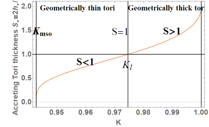
Analysis in Figs (16) shows that thickness is essentially regulated by the parameters and therefore the energy function . This analysis also sets the condition for the formation of RAD as a globulus, shows moreover classes of tori at equal of similar thickness therefore having similar properties which are essentially determined by this parameter as some aspects of the oscillations, it is clear also the role of critical limiting curves . Condition , showed in Figs 12 is a peculiar aspect of thick disks the limiting value (for accreting tori) is for , while the most general relation is shown in Figs 12 from which we see that in general for large and small there is , Figs 12 also show that the only a limited portion of discs in the conditions to be cusped satisfy the condition in general for small values of .
III.2.2 Formation of the outer torus in the marginally collision sphere:
The conditions for the emergence of the tori collision is important to establish the stability conditions of the RAD including misaligned tori and also possibly the time scale of the involved processes that are potentially observable66 6 The analysis of collisional spheres is also relevant for setting constraints for the observation and recognition of a black hole in the conditions considered here and also clarifies the perspective of the accretion ball, maximum BH coverage i.e. that condition for which BH is in suitable conditions and a stage in its life surrounded by accreting tori considered here. This limiting condition fixes in comparison with other embedded BH models as, for example, self gravitating shells. We consider now the condition , featuring the existence of an inner torus in accretion and a quiescent outer torus on a collision sphere (a sphere centered in the attractor and located at radius ). To this purpose we introduce the useful limiting radii
| (29) |
representing the conditions with the potential and therefore set limits for location of the inner and outer edges of quiescent tori with . Figure (18) shows the limit for the existence of these specific radii.


Figs (18) show the analysis if tori spacing for a couple of tori, where is the inner edge of the outer torus of the couple and is the outer edge of the inner torus of the couple with respect to the central BH, therefore this is substantially an analysis of the emergence of tori collision according to the state, cusped or quiescent tori and others morphological features. We can precise this relation considering the limits on the fluids angular momentum. From Eq. (29) we obtain the limiting specific angular momenta
| (30) |
where has been obtained using Eq. (28) in , represented in Figs 18 and 12. The function provides the specific angular momentum of the outer torus to have , where is the outer edge of the cusped torus (therefore ), defined in Eq. (28) and pictured in Figs 18 and 12. The inner edge is the limiting value for the inner edge location at , which is the -parameter of the outer torus being the superior limiting value of Eq. (30) and showed in Figs 18 and 12, relating the angular momentum of the inner and outer torus. Note that condition implies that there is only one value for the outer torus with inner edge equal to the outer edge of the inner accreting torus. In Figs 12 , or at the limiting conditions on the outer and inner edge of the cusped torus and for . is or the limiting value of the specific angular momentum (for ) at the outer edge of the cusped torus.
In general, the inner edge of the outer torus has to be , represented in figure Fig (18) (light-blue band) and we consider a restriction of this region due to the condition (corresponding to condition ). The limiting case occurs for of Eq. (30) with , (or such that ). It is clear that the larger is , the greater is the dimension of the outer torus. The other necessary condition is ; if the inner torus is cusped, then we can eliminate the dependence from the density parameter . Therefore, we consider the following two conditions in this special case: (a) The torus is cusped: , obtaining the relation ; (b) The inner torus is not cusped (quiescent phase): there is then , obtaining the relation . Note that eventually, in the (a) and (b) cases, we could search for a relation in terms of -parameters as a relation . We also obtain the following limits on the inner and outer radius:
where
| (31) | |||
| and | |||
| (32) | |||
| (33) | |||
| (34) | |||
| (35) | |||
| (36) |
Notice, and are the outer and the inner edges of the inner cusped torus, and (, ) are both the of the cusped torus, where and are in Eqs (12), while are defined in Eq. (16), and is in Eq. (14). We introduce the parameter as
| (37) |
which is the value of the -parameter at the center of torus, , or the value associated to the cusped tori, expressed as the function of intended as center or the inner edge of the cusped torus. The existence of a saddle point for at has implications on the density of the RAD tori structure (see analogue argument for in ringed; long). Thus there is also
| (38) |
considered as function of , for the center to have the outer torus located on the outer margin of the inner accreting one, i.e. (this can be obtained from Eqs (14) and (28) assuming ). Therefore, there has to be . The center of cusped torus is located in , whereas the outer edge can extend to very large distance from the attractor. For the analysis of this case, we return to the (AC)-model of Fig (11) modifying some definitions. Specifically, we introduce the specific angular momentum for case (1) , such that for there is and, asymptotically, for , there is . These new definitions restrict the analysis to cusped tori or quiescent tori in the angular momentum range . In Figs 19 we considered case (2)– the momenta such that, for , there is and, asymptotically, for , there is , finally in case (3), there is the specific angular momentum , being for , and for . Therefore we studied the momentum such that , the location of the torus center .


In the following section we will reconsider models associated with these for the evaluation of the quantity of each torus that are related to the energetic and depend on the thickness of the disks flow.
IV RAD energetics and limiting open surfaces for misaligned tori
A BH and especially a SMBH can be characterized by unusual or extraordinary periods of activity of the BH, in terms of enhanced accretion rates and interrupted accretion periods and jet emissions, detectable in the alteration of the mass accretion rates, or recognizable as mechanism at base for high masses considered in the SMBH, with a contribution of matter in accretion that one can think maximized by the number of accreting orbiting tori . Accretion, in the case of a globular model would prompt a relatively fast collapse of the structure into the central BH with a huge mass spin contribution, with a great release of energy and matter outburst. The RAD energetic quantities show two kinds of fundamental properties typical of geometrically thick disks. There is an explicit dependence of on the polytropic index and polytropic constant but as shown in Table (2) with an factors allowing to define independent quantities and therefore study the quantities E varying P, and therefore with respect to the morphological characteristics (quantities in Table (2) are re-parameterizations of respectively). This has an important consequence from the point of view of observation and recognition of such systems. Many characteristic studied in Sec. (II) and Sec. (III) are thus independent from details on the specific polytropic but rather consequences of the geometry and pressure gradients. These tori are therefore determined by the title angles-Figs (23).
As discussed in Sec. (II), the model adopted for the single toroid of the globulus, described as solutions of Eq. (2) with a barotropic equation of state, provides open-cusped surfaces whose meaning is yet to be fully understood. These special surfaces are associated with instabilities (in this case referred to as a topological features of the surfaces) having a broad centrifugal component with , and the cusp is located in a specific annulus externally with respect to the accretion cusp region–Figs (2). Therefore these structures, variously related to jet or proto-jets configurations are not directly correlated to accretion. It is clear then that the centrifugal component in competitions with the attractive gravitational component of the force balance equations, prevails although not sufficiently hight with respect to a strong gravitational component to stabilize the disk (absence of a cusp) as it occurs for the tori with specific momentum in . In Sec. (IV.1) we consider more specifically the polytropic fluids and the globuli characteristics directly dependent.on the polytropic parameters typical and in particular from the characteristics of the RAD energetics as the accretion rates.
IV.1 Polytropic fluids and RAD energetics
These RAD structures pose the interesting question of the internal activity of the cluster and particularly the internal exchanges of energy and matter between the tori and the tori and central BH. As considered for the eRAD system, RAD and globuli are characterized by a vivid internal activity made up of collision among tori, inner accretion, internal jet launch, whether constrained by open-proto-jet configurations considered here in Sec. (IV.1) or rather by jet emission from accretion jet correlation. This situation in case misaligned tori considered here is even more clear, the internal activity can eventually even undermine the structure and its stability especially in the case of Kerr attractor. The existence of these structures shows the possibility that a BH-system can be "dormant", quiescent, i.e. undergoing a period of low activity intended interactions with clouds, stars of BHs companions or more generally with the galactic environment. We could picture this situation defined cold or warm globulus otherwise the last having a vivid internal life and exchanges of energy and matter. One essential difference with respect to other similar situations foreseen embedded BH considered in the literature is the fact that we consider an orbiting non-self gravitating RAD composed by objects with very different characteristic starting from an intricate multipoles structure. In this section we provide evaluations of quantities related to tori energetics such as the mass-flux, the enthalpy-flux (evaluating also the temperature parameter), and the flux thickness–see abrafra; Japan–Table (2). Considering polytropic fluids with pressure , we listed these quantities in Table (2). These quantities have been obtained by considering the flow thickness expressed through the density profiles. The relativistic frequency reduces to Keplerian values at the edges of the accretion torus, where the pressure forces are vanishing 77 7 It has been shown that for the Schwarzschild geometry there is a specific classification of eligible polytropics (see Raine), and a specific class of polytropics is characterized by a discrete range of values for the index mnras.
| Quantities | |
|---|---|
| [-quantities]: | [-quantities]: |
To simplify this analysis we consider the general form or form, as in Table (2), where and are general functions of the polytropic index and polytropic constant . These quantities express the mass flow rate through the cusp (mass loss, accretion rates) , and the cusp luminosity (and the accretion efficiency ), measuring the rate of the thermal-energy carried at the cusp–seeabrafra; Japan; Blaschke:2016uyo; 2017PhRvD..96j4050S also long; Multy; Letter. The depend on the accretion sphere (inner edge of the cusped torus) and the radius which is related to the flow thickness, , of the matter flow. These quantities regulating the tori energetics are shown in Fig. 22 as functions of the cusp locations where the radius in the definitions of Table (2) has been fixed arbitrarily, preserving the geometric sense of this cut-off, and the dependence of the polytropic index through (polytropic index )–Figs 21:
| (39) |
where
| (40) |
and there is
| (41) |
(Note, models defined in Eq. (39), similar ti (AC) of Sec. (III) but defined through the evaluation of points setting and , setting and , as in Figs 21.)


Figs (21) shows the parameters relevant for the analysis of the energetics of the RAD; here we relate the parameter to the polytropic index. We should note that although we selected specific functional relations (curves in the figure) one has to consider the possibility to fit the observational data for a wide range of deducted parameter value, radial distances are relatively small in terms of mass of the central object and finally we are concerned here with the behavior of the curve with the variation of the parameters which provides a relative comparison with tori components. In the evaluation of these quantities considered in Figs 22 we considered chosen so that there is to ensure a non-zero flow thickness. The limiting quantities, as , have been evaluated assuming and , as is the limiting (maximum) distance, and we have assumed that may approach the horizon–Figs 21.


Figs (22) focus on the dependence of the energetics quantities on the polytropic equation of state and location of inner edge. This analysis therefore has to be compared with results of Sec. (III.1), and these considerations turn in terms of parameters analysis P in Figs (3,4), to the correspondent tori as objects of the curves in figures, characterized by a selected values E. This comparative analysis of Figs 21 and Figs 22 allows the study of quantities in dependence on the distance of the toroids from the central black hole and with variations of and .
V Discussion and Conclusions
The main topic of this paper is the analysis of the set of accreting tilted tori around the central BH. We studied clusters of misaligned (inclined) tori (RAD) orbiting one central Schwarzschild attractor. For this purpose we have defined the toroidal components of the gravitating system as an aggregate of misaligned perfect fluid tori orbiting the central Schwarzschild black hole using the approach developed in ringed; open; dsystem from the eRAD model construction. We stress that by considering a generic tilt angle we provide indication on the characteristics and observational properties for the clusters of orbiting tilted tori rather then an analysis of the single toroidal component of the aggregate. Constrains on existence of such configurations are discussed in Sec.(II.2), and particularly against tori collision in Sec. (III.2) and Paczynski instabilities– Sec. (II.1). We studied the BH-RAD energetics, Sec.(IV.1), and an overview of possible phenomena associated to the RAD structures, as possible proto-jets emerging in the RAD structure. Many morphological and stability properties (presence of the cusp) of the torus discussed Sec. (III) are constrained by the distance of the torus from the central attractor and regulated by the centrifugal component of the force balance inside the torus, therefore the disk rotational law. From methodological view point we take advantage of spherical symmetry providing the results for perfect fluids. Our analysis places constraints on the existence and stability of misaligned tori which can be used in dynamical (time-dependent) analysis of a similar system with these (evolving) initial configurations. With respect to the current literature considering similar objects within a numerical approach we frame the analysis in a fully analytical RAD models identifying one leading function to describe the distribution of tori. We singled out definition of RAD leading function of Eq. (3), the RAD energy function of Eq. (4). The outcomes of this approach results in constraining the inner structure of the RAD and tori morphological characteristics.
More in details: in section (II) we give the basic equations for the description of this system providing the RAD leading function governing the tori distribution in the orbiting macro-structure. We have therefore studied the model characteristics on the basis of the parameters determining the particular configurations according to their stability as related to the toroids morphology. We integrated the force balance equation for the equi-density (equi-potential) surfaces. The evaluation of the toroids geometrical thickness has an essential role in the evaluation of the effects of disc-seismology as clarified in next. Then geometry of RAD accreting tori, stability and collision emergence are focused in Sec. (III). This analysis also led to determine the misaligned tori collisional emergence. Here we provide the tori distributions in the RAD considering the characteristic of the geometric thickness and an evaluation of the geometric thickness of the disks considered in the RAD frame establishing conditions under which disks are geometrically thick according to the model parameters and the limit value . This analysis identifies the sets of RAD inclined toroids having equal or other characteristics as the torus thickness. The relevance of this analysis lies in the fact that the classes of toroids and therefore of RADs so classified might correspond to observational effects dependent on the characteristics R or which are similar (as we have seen in some cases in this work), thus it is important to model this type of toroids. We consider particularly the torus elongation , the location of the inner edge, the location of the torus center , corresponding to the point of maximum density and hydrostatic pressure, the location of the maximum , giving RAD tori maximum density and the torus thickness . These conditions are significant to establish the stability of the RAD including misaligned tori and also possibly the time scale of the involved processes that are potentially observable and which depend on the distance (spacing) between the toroids and their thickness, on the presence or absence of a cusp. More generally, the toroidal geometrical thickness is also an indication of the accretion disk model and BH accretion rates correlation. Then the presence of multi orbiting structures could influence the accretion rate of the central BH. Therefore, in Sec. (IV.1) we evaluated quantities related to tori energetics such as the mass-flux, the enthalpy-flux (evaluating also the temperature parameter), and the flux thickness depending on the model parameters for polytropic fluids. We discussed also the variation of these quantities depending on the distance from the source. The RADs are therefore characterized by a special and distinctive ringed structure that, as pointed out in ringed; long; dsystem, could be evidenced in the X-ray emission spectrum and as an imprint of the discrete inner RAD composition, or in the combined oscillatory phenomena associated to the tori model observable for example by the X-ray observatory ATHENA88 8 http://the-athena-x-ray-observatory.eu/. As a sideline of the present analysis, we also discussed some aspects of RAD models including proto-jet that can offer interesting scenarios as associated to misaligned tori, aligned along the toroid rotational axis, and therefore inclined with respect to the other toroidal components of the aggregate. Misaligned disks investigation faces aspects of the accretion disk formation after different processes, where misalignment can provide description of the early phases of formation of the RAD tori and probable means to justify the origin of counterrotating tori of the RAD. More generally, the analysis presented here has a natural extension in the study of the situation for the Kerr attractors, the co-evolution of central BH with the disks and influence of magnetic fields. In a broader perspective of analysis we should note that disk misalignment is expected to depend significantly on the central BH spin and particularly the dragging of frames has a determinant influence on the morphology and equilibrium of an accretion disk and this has also a notable importance in the misalignment. Magnetic fields then have a different role in determining the initial tori inclination of the disk, possibly supported by the flow dynamical pressure from the Lagrangian points, we will also focus in next on the case when the leading RAD function, defining the distribution of tori in the RAD with misaligned disks has changed to an alternative definition to include the effects of toroidal magnetic field. Part of our analysis was also dedicated to an evaluation of the disk geometry (specifically its thickness) which is crucially significant in many aspects of the accretion disk physics and phenomenology. In particular in next we focus on a more specific analysis of the role of geometrical thickness in relation to the disco-seismology effects for each toroid. In Sec. (III.2.1) we evaluated the conditions for which these can be considered geometrically thick.
In this frame we note here that this model envisages also the possibility of a static BH “embedded” in a set of orbiting RAD tori–as accreting globules–with the BH horizon “covered” to an observer at infinity, with the RAD representing a matter covering the central BH–see for example Figs 8,7,20. However, in this situation it remains to discuss the stability of these static BHs immersed in the set of accreting RAD tori. In the development of such possibility there are further aspects to be considered as, for example, the tori self-gravity99 9 A related interesting possibility of this model might consist in having a micro-BH embedded in a RAD. Micro-BHs are (hypothetical) black holes, possibly with a cosmological origin (primordial micro-BHs), which are essentially regulated by an important quantum mechanics role. An essential aspect of these objects is related on the possibility that they could evaporate through Hawking radiation process implying elementary particles with a radiation rate that is as larger as the minimum is the size of BH (eventually leading to BH explosion). The proposed model may naturally enter in the family of different models foreseing for example micro-BHs immersed in neutron stars. In our case we do not consider the tori self-gravity. Moreover it is essential to establish a mechanism for the formation of such tori orbiting a micro-BH. A further interesting aspect of this possibility is the combination of matter dynamics surrounding the central BH and the BH dynamics itself as for example the radiation emission from the BH together from jet emission from accreting configurations or the combination of the oscillation modes of the tori. These BHs where the accretion is absent would be surrounded by a empty region of minimum radius , located between between and , with the perimeter of the accreting inner edge in . This system could provide an interesting combination of classical and quantum effects. (Note the primordial black holes of initial mass around the grams would already be evaporated. Larger masses BHs could now be observed through the emission of rays associated to their activities). We note, however, that such BHs in the final stages of evolution may no longer be described as as a classic black hole. . An interesting aspect of the eventual presence of these spherical globules (on static attractors) would be the presence of the differently oriented spins orbiting tori. The tori instability can lead then to a collapse with very high energy release. The globulous assumption clearly implies a frozen (not dynamical) situations for at least a significant time scale in the attractor life, where the central black hole can be still considered spherically symmetric. The possibility that such globulous exists in a frozen state has to likely feature small or zero BH spin, and tori orbiting at large distance from the attractor (depending on , and , where is the Kerr BH spin and are Boyer–Lindquist coordinates pugtot) to reduce the dragging effects from the center spinning attractor that would imply the evolution in configurations with torsion of matter due to the Lense–Thirring effect. The unstable phases of the globules would be associated to great energy release, with BH accretion rates being approximately the sum of the accreting tori rates considering however the possible collisional effects, that could also lead to phases of interrupted accretion–see Sec. (IV.1). Among other possible observational effects that could be associated with these structures, we mention the possibility to observe tangled luminous anuli, shaping the accreting RAD inner structure essentially related to the RAD inner edge, supposed to be the most active part of the accreting disk. (For a more accurate analysis of optical effects see for example KS10; S11etal; Schee:2008fc; Schee:2013bya). On the other hand, the zones of tori collisions with wide angle separation (in particular orthogonal tori) are the surfaces areas . These regions, two for each pair of colliding tori, could appear as active (unstable) “bright knots”. The knot formation phase could be totally or partially overlapped with the formation phase of one or both RAD tori of the configurations. Such bright (active) knots have a radial separation (linear distance) and can be evaluated as maximal at , (for a maximum crossing) being the location of the inner edge of the torus of minimal area. Moreover, more generally the velocity difference between the fluids streams in the knots and between these and the torus may produces a shear effect triggering some kind of instability. These instabilities eventually may grow into material that (periodically) accretes on the configuration. The possible origin and evolution of such knotty structure is however closely related to the timescale of the processes related to knots. The dynamical timescales characterizing the knots should be considered in a dynamical model, considering explicitly the collisional effects.
We conclude summarizing the main aspects of the model setup and discussing the possible RAD associated phenomenology. We also mention some topics arising from the analysis developed in this investigation that would be planned for future work, for example the analysis of the proto-jets colliding with tori in RAD and the introduction of the BH spin in this RAD set-up.
- -
The model setup
This analysis is grounded upon some assumptions. (I) Firstly we considered a central static BH, which is a convenient approximation as a first approach to the exploration of the misaligned tori in the RAD frame. (II) We then assumed a GRHD perfect fluid, which is particulary adapted to obtain constraints for the set of tori, especially for GRMHD initial configurations. On the validity of this assumption with respect to the more realistic case for example where magnetic fields are expected to play a relevant role or in dynamic model, is clear considering that the torus morphology well adapts to the configurations provided even at later time in the analysis made in the numerical GRMHD dynamical case. Many aspects here considered are therefore well described by HD approximation. (III) The third assumption of the model sup-up concerns the disk rotational law. This issue is a complex topic of the physics of an accretion disk, especially in the GRMHD-MRI frame, where the angular momentum distribution and angular momentum transport in the disk, is entangled to the mechanism of accretion and related to turbulence and the viscosity inside the disk. This is in fact a controversial aspects in accretion process, particularly for geometrically thin accretion disk. Here we faced this issue considering two main assumptions: (1) we adopted a Keplerian rotational law for the RAD leading function, in Eq. (3), that represents the angular momentum distribution for the RAD tori set; (2) For each torus of the cluster we have assumed constant. The choice of has an immediate geometric sense detailed in Sec. (II.1) being directly connected to gravitational part of the fluid force balance equation (the Euler equation) and the system symmetries. The rotational law is per-se arbitrary, but this assumption is supported moreover by the consistence with the von Zeipel results, and it is used particularly in the comparative analysis with the so called Bondi spherical accretion characterized by a disk slow rotation (sub Keplerian i.e. )–abrafra. The choice constant for each torus and therefore the torus parametrization with the value is a very convenient choice in the HD RAD macrostructure scenario, since here we are more concerned with the global issue the RAD structure, as the tori location in the cluster, the location of the maximum and minimum pressure points and other morphological characteristics, rather then the details of the physics of each torus. This assumption on the other hand is very well known and widely adopted. Indeed, more generally for geometrically thick configurations it is assumed that the tori are essentially regulated by effects of strong gravitational fields, considered dominant with respect to the dissipative factors and therefore having the major role in the unstable phases of the system. This assumption consequentially translates in the assumption on time scales of dynamical, viscouse and thermal processes characterizing the torus and translating in the form of fluid energy momentum tensor, the equation of state (and eventually the constitutive equations) having consequences clearly on the definition of the disk rotational law (centrifugal forces). This in turn grounded the assumption of perfect fluid energy-momentum tensor too. Therefore during the evolution of dynamical processes, the functional form of the angular momentum together with the entropy distribution depend on the initial state of the system only rather then on the less influential dissipative processes, leading essentially to an ad hoc momentum distribution inside the disk Abramowicz:2008bk. This feature constitutes a great advantage of these models which in fact result extremely useful and predictive . On the other hand, in these models the entropy is constant along the flow and according to the von Zeipel condition, the surfaces of constant angular velocity and of constant specific angular momentum coincide and the rotation law is independent of the details of the equation of state. We include further considerations on these surfaces with regard to the RAD fluid characterizations in Sec. (A.3). (IV) A further assumption concerns the system symmetries. A static spherically symmetric central Schwarzschild BH is assumed for this first analysis of misaligned tori cluster, secondly we assumed the fluid flow be toroidal (we have use the analogy with a magnetic-like orbiting multipole), obtaining RAD steady (or stationary) states which is the usual assumption to construct these toroids–see also pugtot.
- -
RAD associated phenomenology and observable characteristics
- –
-
Recognizing a RAD from an emission spectrum
From phenomenological viewpoint, the RAD unstable phases turn significant for the high energy phenomena, as especially related to accretion onto super-massive black holes in AGNs, as well as the extremely energetic phenomena in quasars observable in their X-ray emission, as the X-ray obscuration and absorption by one of the RAD torus. In this respect we should emphasize two principal observational aspects related to two typical accretion disks dynamics that, framed within the RAD scenario, provide interesting implications and patters to recognize these structures: first we mention the tori proper modes of oscillation for the misaligned tori clustered in the RAD. The radially oscillating tori of the ringed disk could be related to the high-frequency quasi periodic oscillations which are now observed in non-thermal X-ray emission from compact objects (QPOs). The second consequential element of the RAD structure consists in the jet emission from the tilted toroidal components of the RAD. Concerning the possible correlation with QPOs emission, which is considered in next the oscillations of each component are added to others and are pulsations of the RAD, and possibly the globule creating a rather distinct detectable emission spectra. This is a still unclear feature of the X-ray astronomy which has been largely related to the physics of accretion and more specifically to the inner parts of the disk. More generally RAD inner structure may be revealed by X-ray spectroscopy, as relatively indistinct excesses on top of the relativistically broadened spectral line profile S11etal; KS10; Schee:2008fc, where the predicted relatively indistinct excesses of the relativistically broadened emission-line components, arise in a well-confined radial distance in each toroid and the RAD.
- –
-
Recognizing a "globulus" structure
Globules are interesting from the observational point of view constituting in fact a possible BH embedding. The orbiting matter is a multipole-system characterized by the presence of different tori. It is in fact possible that these systems may be originated from different accreting periods of the central attractor life interacting with its galactic environment therefore being composed by matter with diversified characteristic. A globulus can be pictured as a configuration of very thick, Keplerian or super-Keplerian tori having angular momentum distribution equal or superior to in Eq. (3). This structure would cover almost completely the central embedded black hole. The BH horizon is then covered almost completely from the observer-view at different angles, as an embedding of gravitating orbiting matter around the BH. Hence the model would picture a EBH system, leading in fact to consider the BH-disk as one entire single object. (In this model we exclude the tori self-gravity). The dynamics of BH-disk system is in fact often considered in this unified picture for example in different approaches foreseing BH energy extraction from interaction with the surrounding orbiting tori or measurement of the BH spin by the analysis of the inner edge of the disk. A globulus would be recognizable by a series of main typical characteristics: (i) the first element typical of a globulous structure is the presence of an internal-globulus vacuum zone, the region in the range , where is the inner edge of the inner quiescent torus of the globulus and radial distance (in Boyer–Lindquist frame) is with respect to the central singularity. Of course if on the other had the inner torus is accreting, then this region would be characterized by the presence of matter accretion onto the attractor. The occurrence of this condition is thoroughly analyzed in this analysis considering , cusp location and conditions related such configurations. (ii) The system is characterized by a complex, specific "multipoles structure" (with "multipoles number" equal to for RAD toroidal components, so that it would be a dypole in the Schwarzschild BH case with one torus) characterized by the different (satellite) spins due to the different mislaigned tori rotation orientations and the central (primary) BH spin which in the case considered in this article is null. (In this article we consider more specifically a magnetic like multipole, the fluid having only a toroidal flow). (iii) The globulus is subjected to different constraints due to the emergence of tori collision. Such constrains reduce to conditions on the tori angular momentum, which is the value of model parameter characterizing each torus, a value of the RAD rotational curve , and tori morphology, here considered determined by a set of tori morphological characteristic as the torus geometrical thickness, height and elongation on the torus symmetric plane, emergence of cusp instability here largely considered Sec. (II) and Sec. (III), and other characteristics related to RAD-BH system energetics as the accretion rates or the cusp luminosity, considered in Sec. (IV.1). (Obviously in the case more specifically of globulus it is necessary to consider the constraints imposed by the regions in Figs (16,17) to identify each torus based on its geometric thickness, and Figs (13), thus deducing the conditions on tori parameters and tracing them through these constraints on their morphology). (iv) A peculiar feature relevant for the observation and recognition of the RAD and globuli particularly is its extension and location of the outmost torus of the orbiting aggregate. This issue has been addressed evaluating the constraints on the outer edge of the outer torus of the RAD, and more generally the limiting on the locations of maximum density point in the farthest torus , we mention particularly Sec. (III.2.2) and Sec. (A.3). (v) Finally the globulus would be recognizable by an articulated internal life triggered by each torus dynamics and empowered by the entangled, ringed inner structure, made up by a sequel of typical associated phenomena as tori collisions, tori oscillation modes (eventually related to QPOs emission as we have considered in next), and possibly internal accretions and jet emission.
- –
-
On the jet emission in the RAD
A further interesting aspect of the RAD multipole structure is the possibility that this may be reflected in the associated jet emission. Regarding the internal RAD jet emission, the possibility of an extended jet launching region has been widely considered for the eRAD model in open; proto-jet; dsystem; long. Jet emission in BH accretion disks system in fact can be equally considered autonomously from the occurrence of the open solutions with cusp, predicted in the perfect fluid tori considered here under special conditions on momentum and identified with "proto-jet".
The (multi-polar globules with) shells of jets in accreting balls, can have huge consequences for the RAD stability and observation and, possibly, having impact also for the galactic environment enrichment process. In the cluster frame presented here and more generally in the RAD frame, there are several points to be addressed concerning this intriguing aspects of the orbiting agglomerate.
Jet emission has been in fact largely directly connected to accretion and more specifically accretion disks and the inner regions of accreting disk. Although the issue of jet launch still needs to be resolved, a large part of the current analysis relates, at least geometrically, the inner edge of accreting disk to jet emission. Consequently, in this frame of the torus-jet emission correlation, we could consider the occurrence for each toroidal component of the globule, predicting accordingly the presence of inner RAD globulus jets, whose detection would be an indication on the presence of the RAD structure.
It should be pointed out that the orientation of the jet in the case of static attractor can be supposed to be orthogonal to the (torus) plane of symmetry resulting in the rotation (the dipole) direction, in the case of attractor with spin. We also know to be ascertained that the spin of the central attractor has indeed a role in the launch of jets, in the collimation and in the determination of the direction of the jet, together with the presence of the magnetic fields. The jets presence is a complex scenario that, if observed, would open an important observational window both on the determination of the physics of BH and on the understanding of process of energy emission. There are important aspects connected the HD proto-jets structures, associated to the energetics in the RAD tori environment. The analysis in ringed; open; dsystem; long, introducing the eRAD models, details the HD matter, multi-proto-jets in the Kerr SMBH spacetime having, therefore, also an initial (in the vicinity of the launch point ) counter-rotating component, and mixed corotating/counter-rotating funnels of material. In proto-jet we focused specifically on proto-jets configurations in eRADs orbiting a Kerr SMBH considering thoroughly the symmetries and limiting surfaces and highlighting the boundary limiting surfaces connected to the emergency of the jet-like instabilities with the black hole dimensionless spin. The energetics is addressed more specifically in Multy by concentrating on the energy released during collision and time-dependent accretion examined in the more simple example of situations where deterministic chaos might emerge, considering a modified accretion rate law. Then jet emission was considered in Letter with emerging tori collisions around super-massive Kerr black holes, providing an evaluation of center-of-mass energy for two colliding particles from the two interacting tori.
In future work we are planning to consider more specifically the impacts of the proto-jets with accreting tori in the RAD configurations as globules. In the case of Kerr BH, there can be the occurrence of a more external shell, "breaking" the internal accretion disk. This limiting occurrence, regulated by the background geometry and precisely by the Kerr BH dimensionless spin distinguishes also the torus direction of rotation–open; proto-jet; long. In the case of a spherically symmetric spacetime, this occurrence does not exist. Considering the shells in Fig. (2) and analysis of constraints in Sec. (III), there are completely separate and disconnected regions where these configurations can emerge, and yet in some of these it is still possible that interaction between structures with maximum density in different regions give rise to collision or possibly replenishment and exchange of matter. The outer region is associated to generally very thick tori with a large centrifugal component (with respect to the other components in force balance equation of Eq. (1)) and with the characteristics of energetics considered in Sec. (IV). This region is followed by the intermediate region of quiescent tori and proto-jet emission and the inner region with quiescent or accreting tori having lower density and momentum. This is obviously because in the case of a static central attractor the direction of rotation of the fluid is not diversified against the gravitational background. Noting that proto-jets are open, cusped solutions associated to geometrically thick tori as described by the model in Sec. (III) and open; Lasota:2015bii, we can expect that the associated toroidal fluid configurations provide eventually also the source material, and determining the initial prompting centrifugal component, especially in the HD model orbiting a static central attract.
Considering different "companion disk" models, this enlarged ground of elements affecting the proto-jets funnels can be enriched by the viscosity and resistivity terms which, as we have largely discussed in this analysis, in the context settled here for the constraints investigation, can be neglected in first approximation. Here we consider the limiting conditions on fluid centrifugal components and the general relativistic effects of a Schwarzschild background, using therefore an adapted HD model as base for the enlarged situation with a richer, more complex, embedding of accretion. On the other hand in many GRMHD analyzes the only HD has proved to be a good comparative pattern and certain a good initial condition.
However, in proto-jet we have the dragging due to the Lense–Thirring effect around a Kerr BH, affecting possibly both launching and collimation of the corotating and counterrotating component of the fluid and, at the same time, in the eRAD components the relative directions of proto-jet rotation is parallel or antiparallel in all jet shells. By imposing a static background, we have maintained the mutual co-rotation or counter-rotation of the funnels, but this possibility is now expanded including different relative angles of the rotation axes: consequently the proto-jets are no longer "parallel" or "anti-parallel", but they are always "orthogonal" to the rotation plane of the orbiting toroidal embedding material which eventually constitutes both the replenishment material and collision and centrifugal support.
Although proto-jets are expected to be somehow transient structures, the presence of the tori of RAD may constitute a reservoir materials and momentum to reform or enact possibly also associated to occurrence of runaway or runaway--runaway instability, constituting eventually interrupted sequences of complex outbursts with different shells and a structured orbiting disk. These solutions have been differently associated to jet emission empowered by initial unstable fluid centrifugal component associated to a minimum of pressure correspondent to the surface cusp. In these structures we proved that the centrifugal component should be not "too large" that the disk is stabilized against the formation of the cusp1010 10 We proved that proto-jets are associated to fluids having initial specific angular momentum with , therefore the cusp is located in an instability shell of radius located at from the attractor and separated by the photon sphere with . The center of maximum pressure is located in a shell of radius (). and are in fact "geometrically not correlated" directly with accretion where the accreting fluid has initial specific angular momentum lower then the fluid supporting proto-jet, whose cusp is closer to the BH then the accreting point. The proto-jet structure is a shell englobing the accreting configuration as shown Fig. (2) distinguishing these configurations from other open structures. It is possible that tori eventually formed in the condition for proto-jet as described here could more or less rapidly undergo a phase of angular momentum decreasing bringing the torus in the condition for accretion. The presence of proto-jet cusp is also regulated by the parameter, corresponding to mass and density term parameter, related to very large tori, hence the reservoir of mater and funnels. There could be the concomitant formation of internal proto-jet associated to an outer toroid and related to a disk between them, which is in accretion, replenishing also the cusp of the proto-jet. The fluid of the inner shell has a higher specific momentum of the intermediate shell where there is an accretion point and maximum pressure of the accretion disk, which then replenishes the jet with a fluid with initial lower moment. It is in fact clear that the replenishment fluid can have then a very diversified (with respect to the proto-jet funnel) initial rotation direction and matter properties component. We firstly propose that there are multiple, and simultaneously tilted, proto-jets with very different materials, and secondly we foresee the possibility of impact in the RAD of jet on disk which we plan to analyze with more details elsewhere. Therefore for a forthcoming paper we plan to extend this set up to consider in a clear and systematic way the jets and tori in schwarzschild geometry as well as tilted tori in an approximated Lense–Thirring geometry and the Kerr geometry.
- –
-
Outbursts and geometry perturbation triggered by RAD instabilities
The occurrence of the principal RAD instabilities initiates an interesting set of associated RAD phenomenology. The consequences of the RAD instability processes have to be considered in the analysis of energetic involving a SMBH interacting with orbiting tori. There are four main typical RAD instabilities which can lead to some kind of disruption or even catastrophic destruction of the RAD internal structure characterized by large and relatively fast release of matter and energy outburst triggered from the occurrence of tori accretion, tori collision or a combination of these two effects. We studied the energetics of BH accreting disk related to accretion phase in Sec. (IV.1) in functions of the model parameters, location of the cusps and distance from the central BH scaled with the BH mass . We include, in the discussion of RAD phenomenology, some further notes on the fourth RAD instability consisting in the runaway-runaway instability. The runaway instability has also been considered playing a part in the energy extraction from the central BH engine, the extraction of the rotational energy of the spinning black hole via the Blandford-Znajek mechanism, and in the GRB production. The runaway-runaway process, triggered by the occurrence of runaway instability prompted by accretion from the inner torus of the RAD induces also a change in the BH parameters, therefore changing the spacetime geometry and consequently changing the RAD structure. While the accretion from the inner torus may establish the runaway instability, this can be accompanied by a further process of torus-torus interaction, inducing the other instabilities processes. Such tori collision may go through a positive or negative feedback reaction, since the runaway mechanism is essentially an interactive process involving both the attractor and the accreting torus initially due to the interaction of the BH with the inner accreting torus via accretion of matter flowing into the BHs—-dsystem. If a runaway of the inner RAD torus is established, then also the outer torus of the RAD is affected. The runaway instability is regulated by several parameters, particularly the dependence of the mass accretion rate– here considered in Sec. (IV.1), the initial the cusp location–Sec. (III), the flow thickness–Sec. (III.2.1). Because of the change in the mass BH parameter, the accreting torus cusp can move deeply towards the torus, and increasing the mass lost rate due to the cusp will bend inside the torus, BH mass increases, according to the mass accretion rate. If the non-zero BH spin is constant during this process then this implies a decreasing the spin-to-mass ratio. A similar mechanism of BH-accreting torus interaction can arise also after a spin-shift for energy extraction for example, eventually the question if there is a phase of accretion process where the central (static or spinning) BH may acquire an electrical charge and the role of this phase in the subsequence phases of BH matter interaction is in fact still a wide open (not irrelevant) issue. A possible consequence of the entire process is however that the accretion tori and consequently the RAD never reach a steady state. Note that otherwise the accreting inner torus could even be completely destroyed by such instability. We should also note that, from the point of RAD morphology structure, the accreting torus cusp may also move inwardly i.e. towards the central black hole, with the consequent decreasing of the mass transfer, ending eventually in stabilizing the entire process. The runaway instability when the cusp moves outwardly, penetrating the torus, results in an increases of mass transfer rate. We considered the dependence of the accretion rate on the cusp location and other parameters in the analysis of Sec. (IV.1). It is worth to point out however how the study of this situation has been carried out by considering stationary models Font02, in a non-dynamical framework and therefore particularly adapted to the RAD scenario constructed here. In this approach the evolution of the central black hole is described as a sequence of exact black holes solutions with a different mass, function of the mass accretion rate of the former state. Pictures of the systems during stages of its dynamics were studied, this method was carefully analyzed and discussed for geometrically thick torus around Kerr BHs in pugtot. Finally we note that a relevant factor of this process especially in the RAD frame, where there is the combination several processes and dynamics, consists in the typical time-scales that should be compared with the time-scale of the dynamical processes of the accreting torus and RAD dynamics.
Misaligned disks are usually located, by observational evidences, in AGNs at relatively large distances from the central SMBHs 2006MNRAS.368.1196L; Herrnstein1996; Greenhill2003. A warped inner accretion can explain the relation between radio-jets in AGN and the galaxy disk. Evidences of misalignment and details on observational expectations of the structure of tilted disks and proto-jets are discussed for example in Miller-Jones:2019zla. These investigations are focused on relativistic jets in a stellar-mass black holes launched and "redirected" from the accretion and subjected to the frame dragging effect. Others are more focused on the images of accreting black holes in presence of the disk and jet misalignment Chatterjee:2020eqc, developed by 3D relativistic MHD simulations 2011ApJ…730…36D; Fragile:2008sv. Many of these investigations address particularly the flow structure and the inner region of the tilted disk KKK; LLL; Teixeira:2014una.
Therefore, observational data concern more accretion periods of SMBHs located in AGNs, leaving traces in counterrotating and even misaligned structures orbiting around the SMBHs. RADs might represent the episodic accretion phases with different evolutive patterns apite1; apite2; apite3; Li:2012ts; Oka2017; Kawa; Allen:2006mh, grounding the process of accretion for SMBHs from intermediate or low mass BH seeds (), especially at cosmological distances with redshift . These structures would be recognizable from the long and continuous accretion episodes due to tori merging, and eventually involving also a relevant spin-shift and a succession of accretion episodes from misaligned disks, characterized by a sequence of turning-on and turning-off of super-Eddington accretion phases to sub-Eddington phases. The implications and potential observational consequences of the new results connected to RAD analysis developed here reside on two different sides. Firstly, the results base the analysis of the peculiar limiting effects developed in next where the implications of the RAD structures in QPOs emission are analyzed. Further peculiar object associated to the RAD morphology is the orbiting globulis covering the central BH, a limiting situation that could give rise to a huge release of energy due to the unstable modes, with a complex structure injecting matter collapsing onto the central attractor. In the simulation and observation of more complex systems in evolution, we would recognize the constraints derived by quantities easy reducible to the parameter set considered here. In these complex systems constraints would appear, resulting from the analysis of Sec. (II.2) and Sec. (III) evaluating the GRHD effects.
As previously stated, one of the future targets of this analysis is the extrapolation of the results and analysis developed here for the rotating background case represented by a central Kerr SMBH. In Sec. (I) we discussed the role of Schwarzschild limit as a first-step analysis for the spinning case. The exploration of the static geometry case is indeed useful to discern the Lense–Thirring effects on the disks with respect to other factors contributing to the disks dynamics. As noted in dsystem for the eRAD in Kerr spacetime, the inner ringed structure is different, in relation to the classes of different spin-mass ratios of the central attractor, for the set of corotating and counterrotating tori as related to the attractor, and for the corotating and counterrotating sequences. For all these reasons the analysis of the Schwarzschild backgroundg serves as comparative test and first analysis step for more complex situations, for the extension to Kerr background and comparison in different situations determined also by different characteristics of the disk.
Acknowledgements.
D. P. and Z. S. acknowledge the financial and institutional support of the Institute of Physics, Silesian University in Opava. Z. S. acknowledges the support of the Czech Science Foundation grant 19-039505.Appendix A Further notes on tori construction and limiting configurations
A.1 On and functions
In this section we briefly discuss some geometric and dynamic aspects underlying the definition of the specific angular momentum adopted in Eq. (3) and energy function of Eq. (4), focusing on their geometric origin related to the symmetries of the Kerr background. The significance of quantity (3) for the extended matter in orbit in the RAD context is then explored. For this purpose we start by considering the Schwarzschild metric
| (42) |
written in standard spherical coordinates . It is convenient to list here the following quantities
| (43) |
the -quantities are the four fluid velocity components and -quantities are the constants of motion for test particle geodesics with four-momentum , which are related to the Kerr geometry Killing vectors and . From and we define the following quantities , together with the relativistic angular frequency and the fluid specific angular momentum for Eq. (3):
| (44) |
Assuming , for the circular configurations, there is from Eq. (44), and we obtain explicitly
| (45) | |||
| (46) |
In Eq. (45) is the effective potential expressed in terms of , constant of motion for test particles in circular motion, and we included explicit dependence on the poloidal component of the fluid velocity , while in Eq. (46), indicated as function of as in Eq. (44). In the clusterized set of misaligned tori, using the background and the toroidal disk symmetries, we can consider, without loss of generality, the condition (equivalent to ) for each toroidal component of the cluster reducing, for each toroid Eq. (45) to Eq. (44). Within our assumptions , from the Euler equation (1) we obtain the expression for the radial pressure gradient, regulated by the radial gradient of the effective potential which provides the integral form Eq. (2). It is then convenient also to define the following angular momenta
| (47) |
where is the angular momentum defined in Eq. (43) as constant of for test particle circular motion, regulated by the effective potential in Eq. (45). In Eq. (47) expresses as function of the fluid specific angular momentum as in Eq. (44) (clearly for very large radius there is ), we note that exists for . In Eq. (47)- we give the fluid specific angular momentum of Eq. (3) with the explicit dependence on the BH equatorial plane. In figure (25) and Appendix (A.3) we discuss further properties of these quantities.
A.2 Toroidal surfaces
The analysis of the tori equatorial sections, and the morphological characteristics of the associated toroidal constant pressure and density surfaces given by Eq. (1), allows to deduce important properties for the constraints on the orbiting tori cluster. From Eqs (1) we obtain the following expression for the toroidal surfaces on each plane :
| (48) |
where , and are functions of cartesian coordinates on an equatorial plane, for example we have fixed in Figs 8,23–where are Cartesian coordinates.


We now introduce the following limiting surfaces:
| (49) |
( is the absolute value of , and gives the complex conjugate of ) obtained from Eq. (48) where of Eq. (3). These limiting configurations have a significant number of symmetries. We describe these properties by referring to the Fig (24), the solutions for and . Surfaces in Eq (49) represent limiting solutions for the existence of the toroidal configurations, providing the maximum and minimum limits on the inner edge of the associated rigid toroidal surfaces.


A.3 On the upper limit on the RAD (globule) radius
The issue of the RAD (globulus) extension is correlated to two important consequential aspects of the RAD structure, the existence of the limit on the RAD mass and radius, as well as on the spin of the orbiting extended multipole object. Eventually one can consider a cluster of RAD where the outer tori has a preeminent role in the determination of a possible RAD collision with another element of the cluster. However, constrains on the existence of such limit can be provided by factors which are actually external to the model setup considered here, for example due to the other factors regulating accretion disks and accretion processes as presence of magnetic fields or also from the BH interaction with its host environment usually a galactic embedding. This last aspect requires clearly a focus on the characteristics of the typical RAD environment. It is possible that clusters of orbiting globules and clusters of clusters could be formed in some eras of BH formation and especially in low activity periods characterized by minor interaction of the central BH with its host for example in the (rather rarefied) galactic environment. The gravitating shells of tori could constitute a frozen situation in which the center BH would be inert and isolated in particular circumstances (cold RAD). Otherwise the presence of small spins, would induce BH globuli collision followed by very violent destabilization effects. Firstly a RAD radius definition may be well established as the outer radius of the outer torus of the RAD, this radius has been studied and constrained in Sec. (III). Particularly we refer to Eqs (24,12) and Figs (10,11), for accreting configurations in Eq. (24)–Figs (13) and Eqs (28,30)– Figs (18,12,9). Considering also the torus elongations (which sets the problem of inner edge location) there is Eqs (10)–Figs (9,10,11,12,13) and Eq. (29)–Sec. (III.2.2), Eqs (30,37)– Figs (18,12). For start we can set the most external torus in the region , and therefore with . (Note this implies a constrain on the maximum density point and the outer edge but not on the inner edge of the outer disk, which can in fact be also in , the detailed analysis of this issue for eRAD Kerr attractors and its Schwarzschild limit for corotating or the more probably outer counterrotating tori can be found in open; long). For these tori, for large , the prevalence of self-gravity of the thick configuration can be indeed a consistent factor regulating the structure. A further limit may originate by constrains on the magnitude of the relativistic angular velocity , which is a further relevant point for the fluid and disk, and toroidal fluid velocity, , which can be found here from , as in Eq. (44), and related to the (constant) von Zeipel surfaces. These quantities are related in Eqs (47), we refer also mnras for a careful study of these related quantities in the Schwarzschild spacetime, however below we provide for convenience some further notes on these elements.
Therefore we consider here again , and , obtaining
| (50) |
is the curve of the relativistic velocity evaluated on the RAD rotation curve, defines the surface of von Zeipel which we consider in Figs (25). We analyzed the asymptotic regime for large
| (51) | |||||
| (52) |
The form of the rotational law for large evidences the existence of the maximum density point . However the presence of a central BH spin, a condition which is to be considered highly probable, modifies the location of this radius with respect to the corresponding spheres of stability and therefore has important consequences from the point of view of the formation of these globular tori at large distances. In the case of Kerr attractor besides, there is the further issue of the role of counter-rotating discs (in the eRAD case this are obviously well defined, in the RAD we intend the counterrotating component of the torus spin with respect to the Kerr BH) that would be the most likely to be formed in the outer regions– dsystem; long; Letter; Multy


References
- (1) J. M. Bardeen, J. A. Petterson, Astrophys. J. 195, L65 (1975).
- (2) R. G. Martin, C. Nixon, S. H. Lubow, et al. Astrophys. J. 792, L33 (2014).
- (3) A. King and C. Nixon, Astrophys. J. 857, 1, L7 (2018).
- (4) C. Nixon, , King, A., Price, D., et al., Astrophys. J. , 757, L24 (2012).
- (5) C. J. Nixon, A. R. King, & D. J. Price, MNRAS, 422, 2547 (2012).
- (6) R. Nealon, D. J. Price, & C. J. Nixon, MNRAS, 448, 1526 (2015).
- (7) G. Lodato & J. E. Pringle, MNRAS, 368, 1196 (2006).
- (8) P. A. O. Scheuerl& R. Feiler, MNRAS, 282, 291–294 (1996).
- (9) A. R. King S. H. Lubow G. I. Ogilvie J. E. Pringle, MNRAS, 363, 49–56 (2005).
- (10) D. Pugliese& G. Montani, Phys. Rev. D, 91, 083011 (2015).
- (11) D. Pugliese& Z. Stuchlík, Astrophys. J. Suppl., 221, 2, 25 (2015).
- (12) D. Pugliese& Z. Stuchlík, Eur. Phys. J. C 79, 4, 288 (2019).
- (13) D. Pugliese and Z. Stuchlík, Class. Quant. Grav. 35, 10, 105005 (2018).
- (14) D. Pugliese, G. Montani & M. G. Bernardini, MNRAS, 428, 2, 952 (2013).
- (15) D. Pugliese& Z. Stuchlík, Astrophys. J. Suppl., 223, 2, 27 (2016).
- (16) D. Pugliese& Z. Stuchlík, Astrophys. J. Suppl., 229, 2, 40 (2017).
- (17) D. Pugliese & Z. Stuchlík, JHEAp 17, 1, (2018).
- (18) D. Pugliese & Z. Stuchlik, Class. Quant. Grav. 35, 18, 185008 (2018).
- (19) D. Pugliese& Z. Stuchlík, Mon.Not.Roy.Astron.Soc. 493, 3, 4229–4255(2020).
- (20) N. Dadhich, A. Tursunov, B. Ahmedov, et al. 2018, MNRAS, 478, L89
- (21) A. Tursunov, Z. Stuchlík, M. Kološ, APJ. 895,14 (2020).
- (22) Z. Stuchlík, M. Kološ, J. Kovář, et al. 2020, Universe, 6, 26
- (23) C. Alig, M. Schartmann, A. Burkert, K. Dolag, Astrophys. J. , 771, 2, 119 (2013).
- (24) R. V. E. Lovelace& T. Chou, Astrophys. J. , 468, L25 (1996).
- (25) E. Gafton, E. Tejeda, et al MNRAS, 449, 1, 771 (2015)
- (26) J. M. Miller, et alNature (London), 526, 542–545 (2015)
- (27) P. K. Blanchard, et al., arXiv:1703.07816 [astro-ph.HE] (2017)
- (28) J.M. Carmona-Loaiza, M. Colpi, M. Dotti& R. Valdarnini, MNRAS, 453, 1608 (2015)
- (29) S. Dyda, R.V.E. Lovelace, et al MNRAS, 446, 613 (2015)
- (30) C. Nixon, A. King, & D. Price, D., MNRAS, 434, 1946 (2013).
- (31) S. Dogan, C. Nixon, A. King, D. J. Price, MNRAS, 449, 2, 1251 (2015)
- (32) C. Bonnerot,E. M. Rossi, G. Lodato & D. J. Price, MNRAS, 455, 2, 2253 (2016)
- (33) I. A. Bonnell, & W. K. M. Rice, Science, 321, 1060 (2008).
- (34) K. Zubovas, A. King,arXiv:1901.02224 [astro-ph.GA], (2008)
- (35) H. Aly, W. Dehnen, C. Nixon, & A. King, MNRAS, 449, 1, 65 (2015).
- (36) D. Pugliese and G. Montani, MNRAS, 476, 4, 4346 (2018).
- (37) J. Kovar, P. Slany, Z. Stuchlik, V. Karas, C. Cremaschini and J. C. Miller, Phys. Rev. D 84, 084002 (2011)
- (38) Z. Stuchlik, P. Slany, G. Torok and M. A. Abramowicz, Phys. Rev. D 71 024037 (2005)
- (39) J. Kovar, O. Kopacek, V. Karas and Z. Stuchlik, Class. Quant. Grav. 27, 135006 (2010).
- (40) P. Slany, J. Kovar, Z. Stuchlik and V. Karas, Astrophys. J. Suppl. 205, 3 (2013).
- (41) J. Kovar, P. Slany, C. Cremaschini, et al. Phys. Rev. D 90, 4, 044029 (2014).
- (42) C. Cremaschini, J. Kovář, P. Slaný , et al. 2013, Astrophys. J. Suppl., 209, 15
- (43) A. Trova, V. Karas, P. Slany and J. Kovar, Astrophys. J. Suppl. 226, 1, 12 (2016).
- (44) J. Kovar, P. Slany, C. Cremaschini, et al. Phys. Rev. D 93, 12, 124055 (2016).
- (45) A. Trova, K. Schroven, E. Hackmann, et al,. Phys. Rev. D 97, 10, 104019 (2018)
- (46) K. Schroven, A. Trova, E. Hackmann and C. Lämmerzahl, Phys. Rev. D 98, 2, 023017 (2018).
- (47) Z. Stuchlik, Bulletin of the Astronomical Institutes of Czechoslovakia, 34, 129 (1983).
- (48) Z. Stuchlík, & S. Hledík, Phys. Rev. D, 60, 044006 (1999).
- (49) Z. Stuchlík, P. Slaný & S. Hledík, A&A, 363, 425 (2000).
- (50) Z. Stuchlík, Modern Physics Letters A, 20, 561 (2005).
- (51) Z. Stuchlík, S. Hledík, & J. Novotný, Phys. Rev. D, 94, 1053513 (2016).
- (52) P. R. Brady, J. Louko, and E. Poisson, Phys. Rev. D 44, 1891 (1991).
- (53) N. M. Garcia, F. S. N. Lobo, and M. Visser, Phys. Rev. D 86, 044026 (2012).
- (54) F. S N Lobo & P. Crawford, Class. Quant. Grav. 22, 4869–4886 (2005).
- (55) J. Frauendienert, C. Hoenselaers and W. Konrad, Class. Quantum Grav. 7, 585–587 (1990).
- (56) M. A. Abramowicz & P. C. Fragile, Living Rev. Relativity, 16, 1, (2013).
- (57) J. A. Font, & F. Daigne, Astrophys. J. l, 581, L23 (2002).
- (58) D. Pugliese&G. Montani, EPL, 101, 1, 19001 (2013).
- (59) R. H. Boyer, MPCPS, 61, 527 (1965).
- (60) Q. Lei, M. A. Abramowicz, P. C. Fragile, et al., Astron. Astrophys., 498, 471 (2008).
- (61) M. A. Abramowicz, arXiv:astro-ph/0812.3924, (2008).
- (62) M. A. Abramowicz, M. Jaroszyński, M. Sikora, Astron. Astrophys, 63, 221 (1978).
- (63) J.-P. Lasota, R.S.S. Vieira, A. Sadowski, R. Narayan, & M. A. Abramowicz, A&A., 587, A13 (2016)
- (64) M. Blaschke, & Z. Stuchlík Phys. Rev. D, 94, 8, 086006 (2016)
- (65) Z. Stuchlík, M. Blaschke, & J. Schee, 2017, Phys. Rev. D, 96, 104050
- (66) M. A. Abramowicz, Astronomical Society of Japan, 37, 4, 727–734 (1985).
- (67) V. Karas& V. Sochora, Astrophys. J. , 725, 2, 1507–1515 (2010).
- (68) V. Sochora, V. Karas, J. Svoboda, & M. Dovciak, MNRAS, 418, 276–283 (2011).
- (69) J. Schee& Z. Stuchlik, Gen. Rel. Grav., 41, 1795 (2009).
- (70) J. Schee & Z. Stuchlik, JCAP 1304, 005 (2013).
- (71) Abramowicz, M.A., Jaroszyński, M. & Sikora, M. 1978, A&A, 63, 221
- (72) J. Frank, A. King, D. Raine, Accretion Power in Astrophysics, (Cambridge University Press, Cambridge 2002)
- (73) H. Bondi, MNRAS, 112, 195 (1952).
- (74) J. A. Font, & F. Daigne, MNRAS, 334, 383 (2002).
- (75) J. M. Bardeen, J. A. Petterson, Astronomy & Astrophysics Letters, 195, L65 (1975).
- (76) R. Nealon, D. Price and C. Nixon, Mon. Not. Roy. Astron. Soc. 448 no.2, 1526 (2015).
- (77) M. Bugli, J. Guilet, E. Miller, Mon. Not. Roy. Astron. Soc., 475, p. 108 (2018).,
- (78) B. Paczyński, Acta Astronomica, 30, 4 (1980)
- (79) B. Paczyński, astro-ph/0004129 (2000).
- (80) J. R. Herrnstein, L. J. Greenhill, J. M. Moran, ApJ, 468, L17 (1996).
- (81) L. J. Greenhill, P. T. Kondratko, J. E. J. Lovell, T. B. H. Kuiper, et al., ApJ, 582, L11 (2003)
- (82) K. Chatterjee, Z. Younsi, M. Liska, A. Tchekhovskoy, S. Markoff, D. Yoon, D. van Eijnatten, C. Hesp, A. Ingram and M. van der Klis, [arXiv:2002.08386 [astro-ph.GA]].
- (83) J. C. Miller-Jones, A. J. Tetarenko, G. R. Sivakoff, M. J. Middleton, D. Altamirano, G. E. Anderson, T. M. Belloni, R. P. Fender, P. G. Jonker, E. G. Körding, H. A. Krimm, D. Maitra, S. Markoff, S. Migliari, K. P. Mooley, M. P. Rupen, D. M. Russell, T. D. Russell, C. L. Sarazin, R. Soria and V. Tudose, Nature 569 (2019), 374-377
- (84) J. Dexter & P. C. Fragile, Astrophys. J. , 730, 36 (2011).
- (85) P. Fragile and O. M. Blaes, Astrophys. J. 687 (2008), 757.
- (86) A. Franchini, R. G. Martin, S.H. Lubow, MNRAS, 485, 1, 315–325 (2019).
- (87) simulations of tilted thin accretion discs M. Liska, A. Tchekhovskoy, A. Ingram, M. van der Klis, MNRAS, 487, 1, 550–561 (2019)
- (88) D. M. Teixeira, P. C. Fragile, V. V. Zhuravlev and P. B. Ivanov, Astrophys. J. 796, 2, 103 (2014) .
- (89) M. Volonteri, ApJ, 663, L5 (2007)
- (90) M. Volonteri, A&AR, 18, 279 (2010)
- (91) M. Volonteri, M. Sikora, J.-P. Lasota, ApJ, 667, 704 (2007)
- (92) L. X. Li., MNRAS, 424, 1461 (2012)
- (93) T. Oka, S. Tsujimoto, Y. Iwata, M. Nomura, & S. Takekawa, Nature Astronomy-Letter, (2017) doi:10.1038/s41550-017-0224
- (94) N. Kawakatu, K. Ohsuga, MNRAS, 417, 4, 2562-2570 (2011)
- (95) S. W. Allen, , R.J.H. Dunn, A.C. Fabian, et al , MNRAS, 1, 372, 21 (2006)