Efficient Semi-External Depth-First SearchJournal: Information Sciences
Abstract
As the sizes of graphs grow rapidly, currently many real-world graphs can hardly be loaded in the main memory. It becomes a hot topic to compute depth-first search (DFS) results, i.e., depth-first order or DFS-Tree, on semi-external memory model. Semi-external algorithms assume the main memory could at least hold a spanning tree of a graph , and gradually restructure into a DFS-Tree, which is non-trivial. In this paper, we present a comprehensive study of semi-external DFS problem. Based on our theoretical analysis of its main challenge, we introduce a new semi-external DFS algorithm, named EP-DFS, with a lightweight index -index. Unlike traditional algorithms, we focus on addressing such complex problem efficiently not only with less I/Os, but also with simpler CPU calculation (implementation-friendly) and less random I/O accesses (key-to-efficiency). Extensive experimental evaluation is conducted on both synthetic and real graphs. The experimental results confirm that our EP-DFS algorithm significantly outperforms existing algorithms.
Keywords:
Depth-first search , Semi-external memory , Graph algorithm1 Introduction
Depth-first Search (DFS) is a basic way to learn graph properties from node to node, which is widely utilized in the graph field [15]. To visit a node in a graph , DFS first marks as visited. Then, it recursively visits all the adjacent nodes of that are unmarked. Specifically, if DFS starts from a node that connects with all the others, the total order that DFS visits the nodes of is called depth-first order. Besides, the path that DFS walks on is a spanning tree [15], known as DFS-Tree. Below, we present an example about depth-first order and DFS-Tree.
Example 1.1
We draw a graph by three different ways shown in Figure 1, where , and are the spanning trees of constituted by the solid lines. In each subfigure of Figure 1, the numbers around the nodes are the depth-first orders of the nodes on the spanning tree (not ) related to the subfigure. According to the above discussion of DFS algorithm, is not a DFS-Tree of , because after visiting node , visits node instead of node . and are both DFS-Trees of , and the depth-first orders of the nodes in could be either or .
Computing depth-first order or DFS-Tree is a key operation for many graph problems, such as finding strongly connected components [19], topology sort [11], reachability query [14], etc. That makes DFS a fundamental operation in the graph field. For example, current algorithms for finding strongly connected components (SCCs) have to find the DFS-Tree of or compute its total depth-first order. For example, Kosaraju-Sharir algorithm [15] executes DFS to obtain a total depth-first order of , and executes DFS again on the transposed for finding all the SCCs of . Furthermore, topology sort occurs from a common problem with variables, known that some of them are less than some others. One has to check whether the given constraints are contradictory, and if not, an ascending order of these variables is required. Current solutions have to first obtain a DFS-Tree of . One reason is when has a cycle, it has no topology order, and to check that, normally a SCC algorithm is used. Another is when has no cycle, a topology order of is the reversed postorder of the nodes on [15].
Given a graph with nodes and edges, an in-memory DFS algorithm requires [15] time. However, as the sizes of graphs grow rapidly in practical applications, loading many large-scale graphs into the main memory can hardly be done [18]. For example, at the end of 2014, Freebase [8] included 68 million entities, 1 billion pieces of relationships and more than 2.4 billion factual triples. Currently, except in-memory algorithms, there are also two kinds of DFS algorithms: external algorithms and semi-external algorithms.
External algorithms. Supposing one block of disk contains elements. External DFS algorithms assume that memory could hold at most elements, while the others would be stored on disk. Each I/O operation reads a block. However, as DFS may access the nodes of randomly, the fastest external DFS algorithm [10, 20] still needs I/Os, where . Thus, when is relatively large, these external algorithms can hardly be utilized in practice in terms of their high time and I/O consumption.


Semi-external algorithms. They assume that elements could be maintained in the main memory, where is very small constant, e.g. . Besides, instead of loading the whole graph, they construct an in-memory spanning tree of , and convert the DFS problem into the problem of finding a DFS-Tree by restructuring with iterations. Computing DFS results on semi-external memory model is important, since the large-scale graphs, e.g. Freebase, can hardly be processed in the external memory.
Traditional technique for constructing DFS-Tree of a graph is introduced by Sibeyn et al. [16], named EdgeByBatch (EB-DFS). It gradually adjusts into a DFS-Tree by iteratively scanning sequentially. Each iteration is called a round. EB-DFS ends in th round when does not change from th round to th round, i.e. a DFS-Tree is obtained. Regardless the other I/O or computing cost, in practice, that is too expensive and meaningless to scan the entire for an extra round (th round), as the size of is often relatively large. To address the high I/O cost of EB-DFS, Zhang et al. [20] devise a divide-and-conquer algorithm, named DivideConquerDFS (DC-DFS). After first executing one round of the above EB-DFS algorithm to construct a spanning tree of , they divide into several small subgraphs, and recursively process such subgraphs. Unfortunately, in the graph division process, since the main memory cannot hold the entire graph, the division results need to be recorded in the external memory. DC-DFS is inevitably related to numerous random I/O accesses, especially when the number of the divided subgraphs is huge [9].
Contributions. In this paper, we provide a comprehensive study of the DFS problem on semi-external environment, which is crucial according to the above discussions.
Even though the DFS problem has been studied over decades [15], addressing it on semi-external memory model is quite new, and only a few works in literature have been proposed for that because of its difficulty. To demonstrate why DFS problem on semi-external memory model is non-trivial, this paper presents a detailed discussion for its main challenge, from the perspective of theoretical analysis.
Our analysis shows that the inefficiency of traditional semi-external DFS algorithms comes from a chain reaction during the process of iteratively restructuring to a DFS-Tree of , where is initialized as a spanning tree of . The chain reaction refers to that the depth-first orders of the nodes on are changed without predictability in traditional algorithms. Due to the chain reaction, in traditional algorithms, telling whether these edges belong to or not when is a DFS-Tree of is hard. Hence, to prune edges from , many complex operations are devised in traditional algorithms to ensure their efficiencies, which may involve numerous random I/Os, or scanning many times meaninglessly, etc.
Motivated by that, a novel semi-external DFS algorithm is proposed, named EP-DFS. Firstly, EP-DFS can efficiently and effectively discard certain edges from , even though the chain reaction exists in the process of iteratively restructuring . The reason is that, in each iteration of EP-DFS, only a batch of edges is loaded into the main memory, where (i) is restructured into the DFS-Tree of the graph composed by and . Here, contains a subset of edges in , and each edge in is related to a node whose depth-first order on is in a certain range. It can ensure a large number of nodes in have fixed depth-first orders on in the early stage of the restructuring process. Hence, the edges related to such nodes could be discarded effectively. Secondly, to avoid numerous random disk accesses when loading , a lightweight index, named -index, is devised in EP-DFS. The key of this index is selecting the right set of edges from , since EP-DFS only loads from -index. The smaller the number of edges contained in -index, the faster can be obtained from -index, and the less I/O EP-DFS consumes. To evaluate the performance of EP-DFS, we conduct extensive experiments on both real and synthetic datasets. Experimental results show that EP-DFS is efficient, and significantly outperforms traditional algorithms on various conditions.
Our main contributions are as follows:
- -
This paper presents a detailed discussion about why the semi-external DFS problem is non-trivial.
- -
This paper proposes a novel semi-external DFS algorithm, named EP-DFS, in which a large number of nodes on have fixed depth-first orders so that EP-DFS can efficiently prune edges from .
- -
This paper devises a lightweight index, named -index, with which EP-DFS could access the edges in fast.
- -
Extensive experiments conducted on both real and synthetic datasets confirm that the performance of our EP-DFS considerably surpasses that of the state-of-the-art algorithms.
The rest of this paper is organized as follows. We introduce the preliminaries about the problem of semi-external DFS in Section 2. Section 3 gives a brief review of the existing solutions. The discussion about the main challenge of semi-external DFS problem is presented in Section 4, to conquer which a naive algorithm is proposed in Section 5. After that, we illustrate our EP-DFS algorithm in Section 6. The experimental results are demonstrated in Section 7. We draw a conclusion in Section 8.
2 Preliminaries
We study the problem of semi-external DFS on directed disk-resident graphs. Figure 2 depicts an example of this section; Table 1 summarizes the frequently-used notations of this paper.

Definition 2.1
A directed graph is a tuple , where
(i) and denote the node set and edge set of , respectively, and and ;
(ii) , each entry in is a directed edge, denoted by , and , is the tail of , and is the head of .
For simplicity, we let denote the node set of , and let denote the edge set of . For instance, of Figure 2 is a directed graph with nodes (), and directed edges (). Note that, we assume does not contain self-loops and multiple edges, since these edges are irrelevant to the correctness of the constructed DFS-Tree. Thus, each node has less than out-neighbors.
| Notation | Definition | Description |
|---|---|---|
| 2.1 | The input graph with nodes and edges. | |
| 2.2 | The depth-first order of on tree . | |
| 2.3 | The in-memory spanning tree of rooted at node . | |
| 5.1 | A concrete number related to two spanning trees and of . | |
| 5.2 | A concrete number related to . | |
| 5.3 | A parameter utilized in EP-DFS. | |
| , | 5.4, 6.1 | The edge batches of , which are subsets of . |
Depth-first search (DFS). For a given graph , DFS first visits a node and declares as visited. Then, it picks up an undeclared node , from the out-neighborhood of the most recently visited node . We say DFS walks on such edges . In general, we assume that has a node which connects to all the others. If DFS visits from , then it could visit each node in once. The total order that DFS declares the nodes as visited is known as depth-first order. This order is not unique, as demonstrated in Example 1.1. For a depth-first order of , there is a corresponding DFS-Tree , composed by the edges that are passed by DFS. The examples of the DFS results, i.e. depth-first order and DFS-Tree, are demonstrated in Example 1.1.
In the rest of this paper, notation is utilized, as defined below.
Definition 2.2
represents the depth-first order of on is , where is a tree, and is a node of .
As an example, for each node in the graph depicted in Figure 2, the value of is presented on the right side of Figure 2.
In order to make sure that a DFS-Tree of only corresponds to a total depth-first order of , we say that the spanning trees of are ordered trees.
Definition 2.3
A spanning tree of is an ordered tree, where the out-neighbors of each node on is arranged from left to right, by the following rule: , is the left brother of , or is the right brother of , iff, (i) and have the same parent node on and (ii) .
That is, there is an order among all the children of each non-leaf node of . If , then is the leftmost child of node in while is the rightmost child of node in . The running examples, in Figures 1-5, are drawn, according to the above order.
In general, when a semi-external algorithm uses an in-memory DFS algorithm to obtain a DFS-Tree of a graph composed by and (), it should follow Stipulation 2.1.
Stipulation 2.1
For each node in , after visiting , (i) if a node in the out-neighborhood of on has not been visited, then DFS first visits the leftmost child of on which has not been visited; (ii) otherwise, DFS picks a node from , where there is an edge in , and has not been visited.
For instance, as shown in Figure 1, is a graph composed by and an edge list . is the DFS-Tree of obtained under Stipulation 2.1, while is not. Note that, in Figure 1, the numbers related to the nodes are their depth-first orders on , or .
Furthermore, given a spanning tree of , the edges in could be classified, as illustrated in Definition 2.4.
Definition 2.4
If an edge in , is a tree edge, otherwise, is a non-tree edge. For a non-tree edge ,
(i) is a forward edge, iff, the LCA (Least Common Ancestor) of and on is and ;
(ii) is a backward edge, iff, the LCA of and on is ;
(iii) is a forward cross edge, iff, and the LCA of and on is not ;
(iv) is a backward cross edge, iff, and the LCA of and on is not .
For instance, in Figure 2, is a tree edge, is a forward edge, is a backward edge, is a forward cross edge, and is a backward cross edge, as classified by of .
Problem statement. We study the semi-external DFS problem with the restriction that at most edges could be hold in the main memory. With such restriction, the semi-external DFS problem is much more complicated and valuable, in that: (i) the greater the number of edges that can be maintained in memory, the better the performance of a semi-external DFS algorithm; (ii) the efficient state-of-the-art algorithms (EB-DFS and DC-DFS), require to maintain at least edges in the main memory, which is discussed in Section 3.
3 Existing solutions
The problem of semi-external DFS is originated in [16], which assumes that only elements could be loaded into memory ( is a small constant). That assumption is important. For one thing, with the increases of the sizes of current graph databases, loading a large-scale graph into the main memory becomes harder and harder. For another, to process a large-scale graph, external DFS algorithms are extremely inefficient, as discussed in Section 1. According to the fact that “Given a spanning Tree of , is a DFS-Tree of , iff, has no forward cross edge as classified by ” [16, 20], three main algorithms are proposed, i.e. EE-DFS (EdgeByEdge), EB-DFS (EdgeByBatch) and DC-DFS (DivideConquerDFS).
EE-DFS. It is proposed in [16], which computes the DFS-Tree of by iterations. In each iteration, it sequentially scans a time. Assuming is the parent of on . In each iteration, if an edge is a forward cross edge as classified by , then EE-DFS lets be the rightmost child on , and removes edge from . EE-DFS ends in th iteration, if, , is not a forward cross edge as classified by , during the th scanning process. EE-DFS is inefficient, whose major drawback is that, for each scanned edge , it needs to compute the LCA of and on , in order to determine whether is a forward cross edge as classified by . As is changed dynamically (no preprocess is allowed), the time complexity for answering LCA queries of each edge in is too high to be afforded11 1 https://algotree.org/algorithms/lowest_common_ancestor/ [16].
EB-DFS. Different from EE-DFS, EB-DFS [16] processes the edges in by batch to avoid the operation of computing the edge types. It calls a sequential scan of a round. In each round, for each edges , EB-DFS replaces with the DFS-Tree of graph , where is composed of and . In addition, a function Reduction-Rearrangement is utilized in EB-DFS, which requires to scan the entire input graph one more time, in order to classify the nodes on into two kinds: passive and non-passive. The out-going edges of the passive nodes could be passed in the later round. For each non-passive node with children , they rank the children of according to their weights. Here, the weight of a node in is the size of the biggest subtree of rooted at .
EB-DFS requires maintaining edges in memory by default, for ensuring its efficiency. Even though it is possible to implement EB-DFS by letting it only maintaining edges or even fewer edges in the main memory, its performance decreases greatly. When it only loads edge in the main memory (the smallest number), its performance will be worse than that of EE-DFS, as discussed in [16].
In EB-DFS, each node in has three attributes [16] required by its procedure Reduction-Rearrangement. As far as we know, there is no technique proposed for packing all the node attributes of a semi-external algorithm. That is because, the values of the node attributes change constantly, and it is difficult to estimate them in advance. To ensure efficiency, semi-external algorithms prefer to apply for a contiguous memory space to maintain their node attributes, instead of packing them.
EB-DFS, in the worst case, needs times graph scanning, when is a strongly connected graph with nodes and edges positioned as a cycle. To address that, two additional functions are developed, which, unfortunately, is quite expensive, and should be performed only when necessary, according to [16].
DC-DFS. That approach [20] is a divide-and-conquer algorithm. DC-DFS aims to iteratively divide into several small graphs equally and correctly, with two division algorithms Divide-Star and Divide-TD which both utilize the data structure S-Graph . The former constructs based on , where (i) initially contains the root of and all the children of in ; (ii) scanning all the edges of from disk, and, , if the LCA of and on is ( and ), computing the S-edge of and adding into ; (iii) restructuring if is not a directed acyclic graph by a node contraction operation [20]. Then the is divided based on . The latter is similar to Divide-Star, except that it initializes by a cut-tree of , where (i) the complete graph composed by the nodes in can fit into the main memory; (ii) if a node in , then is also in ; (iii) if the children of in are , then the children of in are .
DC-DFS involves numerous random I/O accesses when the number of the divided subgraphs is huge, comparing to EB-DFS which only accesses sequentially. The reason is as follows. is disk-resident e.g. in a file . The division process of , in other words, could be treated as sequentially splitting and restoring into several small files, where the elements in each small file are not necessarily continuous in . In addition, in such case, the scales of the most divided subgraphs are relatively small, as a DFS-Tree tends to a left deep tree according to Stipulation 2.1. Hence, the elements of a large-scale divided subgraph are hard to be stored continuously on disk, according to [9].
DC-DFS needs at least to maintain edges of in memory for the in-memory spanning tree and the S-Graph , when the recursion depth of DC-DFS is relatively large. In addition, it requires at least space to support its division process, as discussed below. DC-DFS highly relies on certain in-memory graph algorithms. Especially, it requires to parse all the edge types, in each division process. Hence, it is inevitable to compute the LCA of and on for each edge in at least once. With the consideration that the structure of is static during the parsing process of the edge types, and is often huge, Farach-Colton and Bender algorithm [2] is the only option22 2 Many thanks for the website “https://cp-algorithms.com/”.. Based on the data structure in [13], Farach-Colton and Bender requires at least memory space.
Remark. The efficient traditional semi-external DFS algorithms, i.e. EB-DFS and DC-DFS, maintain at least edges in the main memory. Besides, certain CPU calculations that they request are expensive, since (i) EB-DFS proposes two functions to address the problem caused by the worst case, but such functions are too expensive to be utilized in practical applications (expensive CPU calculation); (ii) DC-DFS relies on a certain sophisticated algorithm, causing it requires more additional memory space than EB-DFS (expensive memory space consumption). In addition, DC-DFS might be related to numerous random I/Os when the input graph is huge (expensive disk access).
Motivated by the limitations of the state-of-the-art approaches, we aim to address the DFS problem on semi-external environment with simpler CPU calculation, lower memory space consumption and fewer random disk accesses in practice. To achieve that goal, we put a lot of efforts to find out why the semi-external DFS problem is difficulty, as discussed in Section 4.
4 Problem Analysis: the main challenge “chain reaction”
A semi-external DFS algorithm can easily find a total depth-first order or a DFS-Tree for , when has less than edges. That is because, semi-external algorithms assume that the main memory at least has the ability to maintain a spanning tree of . When has less than edges, all its edges could be loaded into the main memory. However, for a real-word graph , is normally dozens of times or even hundreds of times larger than . When is quite large, it is hard to compute the DFS results on semi-external memory model. Because, in this case, a semi-external algorithm can only maintain a portion of edges of in the main memory simultaneously. Some edges that are currently resided in the main memory must be removed and replaced by the new scanned edges, as discussed in Section 3.
The difficulty of the semi-external DFS problem is caused by the total depth-first order of the nodes on is changed without predictability, when is replaced to the DFS-Tree of a subgraph of , even under Stipulation 2.1. That is as is changed constantly, the depth-first orders of the nodes on are changed correspondingly, so that the edge types as classified by are changed constantly.
To present an efficient semi-external DFS algorithm, in this section, we present an in-depth study for how the edge types change when is replaced. Specifically, we assume that is divided into a series of edge batches, which are , in that is stored on disk as an edge list. represents the DFS-Tree of the graph composed by and . Without loss of generality, we first assume that , where (i) happens to be a forward cross edge of as classified by , and (ii) or . Nine groups of examples are drawn to show what happens to the types of the other edges when we restructure to , as depicted in Figure 3. The solid lines of Figure 3(a), Figure 3(b), , and Figure 3(i) are the tree edges of , while edge is an edge of . Correspondingly, the solid lines in Figure 3(A), Figure 3(B), , and Figure 3(I) are the tree edges of .
Besides, one should know that the positional relationship between two nodes and on has only two possibilities, where (i) assuming , and are the nodes of ; (ii) is a forward cross edge as classified by ; (iii) is an ancestor of on . One is, if is larger than , then is also an ancestor of on . Another is, if is smaller than , then and belongs to two different subtrees of . The above discussion is formally defined the following Lemma 4.1.
Lemma 4.1
Given nodes in , is an ancestor of , and is a forward cross edge as classified by . If , then the LCA of and on is ; if , then the LCA of and on is neither nor .
Proof 4.1
is a forward cross edge as classified by . That is and the LCA of and on is neither nor . On the one hand, if , assuming is not a descendant of , i.e. the LCA of and on is not . As , can only be a right brother of , a descendant of ’s right brothers or a descendant of a ’s ancestor’s right brother. Thus, , which contradicts the premise. One the other hand, if , assuming the LCA of and on is . Then, the LCA of and on is . Hence, the LCA of and on is neither nor , as, when , the LCA of and on is not .
Firstly, we assume that is a tree edge of . Then, when , a semi-external algorithm restructures to , by (1) letting be a tree edge of ; (2) removing from , where node is the parent of on . Thus, is still a tree edge of . However, when , is either a forward edge or a backward cross edge as classified by . For one thing, when is larger than , is a forward edge as classified by . The reason is, according to Lemma 4.1, in this case, must be an ancestor of on , as shown in Figure 3(a). Thus, based on Stipulation 2.1, should be a tree edge of , and edge should be removed from . That is is a forward edge as classified by , as shown in Figure 3(A). For another, when is smaller than , is a backward cross edge as classified by . That is because, according to Lemma 4.1, if , node and node must belong to different subtrees of , as shown in Figure 3(b). Hence, a semi-external DFS algorithm should let be a tree edge of , and remove from , in terms of Stipulation 2.1. That is is a backward cross edge as classified by , as shown in Figure 3(B).
After that, we assume is a forward edge as classified by . A semi-external algorithm may let be a forward edge or a backward cross edge as classified by . For one thing, if , then after restructuring to , is a forward edge as classified by , which is obvious. In addition, when and is larger than , then is also a forward edge as classified by . Because according to Lemma 4.1, must be an ancestor of on , as shown in Figure 3(c) and Figure 3(C). For another, if and is smaller than , then is a backward cross edge as classified by , in that according to Lemma 4.1, and must belong to different subtrees of . Figure 3(d) and Figure 3(D) is a demonstration for this case.
Moreover, if is a backward edge as classified by , then is either a backward edge or forward cross edge as classified by , which is discussed as follows. On the one hand, if , must be a backward edge as classified by , because restructuring to does not change the descendants of on the tree. On the other hand, when , there are two cases. One is when is larger than , according to Lemma 4.1, must be an ancestor of on , as shown in Figure 3(e). Thus, according to Figure 3(E), is a backward edge, as classified by . Another is that if is smaller than , then according to Lemma 4.1, and are in different subtrees of , as shown in Figure 3(f). Then, is a forward cross edge as classified by , as demonstrated in Figure 3(F).
Furthermore, edge is given as a backward cross edge. can be any type of the non-tree edges, except the type of forward edges, as classified by . The reason is discussed below. When is a backward cross edge as classified by , then is smaller than , and nodes and belong to two different subtrees of . On the one hand, assuming , then must be smaller than , and is equal to . That is, is smaller than . Thus, is not a forward edge as classified by . On the other hand, when , then cannot be an ancestor of on , so that is not a forward cross edge as classified by . Figure 3(g)-Figure 3(G), Figure 3(h)-Figure 3(H), and Figure 3(i)-Figure 3(I) are three groups of instances. Edge is a backward cross edge as classified by in Figure 3(g), Figure 3(h) and Figure 3(i). Edge is a backward cross edge, a backward edge, and a forward cross edge as classified by , as demonstrated in Figure 3(G), Figure 3(H) and Figure 3(I), respectively.
Therefore, when has a forward cross edge as classified by , there may be a set of edges in whose edge types as classified by have been changed, after is restructured to , the DFS-Tree of the graph composed by and . Since the distribution of the nodes and edges in is unknown, and the order of the edges stored on disk is also unknown, after restructuring , it is impossible to predict which edges in will have a changed edge type, and what edge type will they become. Not to mention, it is very likely that contains more than one forward cross edge, when more than one edge is allowed to be loaded into memory. We notice that there is a “chain reaction” in the process of restructuring , which refers to the cycles of Figure 3(J). Here, Figure 3(J) is summarized based on the above discussion, in which the self-loops are omitted.
With the existence of the chain reaction, it is hard to determine whether an edge will be used in the future or not. Thus, traditional algorithms have to devise a series of complex operations to prune edges from or be related to numerous random I/O accesses (discussed in Section 3). For example, in order to select the nodes whose out-neighborhoods should be rearranged, EB-DFS has to scan one more time at the end of each iteration. Besides, to improve the performance of EB-DFS when may contain a large complex cycle, two additional functions are devised for EB-DFS, which are quite expensive and can only be used when necessary. DC-DFS is presented for computing the DFS results to reduce the high time and I/O costs of EB-DFS. Unfortunately, since real-world graphs are complex, DC-DFS may have to divide the input graph into a large set of small subgraphs, so that it involves numerous random disk accesses.
5 A naive algorithm
As the chain reaction exists, given a complex network , a semi-external DFS algorithm may have to scan times, or be related to numerous random disk accesses, as discussed in Section 3. This cannot be afforded in practice. In order to reduce the effect of the chain reaction on the performance of restructuring to a DFS-Tree of , an in-depth study is conducted, in which we have a simple but very important observation:
- -
Given an edge batch , assuming is the DFS-Tree of the graph composed by and under Stipulation 2.1. Then, , is equal to , if is smaller than .
In other words, the edge types of as classified by and are the same, when and the depth-first orders of and on are smaller than that of on . For example, when is in the form of (Figure 4(a)), given an edge batch , a semi-external algorithm will restructure to , where is in the form of (Figure 4(b)). Then, the depth-first order of on () is , and if a node has a depth-first order on that is smaller than , then it has the same depth-first orders on and on .


To formally define our above observation (Observation 5.1), we use a notation , as defined in Definition 5.1.
Definition 5.1
refers to a concrete number , where (i) and are spanning trees of ; (ii) , if , then , otherwise .
For instance, as depicted in Figure 4, and .
Observation 5.1
, where is the DFS-Tree of the graph composed by and an edge batch .
Proof 5.1
As mentioned in Section 2, is restructured to based on Stipulation 2.1. For one thing, if the edge in is a forward cross edge, then is restructured to by adding an edge into and removing the edge from , where is the parent node of on . Thus, the above statement is valid. For another, if is not a forward cross edge, then the total depth-first order of and that of are the same.
Based on Observation 5.1, when refers to a subset of , we find out some nodes of could have the same depth-first orders on and on , if their depth-first orders on are smaller as defined below. This observation is formally presented in Observation 5.2.
Definition 5.2
, where (i) an edge in whose tail is is a forward cross edge as classified by , and (ii) for any other forward cross edge in as classified by , the depth-first order of the tail of is larger than . If there is no forward cross edge in as classified by then .
As depicted in Figure 4, , and .
Observation 5.2
, , where is the DFS-Tree of the graph composed by and .
Proof 5.2
This statement is equivalent to “, if , then ”, which could be proved by contradiction. Assuming there is a node in where , but . Since , according to Definition 5.2, , if is the tail or the head of , then is not a forward cross edge as classified by . Thus, if our assumption is correct, then there must be an edge in , where (1) is a forward cross edge as classified by ; (2) the depth-first order of the tail of on must be smaller than . Otherwise, the assumption cannot be right, according to Stipulation 2.1. However, if there is an edge in , must be smaller than the depth-first order of the tail of , which contradicts the premise.
For example, given a batch of edges , if is in the form of (Figure 4(a)), is the DFS-Tree of the graph composed by and , where is depicted in Figure 4(c). .
Based on Observation 5.2, we find out that not all depth-first orders of the nodes on will keep changing, during the process of restructuring to a DFS-Tree of , especially when we limit the elements that can be contained in . A naive algorithm is presented, as shown in Algorithm 1.
The naive algorithm restructures to a DFS-Tree of with iterations, which is a natural way to address the DFS problem on semi-external memory model. In each iteration, it sequentially scans once, in order to obtain a batch of edges from . Specifically, there is a parameter utilized in the naive EP-DFS, i.e. as defined below.
Definition 5.3
Of course, during the whole process, we cannot change the root of , so that is initialized to , as demonstrated in Line 1.
Line 3 loads an edge batch , as defined in Definition 5.4. The reason is, in the th iteration, if an edge related to a node whose depth-first order on is smaller than , cannot be a forward cross edge as classified by in the th iteration, where . The above statement is proved by Theorem 5.1.
Definition 5.4
is an edge batch of , where
(i) contains an edge of , if or ;
(ii) if and the tail or the head of an edge of has a depth-first order on that is no larger than or , then belongs to
(iii) there is an edge in whose tail or head has a depth-first order on which is equal to , and , either or .
As we limit the main memory maintains at most edges of , has at most edges. After obtaining the edge batch in Line 3, Line 4 restructures into the DFS-Tree of the graph composed by and according to Stipulation 2.1. It could be proved in Theorem 5.1 that parameter could be updated by the smallest value of and , in case all the edges contained in are not forward cross edges as classified by .
Theorem 5.1
Min, if and is the DFS-Tree of the graph composed by and an edge batch . Min represents the smaller value between and .
Proof 5.3
We prove the statement by contradiction, i.e. supposing . In other words, contains a forward cross edge as classified by , where . According to Observation 5.2, . Hence, , . Based on the premise of the statement, if a node has a depth-first order on that is smaller than , then . As , there must be and both of them are smaller than , i.e. . Thus, after restructuring to , there is an edge in that is a forward cross edge as classified by , which is impossible.
Example 5.1 takes one iteration of the naive EP-DFS for instance.
6 EP-DFS Algorithm
In practice, the implementation of Algorithm 1 is intricate, especially when is relatively large. (1) One reason is that at beginning the naive EP-DFS initializes to . Even though, setting is correct, because during the whole process, the root of is fixed which is node , and the depth-first order of leftmost child of is also fixed according to Stipulation 2.1. This initialization of may let the naive EP-DFS scan the whole input graph many times meaninglessly. The reason is when , may contains a large number of edges, each of which has a tail or a head whose depth-first order on is in the range of , and these edges may not fit into one edge batch ( contians edges at most according to Section 2). (2) Another is, it is hard to load an edge batch , since the value of is unknown before is obtained, and the distribution of the edges in is also unknown. (3) Furthermore, we find the naive EP-DFS may not be terminated when has more than edges whose tail or head is , and . Because, in this case, according to Definition 5.4, cannot fit into the main memory under the restriction that at most edges could be contained in the main memory.
To efficient restructure to a DFS-Tree of , EP-DFS is presented in this section, and its pseudo-code is given in Algorithm 2. As shown in Lines 1-2, EP-DFS initializes parameter by a new method, which is named InitialRound and detailedly discussed in Section 6.1. Then, since loading an edge batch of with certain restrictions is hard and EP-DFS may not be terminated by using , Section 6.2 introduces the edge batch, named , and a light-weight index -index to efficiently obtain . Section 6.3 illustrates how to correctly update the value of as larger as possible when using instead of . Section 6.4 presents an optimization algorithm for EP-DFS. Section 6.5 discusses the space consumption of EP-DFS and presents its implementation details. For the correctness of EP-DFS, please see Section 6.6.
6.1 The initialization of
We present a procedure InitialRound in Procedure 1, for the initialization of and that of parameter .
This procedure has two loops. Its first loop is utilized in Lines 1-4. It scans once, as demonstrated in Line 1. For each edges of , it replaces the in-memory spanning tree of with the DFS-Tree of the graph composed by and these edges, as demonstrated in Line 2. Moreover, in each iteration of this loop, we present a new algorithm to rearrange the orders of the nodes on , which is named Rearrangement introduced in Procedure 2. Comparing with the first loop, the second loop is simpler, in which we do not rearrange the nodes of , as illustrated in Lines 6-8. At the end of this function, Line 9 returns , and sets to , where represents the form of obtained by the first loop (Line 5). The correctness of setting to is proved in Theorem 6.1, Section 6.6.
Our rearrangement algorithm is introduced in Procedure 2. It aims to rearrange the children of each node on , according to their node weights. Specifically, the weight of is the size of , denoted by . is the subtree of , where the root of is and leaves of are the leaves of . Firstly, to compute the weights of nodes on , we scan the nodes on in the reverse total depth-first order of . When node on is scanned, its node weight is set to the value of , as shown in Line 4 of Procedure 2. Here, we assume has children on which are . The correctness of this node-weight computation process is proved in Theorem 6.2, Section 6.6. Secondly, when node is scanned, we also rearrange its out-neighborhoods. However, considering that some nodes on may have a large set of out-neighbors, when has more than nodes on , procedure Rearrangement sorts at most children of at a time, as shown in Lines 5-8. Assuming and are two integers, where . Each time a function QS-Rearrange is used to rearrange the th to the th out-neighbors of from the left to right, as shown in Line 6 and Line 8. It worth noting that, the sort algorithm used here is quick-sort [15]. Besides, if the rearranged th to the rearranged th out-neighbors of from the left to right are , then .
Our rearrangement strategy is efficient, which is discussed below. For one thing, our rearrangement algorithm only traverse once, while traditional algorithms have to traverse at least twice, where the former is used to compute the weight of each node on , and the latter is for sorting the children of each node on in a required order. Even though traversing an in-memory spanning tree is quite fast, it is still necessary to decrease the number of traversing . That is because, in a semi-external algorithm, is changed without predictability so that it is also stored in the main memory with an unstructured data structure. To restructure an in-memory spanning tree to a DFS-Tree of , a semi-external algorithm may have to rearrange many times, and the size of is often large. Note that, traversing in a semi-external algorithm does not involve any I/O costs since all the nodes are stored in the main memory and there is no input and output disk access. For another, traditional algorithms have to consume time to rearrange the out-neighbors of nodes on , since a node on may have up to out-neighbors. However, in EP-DFS, the time consumption of procedure Rearrangement is only , as discussed in the end of Section 6.5.
An example of our rearrangement algorithm is given below.


Example 6.1
Figure 5 is a vivid schematic view of how the rearrangement strategy works, when is in the form of (Figure 4(b)), and the input is set to . Figure 5(a) shows Procedure 2 first restructures the out-neighborhoods of nodes . Figure 5(b) illustrates that the last node whose out-neighborhood is rearranged by Procedure 2 is not , since is set to . Figure 5(c) depicts the rearranged .
6.2 How to efficiently obtain an edge batch
As mentioned below, in the naive EP-DFS, restructuring with an edge set (defined in Definition 5.4) is impractical, since it may cause the naive algorithm cannot be terminated. To be specific, when has more than edges related to the node whose depth-first order on is , the edge batch in the naive algorithm cannot fit into the main memory under our restriction (Section 2). Moreover, since the edge entries of is stored on disk with an unknown order, it is quite difficult to obtain an edge batch of with certain requirements.
In order to address the problem that the edge batch may not be loaded in memory under the restriction that at most edges of could be maintained in the main memory, in EP-DFS, is used instead of .
Definition 6.1
is an edge batch of , where
(i) contains an edge of if and ;
(ii) , if and ;
(iii) , , and , .
such that , contains only the outgoing edges of where is larger than . Thus, for each node in , as the number of ’s outgoing edges is less than discussed in Section 2, there is an edge batch that . As an example, given and , , in Figure 4(c).
In order to efficiently access and obtain the edge batch , we devise a lightweight index, named -index. Its indexing algorithm is presented in Procedure 3.
To construct -index, the edges of are sequentially scanned in Lines 2-11. When is smaller than or is no larger than , is discarded directly. That is because , based on Theorem 6.1. Hence, , if and , then cannot be a forward cross edge as classified by in Procedure 3.
Otherwise, Line 6 adds into an edge list , where is initialized in Line 1 and Line 9. When the edge list cannot be enlarged anymore (Line 7), we sort the edges in and store them on disk, as demonstrated in Line 8. Here, the edges in are ordered by the following rules. (1) Assuming the nodes of are . (2) , if , there is no edge in ; otherwise , iff, , . (3) The ordered is composed of , and connected end to end. After scanning , an edge stream is obtained by a multi-way merge of all the ordered edge lists , as illustrated in Line 13. For clarity, an instance is given in Example 6.2.
Example 6.2
Assuming the input graph is constituted by all the solid and dotted lines shown in Figure 6(a). One of its spanning trees is constituted by all the solid lines demonstrated in Figure 6(a). The given value of is . According to Procedure 3, given an edge of , if or , then is discarded. Only a small set of edges in could be used to construct -index, which are depicted in Figure 6(b). Here, to illustrated the following process of Procedure 3, we assume the main memory sorts edges at a time. Then, all these edges in Figure 6(b) are divided into three edge lists, where these unordered edge lists are demonstrated in Figure 6(c) and their ordered forms are given in Figure 6(d). After using external sort to merge all these ordered edge lists, an edge streaming can be obtained, as shown in Figure 6(e).
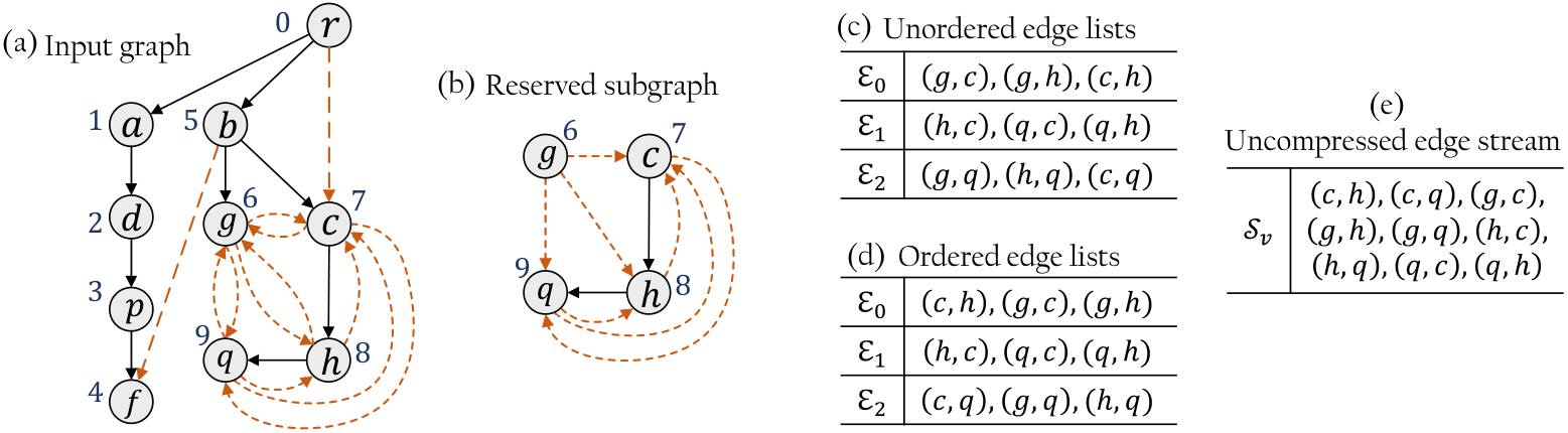
Finally, -index could be obtained by compressing . Here, the compression algorithm used in this paper is [6, 7], which could achieve the best compression rates (about 2-3 bits per link), as far as we know. In order to utilize our -index, at least two attributes should be maintained for each node on , which are and . The former is the offset value [7] of the node in -index. The latter represents the out-degree of node on the graph composed by the edges in -index.
Based on -index, we construct the edge batch by procedure ObtainingEdges-index, as shown in Procedure 4. It is presented for obtaining the edge batch with a given variable on index -index, and for avoiding random disk accesses.
First of all, Lines 1-2 initialize and as an empty edge set and an empty offset list, respectively. , and . A loop, in Lines 3-16, runs until the value of is no smaller than , or the sum of and is larger than , as shown in Line 9. Here, represents the node on whose depth-first order on is equal to , as demonstrated in Line 4. When the sum of an is larger than , as illustrated in Lines 5-7, we load the edges that are related to the offsets in sequentially to reduce random disk seek operations. Besides, we reset and to an empty offset list and , respectively. If is not equal to in Line 12, then and (, according to Line 9). At the end of each iteration of this loop, is updated to as shown in Line 15.
6.3 How to update
In the naive EP-DFS, after replacing with the DFS-Tree of the graph composed by and the edge batch (Definition 5.4), the value of parameter is updated by the smaller value of and . Even though the way that the naive EP-DFS updates parameter is correct, the difference between the value of (Definition 5.2) and the updated in the naive EP-DFS is still large. Since our EP-DFS can be terminated only when the value of is no smaller than , we have put in a lot of efforts to further increase the value of , after replacing with . Here, represents the DFS-Tree of the graph composed by and the edge batch (Definiton 6.1).
Our current result (Theorem 6.3) shows that, we could set the value of to the smaller value of and , as defined in Definition 6.2.
Definition 6.2
, iff, (i) , and (ii) , if and , then .
Example 6.3 is an instance of one iteration of EP-DFS.
6.4 Optimization
In order to reduce the iteration times of EP-DFS, an optimization is devised in this part. Its pseudo-code is presented in Lines 10-14 of Algorithm 2. For clarity, notation is used to denote the value of initialized in Line 6 or updated in Line 11. Notation is used to denote the value of before it is updated in Lines 8-9. is a threshold for determining when to restructure -index, which normally will be set to , in Line 10. indicates that the difference between the total depth-first orders of and is small.
RoundI-index. This procedure of EP-DFS is used to restructure with all the edges contained in -index, by the following way. First of all, it loads the edges contained in -index by batches, and each batch contains at most edges. For an edge in this index, is loaded into the main memory, iff, the depth-first order of on is no smaller than and the depth-first order of on is larger than . Second, it executes function Rearrangement after every five invocations of DFS. Assuming the input spanning tree is in the form of and the output spanning tree is in the form of , then RoundI updates to .
RoundIReduction-index. This procedure is similar to procedure RoundI, which uses edges in -index to restructure , and updates to as discussed above. In addition to that, it also restructures -index with the way of Procedure 3. To be specific, it scans -index sequentially. For each edge contained in -index, it discards if or , since cannot be a forward cross edge as classified by in the following iterations of EP-DFS. The rest of the edges, which are not discarded, are processed by batches: . For an edge batch , is replaced by the DFS-Tree of the graph composed by and . Then, is ordered in the same way that is ordered in Procedure 3, an example of which is shown in Example 6.2. After all the edge bathes are processed, an edge stream is obtained by merging all the ordered edge batches (lists), with external sort. Then, -index is replaced by the compressed .
6.5 Discussion and Implementation details
Compared with traditional algorithms (Section 3), EP-DFS requires simpler CPU calculation, fewer random disk accesses and lower memory space consumption. The reason is as follows. Firstly, EP-DFS prunes the edges of the input graph efficiently, and only based on the total depth-first order of the nodes on . Secondly, EP-DFS accesses the input disk-resident graph only sequentially; EP-DFS accesses the edges in -index either sequentially or ObtainingEdges. Third, EP-DFS only needs to hold edges of in the main memory, and keeps attributes for each node on , i.e. its depth-first order, and .
Our implementation method for EP-DFS is presented below, which could protect it from being affected by the garbage collection mechanism of the implementation language, e.g. C# and java. We assume each node of the input graph could be represented by a -bit integer. Then, an integer array of length is used for maintaining the node list of . And an integer array of length is used for maintaining edges of , where a half is related to while the others correspond to . Plus, an integer array of length is used for maintaining node attributes. Since we assume that each node could be represented as a -bit integer, it is obvious that and can be represented as a -bit integer. The reason why can also be denoted as a -bit integer is discussed in [6].
The in-memory spanning tree of and one edge batch are maintained in the main memory by arrays and . The elements in are organized as one-way linkedlists. They may represent (i) the unused memory space, (ii) the out-neighborhoods of nodes on , and (iii) a stack discussed later. We let to denote the th element of and let to denote the th element of . Assuming , and node , and are the th node, the th node and the th node of , respectively. Then, (i) represents the rightmost child of is , and (ii) if , then is the left brother of . Thus, every two integers of are used to represent an edge , and each integer of is used to denote the index of an edge in whose head is the rightmost child of its tail. To be more specific, an example of how these two arrays work and in EP-DFS is given in Example 6.4.
Example 6.4
Supposing of Figure 4 is the input graph. The nodes in are mapped into integers . An array of length is initialized, and an array of length is also initialized. The initialized arrays are in from (1) of Table 2. Then, firstly, we load the spanning , as shown in Figure 4(a), into the main memory, when these two arrays are in form (2) of Table 2. Secondly, we add an edge batch as shown in Figure 4(a), when these two arrays are in form (3) of Table 2. Secondly, when we execute an in-memory DFS algorithm to replace with the DFS-Tree (i.e. shown in Figure 4(d)) of the graph composed by and edge batch , the two arrays are in from (4) of Table 2.
| (1) | Description | After initialization | ||||||||||||||||||||
| Index | r | a | b | c | d | f | g | h | p | q | Empty space Index | |||||||||||
| Elements | - | - | - | - | - | - | - | - | - | - | 19 | |||||||||||
| Index/2 | 0 | 1 | 2 | 3 | 4 | 5 | 6 | 7 | 8 | 9 | 10 | 11 | 12 | 13 | 14 | 15 | 16 | 17 | 18 | 19 | ||
| Elements | - | 0 | 1 | 2 | 3 | 4 | 5 | 6 | 7 | 8 | 9 | 10 | 11 | 12 | 13 | 14 | 15 | 16 | 17 | 18 | ||
| - | - | - | - | - | - | - | - | - | - | - | - | - | - | - | - | - | - | - | - | |||
| (2) | Description | When is maintained in the main memory | ||||||||||||||||||||
| Index | r | a | b | c | d | f | g | h | p | q | Empty space Index | |||||||||||
| Elements | 17 | 16 | 14 | 13 | 12 | - | - | 11 | - | - | 10 | |||||||||||
| Index/2 | 0 | 1 | 2 | 3 | 4 | 5 | 6 | 7 | 8 | 9 | 10 | 11 | 12 | 13 | 14 | 15 | 16 | 17 | 18 | 19 | ||
| Elements | - | 0 | 1 | 2 | 3 | 4 | 5 | 6 | 7 | 8 | 9 | - | - | - | 15 | - | - | 18 | 19 | - | ||
| - | - | - | - | - | - | - | - | - | - | - | q | p | h | g | f | d | c | b | a | |||
| (3) | Description | When and an edge batch are maintained in memory | ||||||||||||||||||||
| Index | r | a | b | c | d | f | g | h | p | q | Empty space Index | |||||||||||
| Elements | 17 | 16 | 9 | 13 | 12 | - | 8 | 11 | 10 | - | 7 | |||||||||||
| Index/2 | 0 | 1 | 2 | 3 | 4 | 5 | 6 | 7 | 8 | 9 | 10 | 11 | 12 | 13 | 14 | 15 | 16 | 17 | 18 | 19 | ||
| Elements | - | 0 | 1 | 2 | 3 | 4 | 5 | 6 | - | 14 | - | - | - | - | 15 | - | - | 18 | 19 | - | ||
| - | - | - | - | - | - | - | - | q | c | f | q | p | h | g | f | d | c | b | a | |||
| (4) | Description | When is replaced to the DFS-Tree of the graph composed by and | ||||||||||||||||||||
| Index | r | a | b | c | d | f | g | h | p | q | Empty space Index | |||||||||||
| Elements | 18 | 16 | 9 | 13 | 12 | - | 8 | - | 10 | - | 17 | |||||||||||
| Index/2 | 0 | 1 | 2 | 3 | 4 | 5 | 6 | 7 | 8 | 9 | 10 | 11 | 12 | 13 | 14 | 15 | 16 | 17 | 18 | 19 | ||
| Elements | - | 0 | 1 | 2 | 3 | 4 | 5 | 6 | - | 14 | - | 15 | - | - | - | 7 | - | 11 | 19 | - | ||
| - | - | - | - | - | - | - | - | q | c | f | - | p | h | g | - | d | - | b | a | |||
One advantage, as mentioned above, of this implementation method is that it could protect EP-DFS from being affected by implementation languages, because once initialized, the above arrays will be used until the end of the algorithms. Moreover, based on this implementation method, EP-DFS does not have to maintain an external stack when it needs to replace . Instead, as (i) a stack is also a one-way linkedlist, and (ii) when a node is added into the stack, there must be an edge removed from the main memory, the stack is also maintained by as a one-way linkedlist as we manage all the empty space of . For each node in , to record the most recent node visited before where belongs to , we use the in-memory attribute space of the depth-first orders. That is because, we only need to preserve the order among a very small subset of to update , whose depth-first orders are in the range of , in order to update which is no more than . There are two ways to preserve that order. First, storing them directly on disk. Second, there is no additional disk access required when , where (i) represents the number of the nodes whose depth-first orders on are smaller than ; (ii) represents the number of the nodes whose depth-first orders on are in the range of . The reason is discussed below. As when a node of has a depth-first order on which is no larger than , the edges whose tails are are no need to be loaded into the main memory in EP-DFS, so that it is no need to maintain attributes and . Of course, besides all the arrays mentioned above ( and ), an integer array of length is required for recording whether a node is marked as visited or not, when has more than nodes; otherwise, we will use the highest bit of each element in for recording that.
Furthermore, there are also two benefits of our implementation method. First, procedure Rearrangement is not related to any input or output I/Os. One reason is that is stored in the main memory, where represents the input spanning tree that needs to be rearranged. Procedure Rearrangement rearranges all the out-neighborhoods of the nodes on only based on their weights, as discussed in Section 6.1. Another reason is that, no external space is used to store the weights of the nodes on . In fact, we use to maintain the node weights in procedure Rearrangement. As a node in EP-DFS and its weight are represented by integers, we denote as a directed edge, and store it in by letting to be the rightmost child of in . At the end of procedure Rearrangement, all the edges could be easily and efficiently removed from . Second, it gives EP-DFS a chance to avoid the operation of sorting edge batches in procedure Indexing, without additional memory space requirement. For clarity, when the edge sorting operation required in procedure Indexing is utilized, the main memory only maintains a spanning tree for , and no in-memory DFS algorithm is used in procedure Indexing. Each time it gets a set of edges which is a subset of and contains at most edges. EP-DFS could use to maintain all the elements of the edges of , by storing all the elements of and on disk temporarily and reinitializing these two arrays. Each time at most edges can be loaded into the main memory since in this implementation only has the ability of storing edges. It is worth noting that, after edges are loaded into the main memory, these edges could be immediately output on disk, because we already the out-neighbors of each node on the graph composed by the edges in .
This paper does not present the asymptotic upper bounds for the time and I/O consumption of EP-DFS. Because it is too complicated and deserves another paper, which will be our future work. Given the size of the available memory space, the I/O and CPU costs of EP-DFS are related to (1) the initialized value of parameter , in Line 2 of Algorithm 2; (2) the total iteration times of the loop in Lines 5-16 of Algorithm 2; (3) the number of the edges pruned from -index after executing procedure RoundIReduction. Since the distribution of the edges and nodes in is unknown, and the order of stored on disk is also unknown, it is hard to estimate the initialized value of parameter and the number of the edges contained in -index in Line 4. The number of the edges that contained in the index affects the total iteration times of the loop in Lines 5-16 of Algorithm 2. Also, if some edges are pruned from -index by procedure RoundIReduction, then the total iteration times of such loop will also be affected.
Our current results are shown below, which is under one assumption that the edges of are evenly distributed on disk. Supposing is the block size, is the value of parameter returned by Procedure 1, and . First of all, the I/O consumption of Procedure 1 is since it has to sequentially loads into the main memory twice. The time consumption of Procedure 1 is , because (i) the in-memory spanning tree replacing operation scans at most edges; (ii) Procedure 2 requires time, which is discussed in the followings; (iii) each loop of Procedure 1 runs times. Assuming the nodes in are , and in one invocation Procedure 2, each node () of has out-neighbors on . Thus, the time consumption of Procedure 2 is . Secondly, Procedure 3 requires space on disk, if the edges are evenly distributed in . That is because, when the edges are evenly distributed in , the maximum number of the edges in -index is . Thus, when the edges are evenly distributed in , the external space required by -index is at most bits, as discussed in Section 6.2. The time consumption of Procedure 3 includes (i) , the time cost of scanning all the edges in , (ii) , the time cost of sorting the edges in (Line 7, Procedure 3), (iii) , the time cost of storing on disk and accessing from disk, (iv) , the time cost of merging all the ordered edge lists as demonstrated in Line 13 and (v) , the time cost of compressing . Hence, the time cost of Procedure 3 is . Thirdly, the time and I/O costs of Procedure 4 are obvious which are and , respectively. Then, according to the above discussions, the time and I/O costs of function RoundI are and , respectively. The time and I/O costs of function RoundIReduction are and , respectively.
6.6 Correctness analysis
In this section, we present the correctness analysis for Algorithm 1 and Algorithm 2. Assuming Min represents the smaller value of and .
Theorem 6.1
, where (i) is divided into a series of edge batches , where and if , then ; (ii) , represents the DFS-Tree of the graph composed by and , assuming is in the form of .
Proof 6.1
According to Definition 5.1 and Definition 5.2, the statement is correct, iff, the following statement is correct: “For any edge in , if the tail of has a depth-first order that is smaller than , then is not a forward cross edge of as classified by .” Without loss of generality, we assume that (1) an edge ; (2) . Thus, based on (1), is not a forward cross edge as classified by , since belongs to batch and is the DFS-Tree of the graph composed by and . Besides, based on (2) and Definition 5.1, , that is, the depth-first order of is unchanged during the whole process.
Hence, for all the nodes , if , then , because of . Since is not a forward cross edge as classified by , it could be a tree edge, a forward edge, a backward edge, and a backward cross edge as classified by . For one thing, when is a tree/forward edge as classified by , that is and is one of the ancestors of on . To be a forward cross edge as classified by , node should be removed from the subtree rooted at , since a forward cross edge has a tail and a head which are from diffident subtrees of , as discussed in Definition 2.4. That is the depth-first order of should be increased to be larger than the that of the right brother of , which is impossible according to Stipulation 2.1. For another, when is a backward (cross) edge as classified by . In this case should still be a backward edge as classified by any tree among , since the depth-first order of is smaller than that of during the whole process as discussed above.
Theorem 6.2
For a node in , when we compute the weight of , the weights of the children of all have been computed, in procedure Rearrangement.
Proof 6.2
Theorem 6.3
, if , where is the DFS-Tree of the graph composed by and .
Proof 6.3
Theorem 6.4 states the correctness of our optimization algorithm.
Theorem 6.4
If procedure RoundI or procedure RoundIReduction returns and , then .
Proof 6.4
It can be derived from Theorem 6.3 that: “In the th iteration of EP-DFS, , if and , then cannot be a forward cross edge as classified by in the th () iteration of in EP-DFS”. Thus, the correctness of this statement could be proved based on Theorem 6.1, which is discussed below. For one thing, our -index is obtained after the value of is given. Moreover, in the computation process of -index, , is contained in -index, iff, and . For another, in procedure RoundI or procedure RoundIReduction, an edge is discarded, iff, and .
The termination proof and the correctness proof of EP-DFS are given in Theorem 6.6.
Theorem 6.6
Algorithm 2 can be finally terminated, and returns as a DFS-Tree of .
Proof 6.5
Termination proof. The loop in Lines 5-16 of Algorithm 2 ends when . In other words, Algorithm 2 can be terminated iff the value of could exceed , which can be proved based on the following two points. One is, based on the discussions on Section 2, there exists an edge batch , where . Another is, according to Theorem 6.3, the value of must increase in each iteration of the loop (Lines 5-16 of Algorithm 2).
7 Experimental Evaluation
In this section, we evaluate the performance of the proposed algorithm, EP-DFS, against the EB-DFS and DC-DFS algorithms, on both synthetic and real graphs. Specifically, we are interested in the efficiency and the number of I/Os for each algorithm on each graph, where we measure the former by the running time, and the latter by the total size of disk accesses. Besides, with the assumption that each input graph are stored on disk in the form of edge list, we are also interested on the effects of the different disk edge storage methods, i.e. random list (default storage method) and adjacency list (the directed edges with the same tail are continuous stored in disk.). Our experiments run on a machine with the intel i7-9700 CPU, 64 GB RAM and 1TB disk space. All the algorithms in our experiments are implemented by Java. Note that, we limit each experiment within eight hours, and we restrict that at most edges could be hold in the main memory, as discussed in our problem statement (Section 2).
Datasets. We utilize various large-scale datasets including both real and synthetic graphs. The storage method for all utilized graphs is default to random list on disk.
The real datasets are presented in Table 3, which include one relatively small graph, two social networks, and several large crawls or massive networks from different domains33 3 https://github.com/google/guava/wiki/InternetDomainNameExplained. cnr-2000 is a relatively small crawl based on the Italian CNR domain. amazon-2008 describes the similarity among the books of Amazon store, which is a symmetric graph. hollywood-2011 is one of the most popular social graphs, in which the nodes are actors, and each edge links two actors appeared in a movie together. eu-2015-host is the host (the maximum number of pages per host is set to 10M) graph of eu-2015, which is a large snapshot of the domains of European Union countries, taken in 2015 by BUbiNG [5] and starting from the site “http://europa.eu/”. uk-2002 is a 2002 crawl of the .uk domain performed by UbiCrawler [4]. gsh-2015-tpd is the graph of top private domains of gsh-2015, which is a large snapshot of the web taken in 2015 by BUbiNG, similar to graph eu-2015 but without any domain restriction. it-2004 is a fairly large crawl of the .it domain. sk-2005 is 2005 crawl of the .sk domain performed by UbiCrawler. All the above utilized datasets can be accessed from the website “http://law.di.unimi.it/datasets.php”.
| Dataset | LCC | EB-DFS | DC-DFS | EP-DFS | |||||||
|---|---|---|---|---|---|---|---|---|---|---|---|
| RT | I/O | RT | I/O | RT | I/O | IS | |||||
| cnr-2000 | |||||||||||
| amazon-2008 | |||||||||||
| hollywood-2011 | - | - | |||||||||
| eu-2015-host | |||||||||||
| uk-2002 | |||||||||||
| gsh-2015-tpd | - | - | - | - | |||||||
| it-2004 | - | - | - | - | |||||||
| sk-2005 | - | - | - | - | |||||||
The synthetic datasets are randomly generated [12], according to Erdös-Rényi (ER) model (default model) and scale-free (SF) model. Firstly, for a dataset in ER model, we randomly and repeatedly generate an edge that and , where the edges in are unique. Then, for the datasets following SF model, the generation method is in the way in [1], where the parameters , and are set to , and , respectively.
Comparison algorithms and implementation details. In literature, many algorithms are proposed for addressing the DFS problem [15]. However, only a few of them could be used on semi-external memory model, since it is non-trivial to solve the DFS problem under the restriction that only a spanning tree of the input graph could be maintained in memory. These algorithms include EE-DFS, EB-DFS, and DC-DFS, as discussed in Section 3. Among these algorithms, EE-DFS is extremely inefficient, because it processes the edges of one by one instead of edge batches. Thus, in this section, we evaluate our EP-DFS against EB-DFS and DC-DFS.
We prefer the most efficient data structures in the limited main memory space (as discussed in Section 2 and Section 6). For example, in EB-DFS, we utilize our rearrangement algorithm. The division technique used in the evaluated DC-DFS algorithm is Divide-TD, as the other division technique is inefficient reported in [20]. In addition, we develop the DC-DFS algorithm based on Tarjan algorithm (fast strongly connected component algorithm) [17] and Farach-Colton and Bender Algorithm (fast LCA algorithm) [2] to ensure the efficiency of DC-DFS algorithm. Note that, in EP-DFS, if Min in Line 10 and Line 12, Algorithm 2, we say , and we set the threshold to by default.
7.1 Exp 1: Performance on real large graphs
We evaluate the semi-external DFS algorithms on eight real graphs. The disk storage method for all the utilized graphs is default to random list. The evaluation results on the real datasets are demonstrated in Table 3, where we also present (external) space (index size, IS) cost for function Indexing (Line 4) of EP-DFS. The indexing or restructuring time of -index in EP-DFS is included in the running time (RT) of EP-DFS.
Table 3 shows that, compared to EB-DFS and DC-DFS, our EP-DFS could achieve a great performance on the complex real datasets. In other words, EP-DFS is an order of magnitude faster than EB-DFS and DC-DFS, on the reported results. Besides, EP-DFS’s I/O consumption is also greatly lower than one-tenth of EB-DFS’s and DC-DFS’s I/O consumption. For example, to obtaining a DFS-Tree of dataset eu-2015-host, EB-DFS costs s and MB I/Os; DC-DFS requires s and MB I/Os; EP-DFS could be accomplished within s and MB I/Os. That is EB-DFS and DC-DFS consume and times as much time as EP-DFS, respectively, and they require and times as much space as EP-DFS, respectively. Note that, the experimental results also reflect that the indexing process of -index is efficient, and the external space that such index requires is considerably small compared to or .
In addition, we test the three algorithms on hollywood-2011, uk-2002 and sk-2005, by randomly selecting edges from such datasets, as demonstrated in Figures 8-10. We vary the number of edges from to , as shown in the x-axes of Figures 8-10. The chosen reason of such datasets against the others is as follows: (i) hollywood-2011 is the dataset with the highest average node degree (), i.e. ; (ii) uk-2002 is a relatively large graph among the given eight real graphs whose largest connected component contains more than half of nodes; (iii) sk-2005 is the graph with the largest scale including a large connected component with about M nodes. Specially, in order to generate a random graph of an input graph that , we scan all the edges in , where, for each edge , is selected independently, and added into with probability. Since the number of the edges in is huge, the size of the generated edge set is , according to the law of large numbers [3].
The experimental results in Figures 8-10 confirm that our EP-DFS outperforms the traditional algorithms on the real large graphs with different structures. Firstly, in Figure 8, the EB-DFS algorithm cannot construct the DFS-Tree when the generation percent exceeds , while, even on entire hollywood-2011 dataset, the cost of EP-DFS is only about s. The reason is that EB-DFS needs to execute function Round many times, when the structure of the input graph goes more complex, according to the discussion about the “chain reaction” in Section 5. Secondly, in Figure 8, the performance of DC-DFS is poor, which consumes more than s for each generated graphs of uk-2002, compared to the performance of EP-DFS, which requires less than s on the entire uk-2002 dataset. Besides, even though the I/O costs of DC-BFS on the , uk-2002 graphs are less than that on the uk-2002 graph, the time costs are nearly the same. That is because the processes of DC-DFS on such datasets are related to random disk I/O accesses, which is discussed in Section 2. Then, in Figure 10, both DC-DFS and EB-DFS are terminated because of the time limitation, when exceeds on the sk-2005 dataset.
7.2 Exp 2: The impact of varying on synthetic graphs
We vary the number of the nodes from to , for the graphs in ER model, and we set the average node degree () to , for each generated graph. All the graphs are stored on disk in the form of random list. The experimental results about the time and I/O consumption of the evaluated algorithms are presented in Figure 10(a) and Figure 10(b), respectively. As the number of nodes grows, the running time and the number of I/Os required by each evaluated algorithm increase. However, among all the algorithms, EP-DFS has the lowest increasing rate, and EB-DFS has the highest increasing rate. The reason is that, when the number of the nodes increases, the size of the entire input graph grows, i.e. from M to M. Since the “chain reaction” exists, restructuring the in-memory spanning tree to a DFS-Tree goes harder, where the invocation times of both function Round and function Reduction-Rearrangement increase in EB-DFS. In contrast, our EP-DFS, after constructing -index, could avoid scanning the entire input graphs. Besides, our EP-DFS greatly reduce the number of the I/Os, which only requires about MB total size of disk accesses.
7.3 Exp 3: The impact of varying on synthetic graphs
We vary the average degree of the nodes from to , for the graphs in ER model, in this part. The node number is default to , and the storage method is random list by default. The experimental results about the time and I/O cost are depicted in Figure 12(a) and Figure 12(b), respectively, which demonstrate that: with the increase of (the average node degree), the numbers of the running time and the disk I/O accesses are increased. Since the chain reaction exists, the number of I/Os required by algorithm EB-DFS is far beyond , and the running time reaches the time limit, i.e. 8 hours, when . Plus, the performance of DC-DFS is acceptable, even though that of DC-DFS is worse than that of EP-DFS which requires less than s and I/Os.
7.4 Exp 4: The impact of different disk storage methods
For the two kinds of disk storage algorithms, we evaluate all the algorithms on the graphs, where the node numbers are set to , and we vary the average node degree from to . All the graphs are synthetic datasets and in the form of ER model. In other words, we restore all the utilized synthetic datasets in Exp 3 in the form of adjacency list. The experimental results on the graphs stored in the form of random list are presented in Figure 12, while that in the form of adjacency list are depicted in Figure 12. Such results show that there is an increase trend when the number of increases, no matter what disk storage method is. However, the performances of both the two traditional algorithms are worse when the input graphs are stored in the form of adjacency list, while, the performance of EP-DFS is slightly better. Furthermore, both EB-DFS and DC-DFS reach the time limit in the experiments depicted in Figure 12. Such experimental results indicate that (i) the different graph storage method changes the orders of the edges on disk, which affects the process of restructuring an in-memory spanning tree to a DFS-Tree; (ii) compared to the traditional algorithms, our EP-DFS algorithm is more adaptable to the different disk-resident graph storage methods.
7.5 Exp 5: The impact of different graph structures
In this part, we evaluate all the three semi-external DFS algorithms on both ER and SF graphs. Each group of the experiments runs on the graphs with fixed node number, i.e. , in which we vary the average node degree in the range of . Plus, the disk storage method of each graph is default to random list. The experimental results of the running time and the number of disk I/O accesses on ER graphs are depicted in Figure 12(a) and Figure 12(b), respectively, and that on SF graphs are demonstrated in Figure 14(a) and Figure 14(b), respectively. The performances of the evaluated algorithms on the SF graphs are better than that on the ER graphs. However, the time and I/O consumption of DC-DFS on certain SF graphs are higher than that of the other two algorithms. The reason is that, the division process of DC-DFS is hard on the SF graphs generated in the way of [1], in which, the more links that a node is connected to, the higher the probability that it adds a new edge related to .
7.6 Exp 6: The impact of fixing on synthetic graphs
Since the performance of the semi-external DFS algorithms is related to the scales of the input graphs, we are interested in the performance of the three algorithms on the synthetic graphs with fixed edge number. Specifically, in this part, we set to for each generated graph, and vary average degree from to , as depicted in Figure 14. The disk storage method is default to random list. The node numbers of the graphs are M, M, M, M and M, respectively. The experimental results of the running time and the number of required I/Os are demonstrated in Figure 14(a) and Figure 14(b), respectively. According to the depicted results, the performance of EB-DFS algorithm goes worse, when the average degree of input graph increases. Especially, when and , the EB-DFS reaches the time limit. Because, with the fixed size of , the larger number of , the more complex the graph structure is, which causes numerous chain reactions in the restructuring process. In contrast, EP-DFS and DC-DFS could address the given input graphs with higher efficiency and less I/Os, according to Figure 14, with the increase of the average degree.
8 Conclusion
This paper is a comprehensive study of the DFS problem on semi-external environment, where the entire graph cannot be hold in the main memory. This problem is widely utilized in many applications. Assuming that at least a spanning tree can be hold in the main memory, semi-external DFS algorithms restructure into a DFS-Tree of gradually. This paper discusses the main challenge of the non-trivial restructuring process with theoretical analysis, i.e. the “chain reaction”, which causes the traditional algorithms to be inefficient. Then, based on the discussion, we devise a novel semi-external DFS algorithm, named EP-DFS, with a lightweight index -index. The experimental evaluation on both synthetic and real large datasets confirms that our EP-DFS algorithm significantly outperforms traditional algorithms. Our future work is to present the asymptotic upper bounds of the time and I/O costs of EP-DFS. It is interesting but intricate, since the performance of EP-DFS is affected by many interrelated factors as demonstrated in this paper.
Acknowledgments
This paper was partially supported by NSFC grant 61602129.
References
- [1] R. Albert and A.-L. Barabási. Topology of evolving networks: Local events and universality. Phys. Rev. Lett., 85:5234–5237, Dec 2000.
- [2] M. A. Bender, M. Farach-Colton, G. Pemmasani, S. Skiena, and P. Sumazin. Lowest common ancestors in trees and directed acyclic graphs. J. Algorithms, 57(2):75–94, 2005.
- [3] J. K. Blitzstein and J. Hwang. Introduction to Probability. Chapman and Hall/CRC, 2014.
- [4] P. Boldi, B. Codenotti, M. Santini, and S. Vigna. Ubicrawler: A scalable fully distributed web crawler. Software: Practice & Experience, 34(8):711–726, 2004.
- [5] P. Boldi, A. Marino, M. Santini, and S. Vigna. BUbiNG: Massive crawling for the masses. In Proceedings of the Companion Publication of the 23rd International Conference on World Wide Web, pages 227–228. International World Wide Web Conferences Steering Committee, 2014.
- [6] P. Boldi and S. Vigna. The WebGraph framework I: Compression techniques. In Proc. of the Thirteenth International World Wide Web Conference (WWW 2004), pages 595–601, Manhattan, USA, 2004. ACM Press.
- [7] P. Boldi and S. Vigna. The webgraph framework II: codes for the world-wide web. In 2004 Data Compression Conference (DCC 2004), 23-25 March 2004, Snowbird, UT, USA, page 528, 2004.
- [8] K. Bollacker, R. Cook, and P. Tufts. Freebase: A shared database of structured general human knowledge. In Proc. 22Nd National Conf. Artificial Intelligence - Volume 2, pages 1962–1963, 2007.
- [9] R. E. Bryant and D. R. O’Hallaron. Computer Systems: A Programmer’s Perspective. Pearson, 3rd edition, 2015.
- [10] A. L. Buchsbaum, M. H. Goldwasser, S. Venkatasubramanian, and J. R. Westbrook. On external memory graph traversal. In Proceedings of the Eleventh Annual ACM-SIAM Symposium on Discrete Algorithms, January 9-11, 2000, San Francisco, CA, USA, pages 859–860, 2000.
- [11] T. H. Cormen, C. E. Leiserson, R. L. Rivest, and C. Stein. Introduction to Algorithms, 3rd Edition. MIT Press, 2009.
- [12] M. Drobyshevskiy and D. Turdakov. Random graph modeling: A survey of the concepts. ACM Comput. Surv., 52(6):131:1–131:36, 2020.
- [13] S. Durocher and R. Singh. A simple linear-space data structure for constant-time range minimum query. Theoretical Computer Science, 770:51 – 61, 2019.
- [14] R. Jin, H. Hong, H. Wang, N. Ruan, and Y. Xiang. Computing label-constraint reachability in graph databases. In Proceedings of the ACM SIGMOD International Conference on Management of Data, SIGMOD 2010, Indianapolis, Indiana, USA, June 6-10, 2010, pages 123–134, 2010.
- [15] R. Sedgewick and K. Wayne. Algorithms (Fourth edition deluxe). Addison-Wesley, 2016.
- [16] J. F. Sibeyn, J. Abello, and U. Meyer. Heuristics for semi-external depth first search on directed graphs. In A. L. Rosenberg and B. M. Maggs, editors, Proceedings of the Fourteenth Annual ACM Symposium on Parallel Algorithms and Architectures, SPAA 2002, Winnipeg, Manitoba, Canada, August 11-13, 2002, pages 282–292. ACM, 2002.
- [17] R. E. Tarjan. Depth-first search and linear graph algorithms. SIAM J. Comput., 1(2):146–160, 1972.
- [18] X. Wan, H. Wang, and J. Li. LKAQ: large-scale knowledge graph approximate query algorithm. Inf. Sci., 505:306–324, 2019.
- [19] Z. Zhang, J. X. Yu, L. Qin, L. Chang, and X. Lin. I/O efficient: computing sccs in massive graphs. In Proceedings of the ACM SIGMOD International Conference on Management of Data, SIGMOD 2013, New York, NY, USA, June 22-27, 2013, pages 181–192, 2013.
- [20] Z. Zhang, J. X. Yu, L. Qin, and Z. Shang. Divide & conquer: I/O efficient depth-first search. In T. K. Sellis, S. B. Davidson, and Z. G. Ives, editors, Proceedings of the 2015 ACM SIGMOD International Conference on Management of Data, Melbourne, Victoria, Australia, May 31 - June 4, 2015, pages 445–458. ACM, 2015.