Embedding Directed Graphs in Potential Fields Using FastMap-D
Abstract
Embedding undirected graphs in a Euclidean space has many computational benefits. FastMap is an efficient embedding algorithm that facilitates a geometric interpretation of problems posed on undirected graphs. However, Euclidean distances are inherently symmetric and, thus, Euclidean embeddings cannot be used for directed graphs. In this paper, we present FastMap-D, an efficient generalization of FastMap to directed graphs. FastMap-D embeds vertices using a potential field to capture the asymmetry between the pairwise distances in directed graphs. FastMap-D learns a potential function to define the potential field using a machine learning module. In experiments on various kinds of directed graphs, we demonstrate the advantage of FastMap-D over other approaches.
Introduction
Graph embeddings have been studied in multiple research communities. For example, in Artificial Intelligence (AI), they are used for shortest path computations [\citeauthoryearCohen et al.2018] and solving multi-agent meeting problems [\citeauthoryearLi et al.2019]. In Knowledge Graphs, they are used for entity resolution [\citeauthoryearBordes et al.2013]; and in Social Network Analysis, they are used for encoding community structures [\citeauthoryearPerozzi, Al-Rfou, and Skiena2014]. In general, graph embeddings are useful because they facilitate geometric interpretations and algebraic manipulations in vector spaces. Such manipulations in turn yield interpretable results in the original problem domain, such as in question-answering systems [\citeauthoryearBordes, Weston, and Usunier2014].
Despite the existence of many graph embedding techniques, there are only a few that work in linear or near-linear time11 1 linear time after ignoring logarithmic factors. FastMap [\citeauthoryearCohen et al.2018, \citeauthoryearLi et al.2019] is a near-linear-time algorithm that embeds undirected graphs in a Euclidean space with a user-specified number of dimensions. The efficiency of FastMap makes it applicable to very large graphs and to dynamic graphs such as traffic networks and marine environments for unmanned surface vehicles.
The resulting Euclidean embedding can be used in a variety of contexts. The -variant of FastMap [\citeauthoryearCohen et al.2018] produces an embedding useful for shortest path computations. Here, the distances between the points corresponding to pairs of vertices are used as heuristic distances between them in the original graph; and this distance function is provably admissible and consistent, thereby enabling A* to produce optimal solutions without re-expansions. The -variant of FastMap [\citeauthoryearLi et al.2019] produces an embedding that is generally useful for geometric interpretations. In the multi-agent meeting problem, for example, the problem is first analytically solved in the Euclidean space and then projected back to the original graph using Locality Sensitive Hashing (LSH) [\citeauthoryearDatar et al.2004].
In general, the properties of the Euclidean space can be leveraged in many ways. For example, a Euclidean space is a metric space in which the triangle inequality holds for distances. In addition, in a Euclidean space, geometric objects, like straight lines, angles and bisectors, are well defined. The ability to conceptualize these objects facilitates visual intuition and can help in the design of efficient algorithms for Euclidean interpretations of graph problems.
Despite the usefulness of Euclidean embeddings, Euclidean distances are inherently symmetric and, thus, cannot be used for directed graphs. Directed graphs arise in many real-world applications where the relations between entities are asymmetric, such as in temporal networks and social networks. In this paper, we present FastMap-D, an efficient generalization of FastMap to directed graphs. FastMap-D embeds vertices using a potential field to capture the asymmetry between the pairwise distances in directed graphs. Like the -variant of FastMap, FastMap-D focuses on minimizing the distortion between pairwise distances in the potential field and the corresponding true distances in the directed graph. FastMap-D therefore provides physical interpretations of problems posed on directed graphs by enabling vector arithmetic in potential fields. It is a back-end algorithm meant to support a number of applications, including question-answering, machine learning and multi-agent tasks on directed graphs.22 2 Shortest path computation is just one more application that requires FastMap-D to also consider the properties of admissibility and consistency if the intended search framework is related to A*.
The difference in potential of two points in a potential field is inherently asymmetric and therefore a good choice for capturing distances in a directed graph. FastMap-D constructs a potential function defining the potential field using a machine learning module. Through experiments conducted on various kinds of directed graphs, we demonstrate the advantage of FastMap-D over other approaches, including those that directly apply machine learning techniques to learning pairwise distances between the vertices.
Related Work
There are a variety of approaches that embed undirected graphs in a Euclidean space. While some approaches simply try to preserve the pairwise distances between vertices in the embedding, other approaches try to meet additional constraints. For example, [\citeauthoryearLinial, London, and Rabinovich1995] surveys several methods for the low-distortion embedding of undirected graphs and their usage in algorithmic applications such as clustering. On the other hand, the Euclidean Heuristic Optimization (EHO) [\citeauthoryearRayner, Bowling, and Sturtevant2011] and the -variant of FastMap [\citeauthoryearCohen et al.2018] meet additional constraints on the pairwise distances in the embedding. In particular, these distances satisfy admissibility and consistency, which are useful for shortest path computations with heuristic search.
Global Network Positioning [\citeauthoryearNg and Zhang2002] first embeds landmarks in a Euclidean space and then uses them for a frame of reference. Like EHO, this algorithm relies on solving Semi-Definite Programs (SDPs) or similar approaches that are prohibitively expensive for large graphs. Big-Bang Simulation (BBS) [\citeauthoryearShavitt and Tankel2004] is a different method that simulates an explosion of particles under a force field derived from the embedding error. Although it does not rely on solving SDPs, it is still prohibitively expensive for large graphs.
Existing works on embedding directed graphs, such as Node2Vec [\citeauthoryearGrover and Leskovec2016], LINE [\citeauthoryearTang et al.2015] and APP [\citeauthoryearZhou et al.2017], focus on preserving the proximity of vertices. First-order proximity refers to the distance between two vertices; second-order proximity is related to the similarity of their one-hop neighboring vertices; third-order proximity is related to the similarity of their two-hop neighboring vertices; and so forth. These proximity-preserving embedding algorithms are based on skip-gram models originally developed in the context of Natural Language Processing [\citeauthoryearMikolov et al.2013]. Before training, they generate samples of vertex neighborhoods via parameterized random walks. To represent asymmetric proximities, these techniques use two points for each vertex, one to represent the vertex as a source and the other to represent it as a destination. They are appropriate for link prediction, node labeling and community detection in social networks [\citeauthoryearGrover and Leskovec2016]. These algorithms differ from our approach in important ways. First, they lose the physical interpretation since they use two points for each vertex in directed graphs. Second, they are semi-supervised algorithms that require labels or data about vertex similarities while our approach is an unsupervised approach that does not require any information other than the given directed graph. Third, our approach has a plug-and-play machine learning module that works well even with the Least Absolute Shrinkage and Selection Operator (LASSO) regression method, in which case it has a strongly polynomial runtime [\citeauthoryearStrutz2010]. HOPE [\citeauthoryearOu et al.2016] is another algorithm that tries to preserve higher-order proximities, but it forgoes the use of random walks in favor of an approximate Singular Value Decomposition (SVD) of the similarity matrix. The top eigenvectors define the embedding space. Since HOPE relies on solving SVDs, it is prohibitively expensive for large graphs.
Background

FastMap [\citeauthoryearFaloutsos and Lin1995] was introduced in the Data Mining community for automatically generating Euclidean embeddings of abstract objects. For example, if we are given objects in the form of long DNA strings, multimedia datasets such as voice excerpts and images or medical datasets such as ECGs or MRIs, there is no geometric space in which these objects can be naturally visualized. However, there is often a well-defined distance function between each pair of objects. For example, the edit distance33 3 The edit distance between two strings is the minimum number of insertions, deletions or substitutions that are needed to transform one to the other. between two DNA strings is well defined although an individual DNA string cannot be conceptualized in geometric space. Clustering techniques, such as the -means algorithm [\citeauthoryearAlpaydin2010], are well studied in Machine Learning but cannot be applied directly to domains with abstract objects because they assume that objects are described as points in geometric space. FastMap revives their applicability by first creating a Euclidean embedding for the abstract objects that approximately preserves the pairwise distances between them.
In the Data Mining community, FastMap gets as input a complete non-negative edge-weighted undirected graph . Each vertex represents an abstract object . Between any two vertices and , there is an edge with weight that corresponds to the symmetric distance between objects and . A Euclidean embedding assigns a -dimensional point to each object . A good Euclidean embedding is one in which the Euclidean distance between any two points and closely approximates .
FastMap creates a Euclidean embedding in linear time by first assuming the existence of a very high dimensional embedding and then carrying out dimensionality reduction to a user-specified number of dimensions. In principle, it works as follows: In the first iteration, it heuristically identifies the farthest pair of objects and in linear time. It does this by initially choosing a random object and then choosing to be the object farthest away from . It then reassigns to be the object farthest away from . Once and are determined, every other object defines a triangle with sides of lengths , and . Figure 1(a) shows this triangle. The sides of the triangle define its entire geometry, and the projection of onto is given by . FastMap sets the first coordinate of , the embedding of object , to . In particular, the first coordinate of is and of is . Computing the first coordinates of all objects takes only linear time since the distance between any two objects and for is never computed.
In the subsequent iterations, the same procedure is followed for computing the remaining coordinates of each object. However, the distance function is adapted for different iterations. For example, for the first iteration, the coordinates of and are and , respectively. Because these coordinates fully explain the true distance between them, from the second iteration onward, the remaining coordinates of and should be identical. Intuitively, this means that the second iteration should mimic the first one on a hyperplane that is perpendicular to . Figure 1(b) explains this intuition. Although the hyperplane is never constructed explicitly, its conceptualization implies that the distance function for the second iteration should be changed to: . Here, and are the projections of and , respectively, onto this hyperplane, and is the new distance function.
FastMap-D
In this section, we present FastMap-D, a generalization of FastMap to directed graphs. We assume that the given directed graph, , is strongly connected, that is, there exists a path from any vertex to any other vertex . While FastMap produces an embedding of the vertices in a Euclidean space for undirected graphs, FastMap-D produces an embedding of the vertices in a potential field for directed graphs. A -dimensional potential field is a function . The potential field is used to capture asymmetric distances that are inherent in directed graphs.
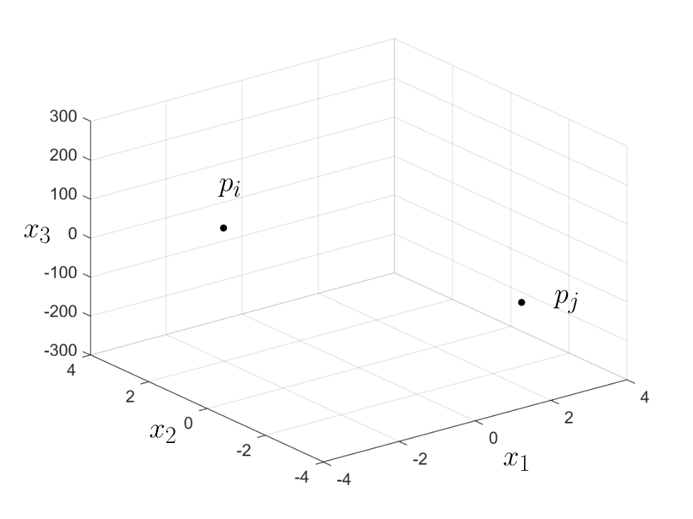
Figure 2 illustrates the difference between the embeddings created by FastMap and FastMap-D. FastMap creates a -dimensional point for each vertex , as shown in Figure 2(a). Here, the Euclidean distance approximates the graph-based distance .
FastMap-D also creates a -dimensional point for each vertex , as shown in Figure 2(b). However, for some -dimensional potential field . The FastMap-D distance , defined to be , approximates . The first term, , approximates the symmetric average distance , and the second term, , approximates the asymmetric correction component .
Algorithm Description
Algorithm 1 presents FastMap-D for directed graphs. The input is a non-negative edge-weighted directed graph along with two user-specified parameters and . is the maximum number of dimensions allowed in the embedding. It bounds the amount of memory needed to store the embedding of any vertex. is the threshold that marks a point of diminishing returns when the distance between the farthest pair of vertices becomes negligible. The output is an embedding (with ) for each vertex .
FastMap-D first embeds all vertices using average distances in a -dimensional Euclidean space (lines 2-25). It then learns a potential function that is used to determine the th coordinate (lines 26-38), which captures asymmetric distances as mentioned above.
Embedding Average Distances:
This phase of the algorithm (lines 2-25) is similar to the regular FastMap procedure that is applicable to undirected graphs. However, the input here is a directed graph, and the distances are asymmetric. Thus, we use the average distances as a symmetric measure derived from the directed graph. All pairwise distances or average distances are never explicitly computed since doing so would be computationally expensive. Instead, we use the function Average-Distance that is invoked only times.
The function Average-Distance (lines 39-43) computes for a given and all . It does this efficiently by computing two shortest path trees rooted at . The first is computed on to yield for all . The second is computed on , which is identical to but with all edges reversed, to yield for all .
In each iteration of (line 4), the farthest pair of vertices () is heuristically chosen in near-linear time (lines 5-14). This pair of vertices is identified with respect to the residual distances for that iteration (line 9).44 4 Note that . The square of the residual distances in iteration , , is the square of the original average distances minus the square of the Euclidean distances already explained by the first coordinates created so far. This is similar to the residual distances used in the -variant of FastMap [\citeauthoryearLi et al.2019]. The farthest pair of vertices, and , are added to pivots, a list of pivots, before the th coordinate for each vertex is computed (lines 16-25) as follows: First, the Average-Distance function is called on and to yield and for all (lines 17-18). Then, the residual distances are computed (line 19), and FastMap’s triangle projection rule is used to compute the th coordinate (lines 23-25).
Learning a Potential Function:
This phase of the algorithm (lines 26-38) constructs a potential function to account for asymmetric distances. The value of is recorded in the last coordinate of the embedding . In this phase, a sampling procedure accompanies a learning procedure to construct . As shown in the pseudocode, can be in the form of a multi-variate polynomial of degree on . It can also be in the form of a Neural Network (NN), as attempted in the next section. Of course, any machine learning algorithm can be used in this phase, but we choose to illustrate the pseudocode of the algorithm using polynomial fitting to facilitate our later discussion. While fitting a multi-variate polynomial can itself be done in many ways, here, we use LASSO to find the unknown coefficients of the multi-variate polynomial. The complexity of LASSO depends on the number of training samples [\citeauthoryearEfron et al.2004].
The sampling procedure uses two qualifying sets and (line 27), and all pairs with and are used as training samples (line 32). The number of training samples is therefore . Different variants of FastMap-D can be created by varying the choices of and . To keep the learning procedure efficient, both and cannot simultaneously be large subsets of . On the other hand, restricting and to significantly smaller subsets can negatively impact the accuracy of the learning procedure. Therefore, FastMap-D chooses and judiciously, sometimes using pivots computed in the first phase of the algorithm.
Consider a multi-variate polynomial of degree having the form , where and for . The number of terms, , in the multi-variate polynomial is given by . We construct to be the vector of unknown coefficients of . is a matrix in which row corresponds to sample . For sample , evaluates to a linear combination of the unknown coefficients and is desired to be equal to the correction factor , which is held in . Therefore, is equal to the coefficient of in .55 5 has unknown coefficients on line 35 and, thus, evaluates to a linear combination of the unknown coefficients. However, on line 38, the unknown coefficients have been determined and, thus, evaluates to a real number.
Like the Ordinary Least Squares (OLS) method, LASSO minimizes in time to determine the unknown coefficients (line 36). However, it uses regularization to address the regularization issues of OLS [\citeauthoryearStrutz2010].
Time Complexity
FastMap-D makes calls to Average-Distance. The time complexity of Average-Distance is . Therefore, the time complexity of the first phase of FastMap-D is . Since LASSO takes time, the overall time complexity of FastMap-D is , which is linear in , near-linear in the size of the graph, linear in the number of training samples and exponential in the degree of . In the next section, we discuss how to keep low. We also keep the degree of to a low constant.
Experiments
In this section, we present experimental results that demonstrate the benefits of FastMap-D. We conduct three kinds of experiments: (1) Comparing the accuracy of the embedding produced by FastMap-D to that of FastMap; (2) Evaluating different combinations of parameter values, specifically, the number of dimensions66 6 in pseudocode of Algorithm 1 and the degree of the potential function ; and (3) Evaluating the effectiveness of NNs trained on the FastMap coordinates of the vertices over NNs trained directly on the grid coordinates of the vertices. All experiments were conducted and evaluated on a 3.4GHz Intel-Xeon CPU with 64GB RAM. All algorithms were implemented in Python.
In our experiments, we also use a few implementation-level enhancements of the pseudocode of Algorithm 1. First, to exercise more control over the number of dimensions , and to experiment with larger values of it, we try to avoid the break condition on line 21. We recognize that, if on line 11, the break condition on line 21 is satisfied. Therefore, we modify line 11 to reassign and randomly and continue the loop without breaking if indeed . We also modify line 21 to set to instead of breaking the loop.77 7 Otherwise, has a very low value, and the division in line 25 leads to numerical instability. Second, to avoid obtuse triangles for the cosine law projection in Figure 1(a), we modify lines 23 and 24 so that and .
Since the machine learning module of FastMap-D is designed to be a plug-and-play component, we implemented it using LASSO as well as an NN method.88 8 Unless specified otherwise, FastMap-D refers to the version with LASSO. For LASSO, we found it beneficial to set to pivots since the pivots can be thought of as critical vertices identified in the first phase of FastMap-D. is set to a randomly chosen subset of vertices such that . For training NNs, however, we generated training samples slightly differently (as described later in that subsection).
Although there exist benchmark instances for directed graphs, none of them come with the assurance of being strongly connected. For this reason, and to allow for a direct comparison with FastMap, the maps in this section are taken from a standard benchmark repository for undirected graphs [\citeauthoryearSturtevant2012], which were also used in [\citeauthoryearCohen et al.2018, \citeauthoryearLi et al.2019]. For each map, we converted every edge into two directed edges in opposite directions to generate a directed version of it. We first created a virtual height for each vertex based on its 2D grid coordinates . The height is assigned according to two possibilities: (a) polynomial function , or (b) exponential function . Then, we set to be if , and otherwise.
To measure distortion, we use the Normalized Root Mean Square Error (NRMSE). We sample random distances between nodes, and compare them against their corresponding embedding distances . To normalize the data coming from graphs of different sizes, the NRMSE is given by where and .
FastMap vs FastMap-D:


Figure 3 shows the NRMSE values of FastMap and FastMap-D for different values of the number of dimensions on four different kinds of maps. The top four panels show the results using the polynomial height function,99 9 Using the polynomial height function for edge weights does not mean that the shortest path distances between vertices follow the same pattern. This is so because the map still has obstacles and the edge weights combine in complex ways to form shortest paths and graph distances. and the bottom four panels show the results using the exponential height function. In all cases, we set the degree of to . Since FastMap works only for undirected graphs, it can only embed the symmetric distances . In other words, FastMap and FastMap-D differ only in the last coordinate that FastMap uses as an additional coordinate and FastMap-D uses as a correction factor to account for asymmetric distances.
We observe that FastMap-D outperforms FastMap on all maps for a sufficiently large number of dimensions . Not only does FastMap-D outperform FastMap on mazes and random maps, but it also significantly outperforms FastMap on structured game maps and real-world city maps such as ‘hrt201n’ and ‘Boston 2_256’. We also note that the FastMap-D NRMSE values often decrease faster than the FastMap NRMSE values for increasing . This shows that FastMap-D utilizes additional dimensions better than FastMap does.
Varying FastMap-D Parameter Values:


Figure 4 shows the effect of and on the NRMSE values of FastMap-D for a representative map. In general, increasing improves the NRMSE values. However, increasing is not always very helpful.
NNs on FastMap Coordinates:
| Instance | Direct NN | FastMap-D (NN) | FastMap-D (LASSO) |
|---|---|---|---|
| Lak503d Poly | 1.238 | 0.048 | 0.042 |
| Lak503d Exp | 0.901 | 0.071 | 0.089 |
| hrt201n Poly | 0.944 | 0.028 | 0.077 |
| hrt201n Exp | 1.239 | 0.083 | 0.271 |
| Boston 2_256 Poly | 0.994 | 0.039 | 0.109 |
| Boston 2_256 Exp | 2.795 | 0.043 | 0.501 |
NNs can learn pairwise distances between the vertices in a grid map. Naively applied, an NN can be trained on the 2D grid coordinates of the source and destination vertices. However, there are several problems with this direct approach. First, it is not applicable to general graphs where vertices do not have coordinates. Second, even for grid maps, the feature set is very small since it is limited to the grid coordinates. Third, it remains oblivious of many parts of the graph even with a large number of training samples since there are a quadratic number of pairs of source and destination vertices.
There are several benefits of using the FastMap coordinates instead of the grid coordinates for training NNs. First, this approach is applicable to general graphs. Second, the feature set is larger and depends on the user-controlled parameter . Third, since the link structure of the graph is summarized in the FastMap coordinates, not too many samples are required. In fact, we simply use randomly selected vertices, compute the shortest path trees rooted at each of them, and draw training samples only from these trees with the source vertex restricted to be the root vertex. This keeps the number of training samples linear in the size of the graph.
Table 1 shows the benefit of training NNs on the FastMap coordinates compared to training them on the grid coordinates. For the same number of training samples, the NRMSE values of FastMap-D with NNs are significantly smaller than those of the direct approach with NNs that uses the grid coordinates. They are also smaller than those of FastMap-D with LASSO.
Conclusions and Future Work
In this paper, we generalized FastMap for undirected graphs to FastMap-D for directed graphs. FastMap-D efficiently embeds the vertices of a given directed graph in a potential field. Unlike a Euclidean embedding, a potential-field embedding can represent asymmetric distances. FastMap-D uses a machine learning module to learn a potential function that defines the potential field. In experiments, we demonstrated the advantage of FastMap-D on various kinds of directed graphs. An important upshot of our approach is that applying machine learning algorithms to the FastMap coordinates of the vertices of a graph is much better than applying them directly to the grid coordinates of the vertices since the FastMap coordinates capture important information of the link structure of the graph - not to mention that the grid coordinates are not even defined for general graphs.
In future work, we will apply FastMap-D to very large directed graphs, such as knowledge graphs, and to intensional graphs, such as in automated planning and plan visualization. The success of FastMap-D exemplifies the benefits of using the FastMap coordinates as features for machine learning algorithms, and we hope to do the same for other graph problems that involve machine learning.
Acknowledgements
The research at Arizona State University was supported by ONR grants N00014-16-1-2892, N00014-18-1-2442, N00014-18-1-2840 and N00014-19-1-2119. The research at the University of Southern California was supported by NSF grants 1724392, 1409987, 1817189, 1837779 and 1935712.
References
- [\citeauthoryearAlpaydin2010] Alpaydin, E. 2010. Introduction to Machine Learning. The MIT Press, 2nd edition.
- [\citeauthoryearBordes et al.2013] Bordes, A.; Usunier, N.; Garcia-Durán, A.; Weston, J.; and Yakhnenko, O. 2013. Translating embeddings for modeling multi-relational data. In Proceedings of the International Conference on Neural Information Processing Systems, 2787–2795.
- [\citeauthoryearBordes, Weston, and Usunier2014] Bordes, A.; Weston, J.; and Usunier, N. 2014. Open question answering with weakly supervised embedding models. In Proceedings of the European Conference on Machine Learning and Principles and Practice of Knowledge Discovery in Databases.
- [\citeauthoryearCohen et al.2018] Cohen, L.; Uras, T.; Jahangiri, S.; Arunasalam, A.; Koenig, S.; and Kumar, T. K. S. 2018. The fastmap algorithm for shortest path computations. In Proceedings of the International Joint Conference on Artificial Intelligence, 1427–1433.
- [\citeauthoryearDatar et al.2004] Datar, M.; Immorlica, N.; Indyk, P.; and Mirrokni, V. S. 2004. Locality-sensitive hashing scheme based on p-stable distributions. In Proceedings of the Annual Symposium on Computational Geometry, 253–262.
- [\citeauthoryearEfron et al.2004] Efron, B.; Hastie, T.; Johnstone, I.; and Tibshirani, R. 2004. Least angle regression. The Annals of Statistics 32(2):407–499.
- [\citeauthoryearFaloutsos and Lin1995] Faloutsos, C., and Lin, K.-I. 1995. Fastmap: A fast algorithm for indexing, data-mining and visualization of traditional and multimedia datasets. In Proceedings of the ACM SIGMOD International Conference on Management of Data.
- [\citeauthoryearGrover and Leskovec2016] Grover, A., and Leskovec, J. 2016. Node2vec: Scalable feature learning for networks. In Proceedings of the ACM SIGKDD International Conference on Knowledge Discovery and Data Mining, 855–864.
- [\citeauthoryearLi et al.2019] Li, J.; Felner, A.; Koenig, S.; and Kumar, T. K. S. 2019. Using fastmap to solve graph problems in a euclidean space. In Proceedings of the International Conference on Automated Planning and Scheduling, 273–278.
- [\citeauthoryearLinial, London, and Rabinovich1995] Linial, N.; London, E.; and Rabinovich, Y. 1995. The geometry of graphs and some of its algorithmic applications. Combinatorica 15(2):215–245.
- [\citeauthoryearMikolov et al.2013] Mikolov, T.; Chen, K.; Corrado, G.; and Dean, J. 2013. Efficient estimation of word representations in vector space. arXiv preprint arXiv:1301.3781.
- [\citeauthoryearNg and Zhang2002] Ng, T. E., and Zhang, H. 2002. Predicting internet network distance with coordinates-based approaches. In Annual Joint Conference of the IEEE Computer and Communications Societies, volume 1, 170–179.
- [\citeauthoryearOu et al.2016] Ou, M.; Cui, P.; Pei, J.; Zhang, Z.; and Zhu, W. 2016. Asymmetric transitivity preserving graph embedding. In Proceedings of the ACM SIGKDD International Conference on Knowledge Discovery and Data Mining, 1105–1114.
- [\citeauthoryearPerozzi, Al-Rfou, and Skiena2014] Perozzi, B.; Al-Rfou, R.; and Skiena, S. 2014. Deepwalk: Online learning of social representations. In Proceedings of the ACM SIGKDD International Conference on Knowledge Discovery and Data Mining, 701–710.
- [\citeauthoryearRayner, Bowling, and Sturtevant2011] Rayner, C.; Bowling, M.; and Sturtevant, N. 2011. Euclidean heuristic optimization. In Proceedings of the AAAI Conference on Artificial Intelligence.
- [\citeauthoryearShavitt and Tankel2004] Shavitt, Y., and Tankel, T. 2004. Big-bang simulation for embedding network distances in euclidean space. IEEE/ACM Transactions on Networking 12(6):993–1006.
- [\citeauthoryearStrutz2010] Strutz, T. 2010. Data Fitting and Uncertainty: A Practical Introduction to Weighted Least Squares and Beyond. Vieweg and Teubner.
- [\citeauthoryearSturtevant2012] Sturtevant, N. 2012. Benchmarks for grid-based pathfinding. IEEE Transactions on Computational Intelligence and AI in Games 4(2):144–148.
- [\citeauthoryearTang et al.2015] Tang, J.; Qu, M.; Wang, M.; Zhang, M.; Yan, J.; and Mei, Q. 2015. Line: Large-scale information network embedding. In Proceedings of the International World Wide Web Conference, 1067–1077.
- [\citeauthoryearZhou et al.2017] Zhou, C.; Liu, Y.; Liu, X.; Liu, Z.; and Gao, J. 2017. Scalable graph embedding for asymmetric proximity. In Proceedings of the AAAI Conference on Artificial Intelligence.