On a nonlinear parabolic problem arising
in the quantum diffusive description
of a degenerate fermion gas
Thanks: This paper has been supported by INDAM (GNFM project “Quantum fluid-dynamics for systems of identical particles: analytical
and numerical study”), by the ANR project number ANR-14-ACHN-0030-01 Kimega and by the bilateral programme “Galileo”, project number G14-34.
Abstract
This article studies, both theoretically and numerically, a nonlinear drift-diffusion equation describing a gas of fermions in the zero-temperature limit. The equation is considered on a bounded domain whose boundary is divided into an “insulating” part, where homogeneous Neumann conditions are imposed, and a “contact” part, where non-homogeneous Dirichlet data are assigned. The existence of stationary solutions for a suitable class of Dirichlet data is proven by assuming a simple domain configuration. The long-time behavior of the time-dependent solution, for more complex domain configurations, is investigated by means of numerical experiments.
keywords
quantum drift-diffusion, fermions, nonlinear parabolic equations, mixed boundary conditionsAMS
35K61, 76Y05, 82D37siapxxxxxxxx–x
1 Introduction
The derivation of quantum fluid equations from quantum kinetic equations [5, 17, 23] is a natural problem in quantum statistical mechanics, in exactly the same way as the derivation of classical fluid equations from Boltzmann equation is a standard topic in classical statistical mechanics [2, 3, 4, 8, 9, 11, 12, 14, 15]. It allows, indeed, to clarify the relationships between two levels of descriptions and to obtain “quantum corrections” to the classical fluid equations, that are difficult (if not impossible) to identify only on the grounds of physical intuition. This is particularly true in the case of a quantum system of identical particles, i.e. obeying either the Bose-Einstein or the Fermi-Dirac statistics [6, 23].
Quantum fluid equations, whose prototype are the Madelung equations [20], are not only important from a theoretical point of view, but they are very interesting also for applications, in particular in semiconductor devices modelling [5, 17, 16, 18]. Indeed, the fluid description of a quantum system has many practical advantages: first of all, it provides a description in terms of macroscopic variables with a direct physical interpretation (such as density, current, temperature); moreover, it allows to model open systems in a very natural way, by imposing suitable semiclassical boundary conditions.
In this article, we study a very specific model, namely the diffusive equation for a degenerate (i.e. at zero absolute temperature) gas of fermions in two space dimensions. The two-dimensional case is rather peculiar, since the third-order “quantum pressure” term, remarkably, vanishes [6, 23]. The resulting diffusive equation have hence the form of a purely semiclassical equation [19], although being (formally) exact up to order . Such equation (after a suitable rescaling of variables) reads as follows [6, 23]:
| (1) |
where is a given potential and , and has therefore the form of a two-dimensional “porous media” equation [24] endowed with a drift term. In this paper we choose to work on Equation (1), not only because of its particularly neat form, but also because the use of two-dimensional models is natural in many instances of semiconductor devices [17, 21].
The mathematical study of Equation (1) has been partially developed in the literature. In particular, existence and uniqueness of a weak solution in the evolutionary case has been proven in [1] and in [13], whereas an analysis of the long-time behaviour has been provided in [10] and [7]. In [1], the time-dependent equation is endowed with mixed homogeneous Neumann and non-homogeneous Dirichlet boundary data; in [10], also the stationary equation is considered, but only in the case of homogeneous Neumann boundary data.
However, a semiconductor device cannot be fully described by imposing only homogeneous Dirichlet boundary conditions. Indeed, for describing real situations, a portion of the boundary (corresponding to metallic contacts) should be described by using non-homogeneous Dirichlet data, whereas other regions of the boundary (corresponding to insulating boundaries) should be supplemented with homogeneous Neumann conditions [17, 21].
The main aim of this article is hence to investigate, both theoretically and numerically, some aspects of Equation (1) by allowing both non-homogeneous Dirichlet boundary data and homogeneous Neumann conditions.
The structure of the article is the following. In the next section we will formulate the mathematical problem and review some basic results on the evolutionary case. Then, in section 3, we will study the stationary case. Particular attention will be given to the situation in which the domain is rectangular and both the data and the potential depend only on one space variable, in which case solutions that depend only on that variable can be considered. A theorem of existence and uniqueness for such solutions, requiring some restrictions on the Dirichlet data, will be proven. Finally, in section 4, we will describe a numerical procedure for studying the initial-boundary value problem and provide some numerical experiments.
2 The mathematical problem
Let be a bounded domain, with a piecewise smooth boundary , and let and be two non-empty subsets of , such that
The gas of fermions in the zero-temperature limit is described by a density function , whose time evolution is governed by the following nonlinear drift-diffusion equation [6]:
| (2) |
Here is a given potential which, for the sake of simplicity, will be assumed to be continuously differentiable. The problem is supplemented with the initial datum
| (3) |
and mixed boundary conditions
| (4) | ||||
where for a.e. , for a.e. and is the outward normal to , at .
Equation , with non-negative mixed Neumann/Dirichlet boundary conditions and has been studied in several works, and its main properties have been analyzed. In particular, existence, uniqueness and preservation of the cone of non-negative functions for problem (2)–(3)–(4) are the specialization to the uncoupled case (without reaction terms) of the results obtained in Ref. [13]. More precisely, by adapting to our case the theorems proven in sections 2 and 3 of Ref. [13], we can state the following:
Theorem 1.
Let , , , and , with non-negative and . Then, there exists a unique non-negative weak solution of the initial-boundary value problem ––, where
Another approach for proving this result consists in transforming Equation (2) into the equation
| (5) |
by means of the transformatiion
| (6) |
i.e.
and then by using the existence and uniqueness theory of Alt and Luckhaus, which studied the class of nonlinear parabolic equations written above, with boundary conditions of type (4), in [1].
In the next section we shall investigate the stationary case and prove (at least for a particular class of initial/boundary conditions) a theorem of existence and uniqueness of the stationary solution. Despite of the general result on the evolutionary equation, we are able to prove a sufficient condition which guarantees the well-posedness of the stationary problem only for a restricted class of “supercritical” Dirichlet data (see Theorem 11).
3 The stationary problem
The study of non-negative stationary solutions of Equation (2), satisfying the prescribed mixed boundary conditions (4), leads to consider the problem
| (7) |
with boundary conditions
| (8) | |||
3.1 A general result in the two-dimensional case
A peculiar feature of the stationary problem is the lack of uniqueness of the stationary solution, as shown in the following proposition.
Proposition 2.
Let us suppose that . If is a non-negative weak solution of the boundary value problem -, then, for every , either or in .
Proof.
This simple result shows that, depending on , the homogeneous stationary problem may have non-unique solution. For example, if with compact support , then both and the function
are non-negative solutions of (7). Moreover, if , then is a strictly positive solution for all constants such that for all (in particular, if is allowed to go to , no positive solution may exist at all).
3.2 Reduction to a one-dimensional problem
We now examine the stationary problem in a particular case, which is basically one-dimensional. Let , let
and let , so that the Dirichlet boundary conditions read as follows:
and the Neumann conditions are imposed on the two other sides of the rectangle.
Moreover, let us assume that
i.e. both the potential and the Dirichlet data only depend on the variable . Then, clearly, is a solution of the stationary problem provided that solves the one-dimensional problem
| (9) | ||||
where we recall that is assumed to be continuously differentiable. We are going to prove that problem (9) has a unique positive solution for positive Dirichlet data, and , subject to suitable restrictions (see Theorem 11).
For the sake of simplicity, from here to the end of this section, we shall denote with the one-dimensional variable ; then, recall that
From (9) we immediately obtain that a constant exists such that
| (10) |
(where the derivatives are now denoted by apices). The case corresponds to all situations in which either or , for some ; in such case, as discussed above, we cannot expect to have uniqueness. Then, we assume and, consequently, we are forced to consider strictly positive Dirichlet data. If , then any regular solution of (10) cannot vanish in and then we can assume to be strictly positive in and write the differential equation in the normal form
| (11) |
Let us first consider the case of constant , for which we have an explicit representation of the solution of the Cauchy problem for the ODE (11). We denote by
respectively, the inverse functions of , and ( is known as the Lambert W-function [22]). It is readily proven that the functions and satisfy the differential equations
| (12) |
Lemma 3.
Let , and . Then, the solution of the Cauchy problem
| (13) |
is given by , where
| (14) |
Moreover, for fixed , we have that is strictly increasing with respect to and , and strictly decreasing with respect to .
Proof.
The fact that satisfies (13) comes straightforwardly from (12). Then we just prove the growth properties with respect to and . Although they could be checked directly on expression (14), it is easier to use the differential equation satisfied by , i.e.
| (15) |
Defining we obtain
| (16) |
and, since for all , we also have
| (17) |
If existed such that in , then from (16) one would obtain
in (where the fact that can be easily checked from (14)) which, together with (17), would give in . Then in , which of course implies that is strictly increasing with respect to .
The proof that is strictly decreasing with respect to can be carried out analogously. ∎
In addition to the properties listed in Lemma 3 let us also note that , as increases from to :
- (i)
increases monotonically from to , if ;
- (ii)
increases monotonically from to the asymptotic value , if and ;
- (iii)
is identically equal to , if and ;
- (iv)
decreases monotonically from to the asymptotic value , if and .
Lemma 3 will allow us to prove properties of the more general differential equation (11) by approximating with piecewise constant functions.
Lemma 4.
Let be a partition of and let be a piecewise constant function, taking the value in the interval , such that uniformly in , as . Let be the solution of the Cauchy problem
| (18) |
with , and let be defined by
(in other words, solves in , taking as initial value in each interval the final value of the preceding interval, starting with in the first interval). Then uniformly in , as .
Proof.
Note that and are continuous solutions of the integral equations,
and
respectively (where, of course, is a piecewise linear approximation of ). Then,
We note that can be decreasing only in the set
Since , we have that
where denotes the maximum positive value of in . Similar considerations hold for (with a lower bound that can be supposed to be independent on ). Then, exists such that for all and, therefore,
Since uniformly in , the thesis follows from Gronwall’s lemma. ∎
Lemma 5.
Let as in the previous lemma and let
Then,
| (19) |
where
Proof.
Let and be as in the previous lemma, and assume, without loss of generality, that for all . In the first interval, , we have , because
as is increasing for decreasing (Lemma 3). Then, in each of the successive intervals we still have , because, a fortiori,
being also increasing with respect to the initial value. Thus in the whole interval . Since, from Lemma 4, uniformly in the inequalities are also true for , which proves our claim. ∎
Note that the result of Lemma 5 implies, in particular, that for all .
Lemma 6.
Let us denote by , with and , the solution of the Cauchy problem . Then, is strictly increasing with respect to , for every fixed .
Proof.
We resort again to the uniformly approximating sequence defined in Lemma 4, that we now denote by in order to stress the dependence on . We can assume, as in Lemma 5, that (independently on ).
From definition (14) it is apparent that is a -function of , piecewise continuous with respect to . However, if we prove that is actually continuous with respect to also at , then has a (positive) lower bound when varies in and, therefore, for any given , and , a constant exist such that
| (20) |
We now prove the continuity of (and of as well) as . For the expression of (which is now seen as a function of and ) is the first one in (14), i.e.
where
By using (12) we easily get
Since as , by applying de l’Hôpital’s theorem we obtain
so that
| (21) |
which, according to (14), proves the continuity of for .
Coming to the -derivative, after straightforward calculations, we have (for )
By using (21) we obtain therefore
which proves the continuity of as .
The continuity of (and ) for is proven in the same way by using the expression of for in (14). This, according to the discussion above, proves (20). We stress the fact that only depends on and , and does not depend on the sequence of the ’s. Then, from the definition of (see Lemma 4) we have that
for all and (small enough), with independent on . Then, passing to the limit for we obtain that is strictly increasing with respect to for every . ∎
Lemma 7.
Referring to Lemma 6 for the notations, we have that converges uniformly to a continuous limit as .
Proof.
It is not difficult to show that
| (22) |
uniformly with respect to , and . Then, still assuming , we obtain that , uniformly with respect to and , where is a continuous, piecewise linear, limit function. Since (seen as a sequence in ) is uniformly Cauchy with respect to and , it is straightforward to prove that is in turn uniformly Cauchy (with respect to ) and, therefore, converges uniformly to a continuous limit . ∎
Definition 8.
To any given data of the Cauchy problem we associate the set of points
by means of the following recursive rule (where ):
- 1.
we start by putting
if , then we put and the procedure ends with , otherwise we proceed to step 2.
- 2.
If we put
if , then the procedure ends with , otherwise we proceed to step 3.
- 3.
If we put
if , then we put and the procedure ends with , otherwise we proceed to step 4.
- 4.
If we put
if , then the procedure ends with , otherwise we increment the index and repeat steps 3 and 4 until we find or for some . (For the sake of simplicity we can assume that changes sign a finite number of times, so that the procedure stops at a finite .)
Finally, we define the continuous function
| (23) |
Lemma 9 (Asymptotic behaviour for ).
Proof.
We divide the proof into three recursive steps.
Step 1. Let be arbitrarily small and let . From Definition 8 we have that exists such that for all . Then, from the obvious inequality
we obtain
which proves that , for all . Since the limit has to be a continuous function (Lemma 7), from the arbitrariness of we also have
Step 2. In the interval we have that (from the previous step) and, by definition, . Then, from Lemma 5
for all .
Step 3. In the subsequent intervals of the form or , we repeat the same proofs of the steps 1 and 2 (respectively), with the only difference that instead of (which implies that Step 1 has to be slightly modified by using a such that for all ). ∎
Note that the limiting process selects one particular solution among the infinitely many solutions of the case , for which we have seen that there is not uniqueness (see section 3.1).
Definition 10.
We define the critical values for the Dirichlet data and as follows:
| (24) |
where we put , and
If a boundary term is greater than the corresponding critical value, then it is said to be supercritical, otherwise it is said to be subcritical.
We can finally prove that the solution of the the Dirichlet problem (9) exists and is unique, provided that the Dirichlet data and are not both subcritical.
Theorem 11.
If , then the Dirichlet problem has a unique, strictly positive,
solution for all .
If , then the Dirichlet problem has a unique, strictly positive,
solution for all .
Proof.
Consider first the case and assume, temporarily, that .
We know that the mapping , obtained by solving the Cauchy problem (18) is strictly monotone. Moreover, from Lemma 5, we have that
since it is easy to see that as , for all and . Moreover, since , from Definition 8 and Lemma 9 we have that
i.e., in particular,
What we have proven so far is that the left-Dirichlet datum can be uniquely linked to any right-Dirichlet datum , by solving the Cauchy problem (18) with a suitable . To go below the threshold we have to consider negative values of . However, the case can always be recast into the case by noticing that, if satisfies , then satisfies
In other words, the forward Cauchy problem with is equivalent to the backward Cauchy problem with . Hence, if we fix the right-Dirichlet datum and take , we can consider the Cauchy problem
| (25) |
that is the backward Cauchy problem for with right-Cauchy datum . What we want to prove is that can be linked to with a suitable choice of . i.e., that exists such that . Since the datum is not necessarily supercritical for problem (25), then in the limit we have in general that tends to the asymptotic solution (with the obvious definition) and, according to the theory we already know, for there are three possibilities:
In the first case (corresponding to supercritical for problem (25) we have (since we have assumed ). In the second case, obviously, and in the third case
(because is supercritical). In each of the three cases, therefore,
and then (owing to the monotonic growth with respect to ), for a suitable . In conclusion, we have shown that the left-Dirichlet datum can be uniquely linked to any right-Dirichlet datum , by solving the Cauchy problem (18) with a suitable .
The proof of the second part of the claim, i.e. the case , is completely equivalent to the proof of the first part since, as we have just shown, it suffices to change into . ∎
4 Numerical simulations
Let and let the square in defined as
We denote moreover
where
and consider the unknowns and .
We now introduce, for , a semi-discrete weak formulation of Equation (2) for the semi-discrete density unknowns and the semi-discrete flux , where is the time step.
Let and . We approximate the weak formulation of Equation (2) by means of the following coupled system
| (26) |
where is the outward normal with respect to starting from a point .
The boundary term (i.e. the integral on in the formulation written above) will be treated in agreement with the different boundary conditions specified for each numerical simulation.
The “positive part” term in the weak formulation (26) is pleonastic at the continuous level, since the solution of the problem is known to be non negative by Theorem 1. At the discrete level, this strategy helps in controlling the non-negativity of the numerical solution.
The numerical experiments aim at showing some peculiar properties of Equation (2) under different choices of the potential and of the boundary conditions, and have been obtained by using the Finite Element Method.
From the semi-discrete formulation, by using quadratic Lagrangian elements on a triangular mesh, we obtain a linear system whose size is given by twice the number of vertices and the number of mid-edges in the triangulation. The system is solved by a multi-frontal Gauss LU factorization.
The simulations are written in FreeFem++. The mesh discretization used in our simulations is composed by 19514 triangles, with 9940 vertices.
4.1 Long-time behavior of the solution in the one-dimensional case
We consider here the boundary conditions
| (27) |
and assume that both the initial datum and the potential only depend on . Then, as already discussed in section 3.2 in the stationary case, the two-dimensional problem reduces to the one-dimensional problem
| (28) | ||||
where the initial datum, , and the (constant) Dirichlet data, and , are positive. In this subsection we report a set of numerical simulations showing that the solution to Equation (28) tends asymptotically to the stationary solution discussed in section 3.2 (see, in particular, Theorem 11). In Figure 1 the spatial profile of the solution along the direction (recall that the solution is homogeneous in the direction ) is shown at different instants of time. This first set of simulations has been performed with the potential
| (29) |
Note that, according to Definition 10, for such potential we have
The initial datum is chosen as a linear function interpolating the values and and the evolution of such datum towards the asymptotic, stationary solution (dotted black curve) is illustrated for different choices of and .
(a)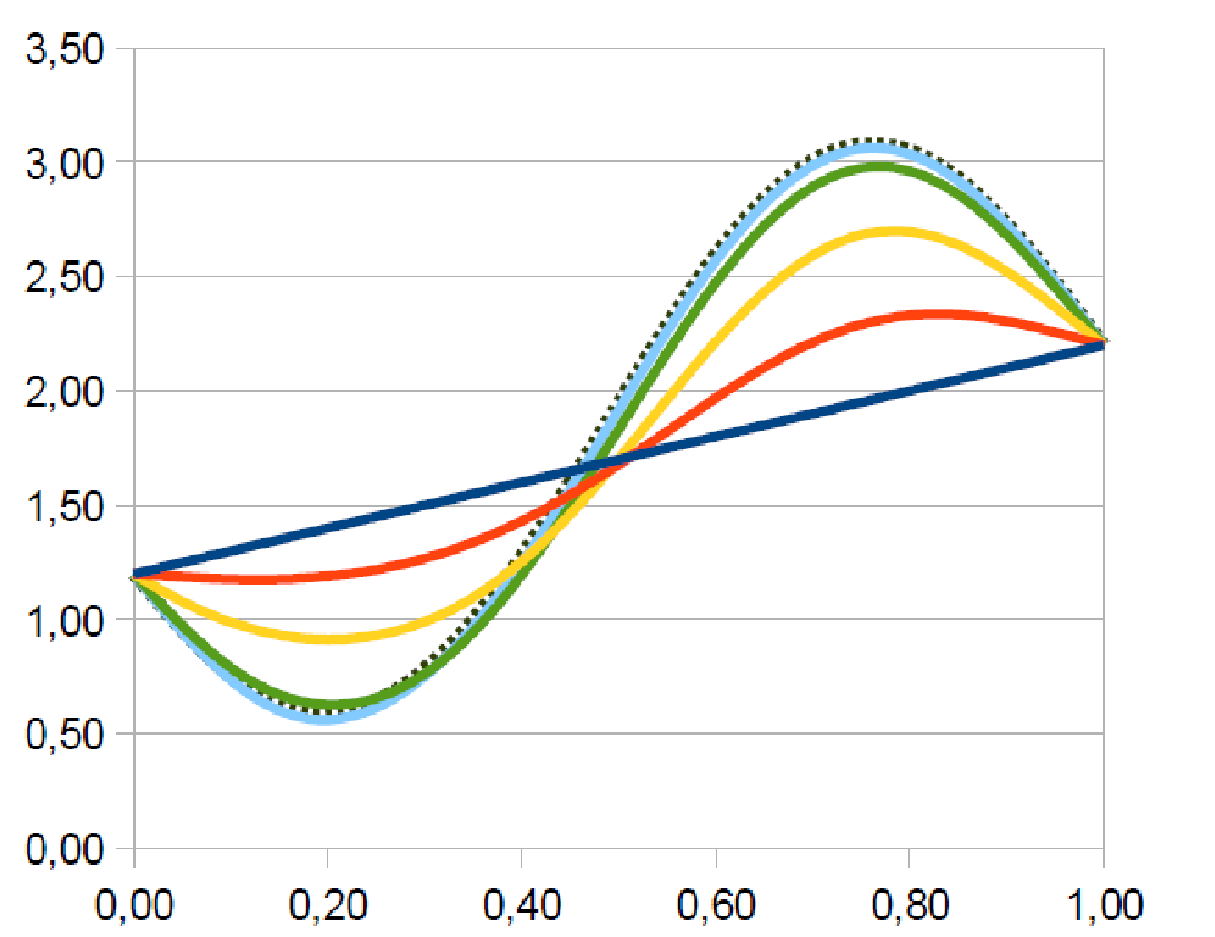 (b)
(b) 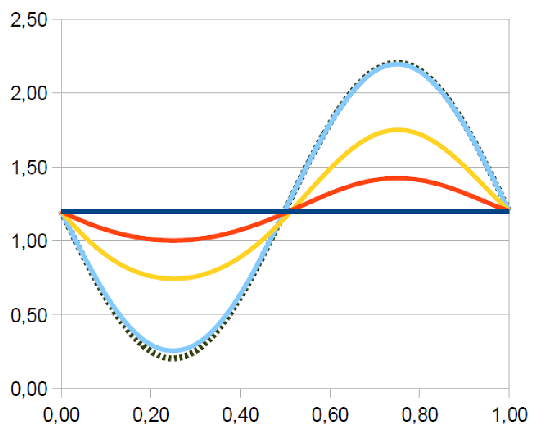
(c) 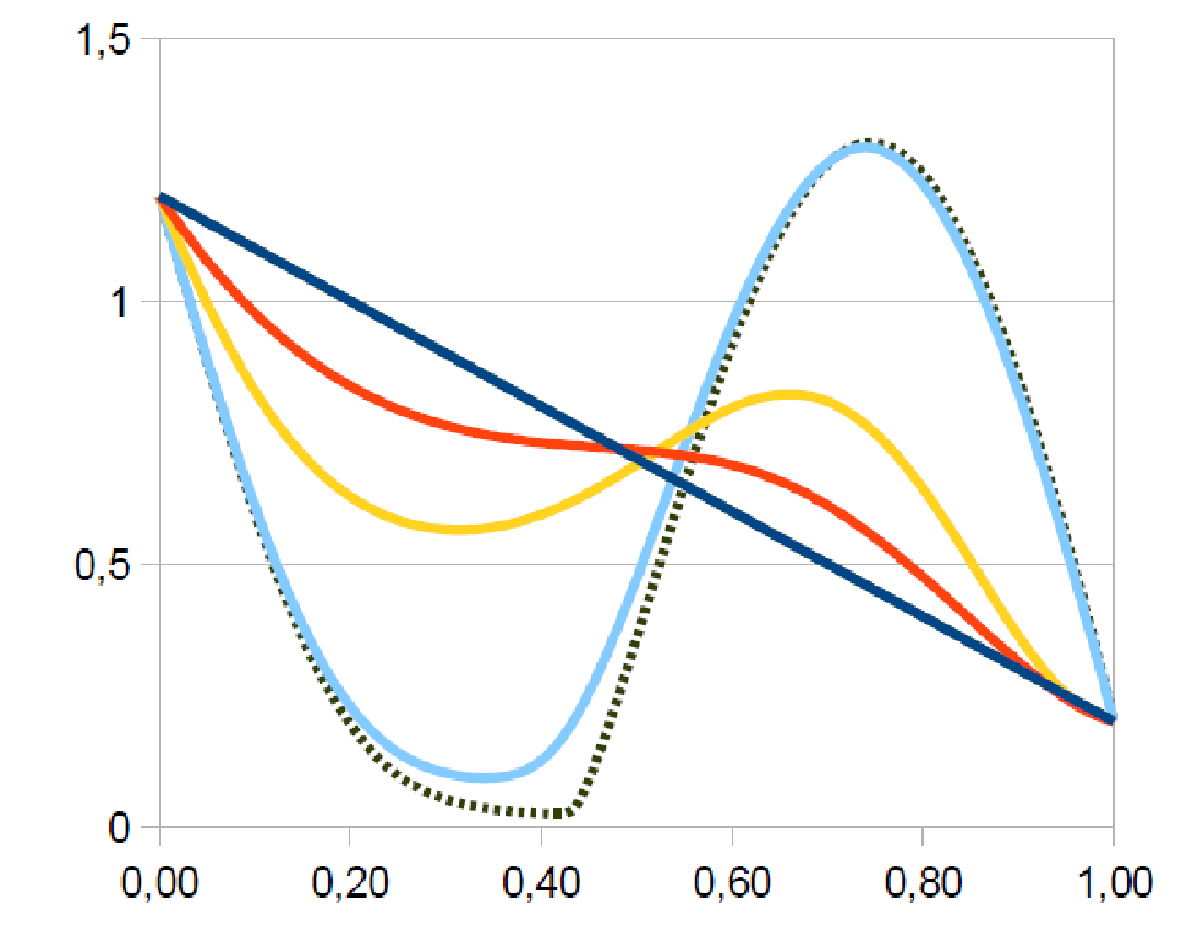 (d)
(d) 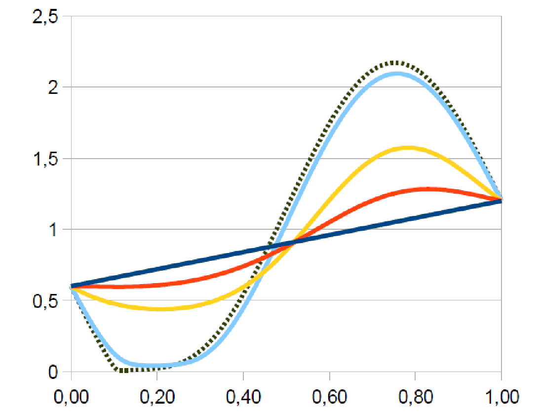
In panels (a), (b), (c) and (d) we have chosen, respectively,
Then, in cases (a) and (b) both data are supercritical while, in case (c), is subcritical and, in case (d), is subcritical. We recall that Theorem 11 guarantees the well-posedness of the stationary problem if at least one of the Dirichlet data is supercritical.
In case (b) since the potential (29) is compatible with equal Dirichlet data, the asymptotic solution is exactly (corresponding to , see definition (23) and Lemma 9). In cases (a) and (d), since , we have that and in case (c), where , we have that (see the proof of Theorem 11 with ). In the three cases (a), (c) and (d), therefore, the asymptotic solution is not (which corresponds to , in the present case where ). Nevertheless, it is interesting to see that the asymptotic curves in Figure 1 tend to have the same character as , i.e. regular in the supercritical cases and piecewise regular in the subcritical cases (however, as long as is finite, the solution is everywhere regular).
4.2 Analysis of the current in the one-dimensional case: monotone potentials
We consider again Equation (2) with the conditions (27) and the following data: and boundary conditions:
For this experiment, we have chosen the potential
Since
the boundary condition in this simulation is supercritical.

In Figure 2, we plot the current versus time that passes through the boundaries (blue dotted line) and (red continuous line), i.e. we visualize the time evolution of
respectively.
We note that, after a transient period, both currents at the extremities of the device tend monotonically to the common value 3.11.
In the second numerical simulation, we have left unchanged the initial and boundary conditions, but we have chosen a different potential, namely
This potential is non-linear, but is still monotone. Here
hence the boundary condition is supercritical.
In Figure 3, we plot the current versus time that passes through the boundaries (blue dotted line) and (red continuous line) respectively.
We note a different behaviour of and with respect to the previous simulation in the transient period before reaching the equilibrium: is still a monotone increasing function, but is no longer monotone. At time (not plotted in Figure 3) the two currents at the extremities of the domain have reached the common asymptotic value 4.01.

4.3 Analysis of the current in the one-dimensional case: a potential barrier
We now consider Equation (2) under the action of the potential
Here the critical values of the problem are
We compare the time evolution of the current at the extremities of the device in two situations. The first one, whose results are plotted in Figure 4, has been obtained with the initial data and the boundary conditions

The second situation, whose result are plotted in Figure 5, has been obtained by imposing the following initial data and the boundary conditions:

The numerical results of Figures 4 and 5 show that the stationary current flowing through the device in the case of a small density gap differ considerably from the one that is obtained in the case of a wide density gap (numerically we get a value which is close to 1.36 in the first case and the value 16.84 in the second). Moreover, in the first case, the convergence speed to the asymptotic state is slower than in the second case.
We have finally computed, for , the asymptotic common value at the ends of the device versus , which is a parameter that controls the gap of the boundary data between the ends and , through the choice of the following initial and boundary conditions:
Both boundary data are supercritical.

The results, plotted in Figure 6, show that the current is zero when and that it is strictly monotone. The profile is parabolic with a good approximation. This simulation has been very time-consuming, since we had to repeat, for each element of the discretization of , a computation in long-time that gives the asymptotic common value of the currents at the ends of the device. The discretization between the values of is , and the final time of each simulation has been . The discrepancies observed between the numerical values of and are, for each value of , beyond the resolution of Figure 6.
4.4 Analysis of the current in a two-dimensional device in a non-symmetric situation
We conclude the description of our simulations with a test-case that is widely used in the literature [21]. Consider the system defined by (2) under the action of the linear potential
In this case, the initial data and boundary conditions are
and
Note that, even though and depend only on the first variable , the problem is genuinely two-dimensional because of the boundary conditions.
a)  b)
b) 
c)  d)
d) 
e)  f)
f) 
In Figure 7, we show the time evolution of the unknown density . At time the system has already reached an almost stationary configuration.

We also show in Figure 8 the time evolution of the -norm of the density . Note that the total mass of the problem is not conserved in time, but has a non-monotone behaviour around the value .
References
- [1] H. W. Alt, and S. Luckhaus, Quasilinear elliptic-parabolic differential equations, Math. Z., 183 (1983), pp. 311–341.
- [2] C. Bardos, F. Golse, and C. D. Levermore, Sur les limites asymptotiques de la théorie cinétique conduisant à la dynamique des fluides incompressibles, C. R. Acad. Sci. Paris Sér. I Math., 309 (1989), pp. 727–732.
- [3] C. Bardos, F. Golse, and C. D. Levermore, Fluid dynamic limits of kinetic equations. I. Formal derivations, J. Stat. Phys., 63 (1991), pp. 323–344.
- [4] C. Bardos, F. Golse, and C. D. Levermore, Fluid dynamic limits of kinetic equations. II. Convergence proofs for the Boltzmann equation, Comm. Pure Appl. Math., 46 (1993), pp. 667–753.
- [5] L. Barletti, G. Frosali, and O. Morandi, Kinetic and hydrodynamic models for multi-band quantum transport in crystals, in Multi-Band Effective Mass Approximations: Advanced Mathematical Models and Numerical Techniques, M. Ehrhardt and T. Koprucki, eds., Springer-Verlag, Berlin, 2014. Chap. 1, pp. 3–56.
- [6] L. Barletti, and C. Cintolesi, Derivation of isothermal quantum fluid equations with Fermi-Dirac and Bose-Einstein statistics. J. Stat. Phys., 148 (2012), pp. 353–386.
- [7] P. Biler, J. Dolbeault, P.A. Markowich, Large time asymptotics of nonlinear drift-diffusion systems with Poisson coupling. The Sixteenth International Conference on Transport Theory, Part II. Transport Theory Statist. Phys. 30 (2001), pp. 521?536.
- [8] L. Boudin, B. Grec, M. Pavić, and F. Salvarani, Diffusion asymptotics of a kinetic model for gaseous mixtures, Kinet. Relat. Models, 6 (2013), pp. 137–157.
- [9] L. Boudin, B. Grec, and F. Salvarani, The Maxwell-Stefan diffusion limit for a kinetic model of mixtures, Acta Appl. Math. (in press).
- [10] J. A. Carrillo, A. Jüngel, P. A. Markowich, G. Toscani, and A. Unterreiter, Entropy dissipation methods for degenerate parabolic problems and generalized Sobolev inequalities, Monatsh. Math., 133 (2001), pp. 1–82.
- [11] C. Cercignani, The Boltzmann equation and its applications, Springer-Verlag, New York, 1988.
- [12] L. Desvillettes, R. Monaco, and F. Salvarani, A kinetic model allowing to obtain the energy law of polytropic gases in the presence of chemical reactions, Eur. J. Mech. B Fluids, 24 (2005), pp. :219–236.
- [13] J. I. Díaz, G. Galiano, A. Jüngel, On a quasilinear degenerate system arising in semiconductors theory. I. Existence and uniqueness of solutions, Nonlinear Anal. Real World Appl. 2 (2001), pp. 305–336.
- [14] F. Golse, and L. Saint-Raymond, The Navier-Stokes limit of the Boltzmann equation for bounded collision kernels, Invent. Math., 155 (2004), pp. 81–161.
- [15] F. Golse, and L.Saint-Raymond, The incompressible Navier-Stokes limit of the Boltzmann equation for hard cutoff potentials, J. Math. Pures Appl. (9), 91 (2009), pp. 508–552.
- [16] A. Jüngel, Quasi-hydrodynamic semiconductor equations, Birkhäuser Verlag, Basel, 2001.
- [17] A. Jüngel, Transport Equations for Semiconductors, Springer-Verlag, Berlin, 2009.
- [18] A. Jüngel, P. Pietra, A discretization scheme for a quasi-hydrodynamic semiconductor model, Math. Models Methods Appl. Sci. 7 (1997), pp. 935–955.
- [19] A. Jüngel, S. Krause, and P. Pietra, Diffusive semiconductor moment equations using Fermi-Dirac statistics, Z. Angew. Math. Phys., 62 (2011), pp. 623–639.
- [20] E. Madelung, Quantentheorie in hydrodynamischer form, Z. Phys., 40 (1926) pp. 322–326.
- [21] P. A. Markowich, C. A. Ringhofer, and C. Schmeiser. Semiconductor equations, Springer-Verlag, Vienna, 1990.
- [22] F. W. J. Olver, D. W. Lozier, R. F. Boisvert, and C. W. Clark, NIST Handbook of Mathematical Functions, Cambridge University Press, Cambridge, 2010.
- [23] M. Trovato and L. Reggiani, Quantum hydrodynamic models from a maximum entropy principle, J. Phys. A, 43 (2010), article 102001.
- [24] J. L. Vázquez, The Porous Medium Equation: Mathematical Theory, Oxford University Press, Oxford, 2007.