A Study on the Baryon Acoustic Oscillation with Topological Data Analysis
Abstract
The scale of the acoustic oscillation of baryons at the baryon-photon decoupling is imprinted on the spatial distribution of galaxies in the Universe, known as the baryon acoustic oscillation (BAO). The BAO provides very useful information in the early Universe. The correlation functions and power spectrum are used as a central tool for the studies on the BAO analysis. In this work, we analyzed the spatial distribution of galaxies with a method from the topological data analysis (TDA), in order to detect and examine the BAO signal in the galaxy distribution. The TDA provides a method to treat various types of "holes" in point set data, by constructing the persistent homology (PH) group from the geometric structure of data points and handling the topological information of the dataset. We can obtain the information on the size, position, and statistical significance of the holes in the data. A particularly strong point of the persistent homology is that it can classify the holes by their spatial dimension, i.e., a 0-dim separation, 1-dim loop, 2-dim shell, etc. We first analyzed the simulation datasets with and without the baryon physics to examine the performance of the PH method. We found that the PH is indeed able to detect the BAO signal among the large-scale structures in the Universe: simulation data with baryon physics present a prominent signal from the BAO, while data without baryon physics does not show this signal. In fact, a systematic method to test the significance of the signal detection from the PH diagram has not been established yet. Then, this examination can be a new reliable method to demonstrate the performance of the PH analysis of the large-scale structure. Then, we applied the PH to a quasar sample at from extended Baryon Oscillation Spectroscopic Survey [1] in Sloan Digital Sky Survey Data Release 14 (SDSS DR14: [2]). We constructed a cubic complete subsample of quasars with a volume of 1 [] and performed the PH. We discovered a characteristic hole (a hollow shell) at a scale . This exactly corresponds to the BAO signature imprinted in the galaxy/quasar distribution. We performed this analysis on a small subsample of 2000 quasars. This clearly demonstrates that the PH analysis is very efficient in finding this type of topological structures even if the sampling is very sparse.
1 Introduction
1.1 Characterizing the Matter Distribution in the Universe
The distribution of matter and galaxies at each epoch of the Universe contains fundamental information on the formation and evolution of the cosmic structures in general [3, 4, 5, e.g.,]. A vast number of sophisticated methods have been proposed to characterize the statistical properties of the fluctuation in the Universe [3, 6, 5, e.g.,]. Among them, the -point correlation functions are the most popular and well-studied methods in the analysis of observational galaxy distribution [3, e.g.,]. Mathematically, the infinite sequence of -point correlation functions are sufficient to specify stochastic random fields [7, 8, e.g.,].
However, in practice, estimating higher-order -point correlations becomes unrealistically difficult, and other approaches that can treat the information of higher-order correlations have been considered. One of the popular methods in cosmology and astrophysics is the so-called "Minkowski Funcionals" [9, 10, 11, e.g.,]. In the applications of the Minkowski Functionals to the Large-Scale Structure, the topology of smoothed density field of galaxy distribution is analyzed by examining the "genus" or number of holes in the density field. Since basically the smoothed random field contains the whole information on the infinitely high-order moments of the field, in principle the Minkowski Functionals can specify the galaxy density field completely. Indeed this method has been applied very extensively to the analysis of the cosmic density field [12, 13, 14, 9, 15, 16, 17, e.g.,], as well as redshift distortion [18, e.g.,], weak lensing cosmology [19, 20, 21, e.g.,], cosmic reionization [22, 23, 24, 25], test of cosmological/gravity theories [26, 27, 28, 29], and the cosmic microwave background (CMB: e.g., [30, 31, 32, 33, 34, 35]).
1.2 From Minkowski Functionals to topological data analysis
In fact, however, the method of Minkowski Functionals, or sometimes called the genus statistics, is a part of more general framework to characterize the properties of a point data set, known in the field of topological data analysis (TDA: e.g., [36, 37, 38]). We briefly overview the method of TDA in the following.
Intuitively, the topological information is characterized by the holes of the object. For the current interest, the object to be analyzed is constructed from -dimensional sphere with radius from discrete data points, i.e., -body particles and/or galaxies (and some other astronomical objects, in general). With the discovery of the 3-dim structure in galaxy distribution [39, e.g.,], an idea of using the geometry (topology) of smoothed density field was proposed to quantify the large scale structure and specify the physics behind it [40, 41, 42, 43, 44, e.g.,]. The basic idea of these early works was an application of random percolation: they set a sphere around each galaxy with an increasing radius, and examine the geometry of connected components in a considered volume. This approach has been developed in relation to the theoretical development of perturbation theory of the cosmic structure [45, 46, 47, 48, 10, 49, 50, e.g.,]. The expectation of the number of genus of the smoothed field as a function of the threshold density is referred to as the genus curve, and it can be expressed analytically with these theories. Since this curve can distinguish between Gaussian and other random fields, it became one of the most popular tools for the analysis of the large-scale structure.
In spite of the great development of the theories of the Minkowski Functionals in cosmology, it was not well recognized that it consists a part of much larger, richer framework studied in the topological data analysis (TDA). The birth of the primitive concept of the TDA dates back to 90’s, but its actual birth was in the new millennium [36, 51, see e.g., ]. The concept directly related to the Minkowski Functionals is the persistent homology (PH) in TDA. Similarly to the random percolation, the PH considers a sphere (solid ball) of radius around each point in a point data set. More sophisticatedly, the PH handles the birth and death of loop structures in various dimensions. This is schematically described in Fig. 1. Consider a set of three points. When the radius is small, we simply have a set of three balls (left of Fig. 1. Then, at some , we have a connected structure, a loop (middle), regarded as the birth of a hole. When becomes larger, the hole in the loop disappears, the death of the hole (right). For general point data set, we trace such a life history of loops with dimension , corresponding to a number of connected components (0-dim), number of loops (1-dim), number of hollow voids (2-dim), , number of -dim holes, respectively. Thus, we can easily imagine that, if we plot the birth and death of these quantities as a function of , this will contain very rich information of the point set. Such a plot is referred to as the persistent diagram (PD) and is the central tool for the PH. Complete definitions and methodology will be thoroughly presented in Section 2.
In spite of the vast number of applications of Minkowski Functionals as mentioned above, extensive applications of the TDA has not been very frequently found in astrophysics and cosmology yet, though it has been gradually known for recent several years. Pranav et al. [52, 53] and Feldgrugge et al. [54] presented a detailed formulation on the stochastic homology of Gaussian and non-Gaussian random fields, gearing at the application to the stochastic field. By the method, they claimed a detection of an anomalous behavior the the CMB fluctuation [55]. Cole and Shiu [56] also developed a method to apply the TDA to the evaluation of the non-Gaussianity of the CMB. Xu et al. [57] applied the PH for a large galaxy data set generated from -body simulation [58] and found 23 voids in the simulation data.
Here, in this work, we introduce the method with the emphasis on the inverse analysis of the detected topological structures, and apply the PH to the signal of the baryon acoustic oscillation.

1.3 The baryon acoustic oscillation
Baryons evolve in a very complicated way via electromagnetic interactions (with radiative heating/cooling, gas pressure, fluid dynamical processes, etc.) A typical example of such a nontrivial phenomenon is the baryon acoustic oscillation (BAO) generated in the matter-radiation fluid in the early Universe [59, 60]. Here we briefly review the BAO and related observables.
Consider a point-like initial perturbation in the primordial matter-photon plasma. In the plasma, the matter and photons are locked into a single fluid. Since the photons are so hot and numerous, the combined fluid has an tremendous pressure with respect to its density. The pressure tries to equalize itself with the surroundings, which results in an expanding spherical sound wave. The sound speed at this early epoch is evaluated by
| (1.1) |
where is the speed of light, and the subscript B and R stand for baryon and radiation, respectively. Equation 1.1 shows that the sound speed before the matter-radiation decoupling can be % of the speed of light at early epoch. Sound horizon (final radius) is obtained by
| (1.2) |
where subscript dec stands for the time of the decoupling between photons and matter. What we actually observe is the superposition of many acoustic waves imprinted on the large-scale structure emerged from the primordial fluctuations. Though the BAO is a baryonic phenomenon by definition, the density enhancement structure of baryons and dark matter becomes the same at the final state [61, 62, e.g.,].
The BAO length scale is constant in comoving coordinates. Then, in principle, we can detect the signal on the galaxy 2-point correlation function. However, since the BAO scale is very large compared to the typical scale of the large-scale structure, we need a very large galaxy sample with dense sampling, since we must measure the signal at such a large scale, where usually the 2-point correlation is very weak. The SDSS is the largest optical photometric and spectroscopic surveys ever existed, covering one-third of the whole sky. Then, the advent of the SDSS finally made it realistic to detect the BAO signal on the 2-point correlation function. Eisenstein et al. [63] first detected the signal around 150 Mpc on the 2-point correlation function. Since then, still this analysis is only possible with SDSS data.
The BAO can be used for various directions of cosmological studies. Then, if a more flexible and easier method for the detection and quantifying the BAO signal exists, it would be desirable. We introduce the PH as such an ideal method for the analysis of BAO. This paper is organized as follows: We introduce the definitions and concepts of the TDA relatively rigorously in Section 2. Especially, we introduce the method of inverse analysis of the PH. Then we examine the performance of the PH as a tool for the studies of BAO by using simulation datasets with and without baryon physics in Section 3. After knowing its power, we apply the PH to quasar data extracted from the extended Baryon Oscillation Spectroscopic Survey (eBOSS) [1] LSS catalog [64] in the SDSS DR14 [2] in Section 4. Section 5 is devoted to our summary and discussion on the result and future prospects of the presented methodology.
In this study, we adopt cosmological parameters , , , and , as constrained by the latest CMB observation by Planck [65] throughout this paper.
2 Topological Data Analysis (TDA)
2.1 Geometric modeling of point cloud data
In the topological data analysis (TDA), we often face a problem to examine topological properties of a finite sequence of points in -dim Euclidean space 11 1 Throughout this paper, , and stand for a set of real number, set of natural number, and non-negative natural number, respectively.. Since is a finite set, a simple application of traditional topological discussion cannot extract any nontrivial information on the features of . Instead, in TDA, a geometric model with a "filtration", , is constructed from the finite point cloud, and topological methods are applied to the model. Here the parameter of the filtration is considered to control the "resolution" or "scale" of the input data. The TDA extract meaningful topological characteristics of the point data by examining the persistent properties along the change of the resolution [36, 66, e.g.,]. We introduce such geometric models that play a fundamental role in the TDA.
2.1.1 Simplex and simplicial complex
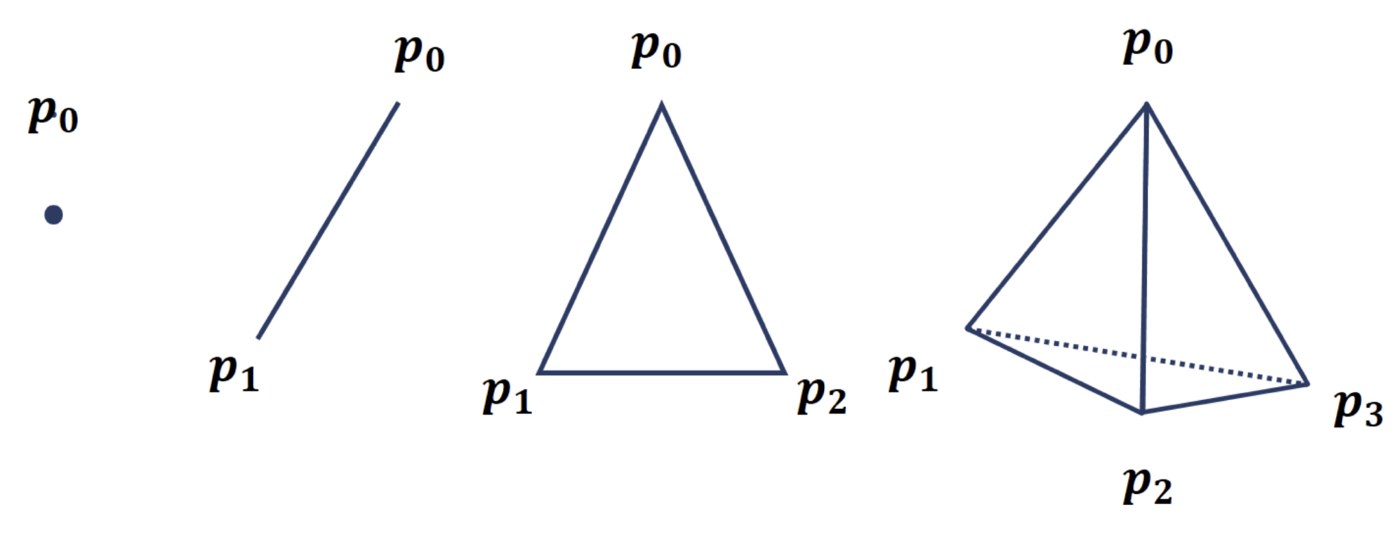
A simplex is a generalization of the notion of a triangle or tetrahedron to arbitrary dimensions. More precisely, it is defined as follows. Points of a finite set in is affinely independent if they are not contained in any affine subspace of dimension less than .
Definition 1 (Simplex)
Suppose a set of points, in -dimensional Euclidean space , arranged to be affinely independent. If we consider vectors , the convex hull that contains these vectors
| (2.1) |
is called -simplex, often denoted as . The dimension of -simplex is defined as .
For example, a -simplex is a point, a -simplex is a line segment, a -simplex is a triangle, and a -simplex is a tetrahedron.
Definition 2 (Face)
Consider a -simplex. The convex hull of any nonempty subset of the points () that define an -simplex is called a face of the simplex.
A face is itself a simplex. The convex hull of a subset of size of the points is defined as -simplex, called an -face of the -simplex. A -face is called the vertex, and a 1-face is the edge. Figure 2 shows the examples of simplices with dimension of 0, 1, 2, and 3. For example, a -simplex in Fig. 2 has seven surfaces , and .
Based on these concepts, we can define the simplicial complex as
Definition 3 (Simplicial complex)
A simplicial complex in is a set of simplices that satisfies the following conditions:
- 1.
Every face of a simplex from is also in .
- 2.
The non-empty intersection of any two simplices is a face of both and .
The maximal dimension of simplices in is called the dimension of the simplicial complex , denoted as . An example of a simplicial complex is presented in Fig. 3.
Definition 4 (Polyhedron)
Consider a union of all the simplices in ,
| (2.2) |
a geometrical shape in is obtained. This shape is referred to as a polyhedron defined by a simplicial complex .

Definition 5 (Abstract simplicial complex)
If a family of non-empty finite subsets of a finite set satisfies the following condition, is an abstract simplicial complex:
- 1.
For every set , ,
- 2.
A subset of , , also belongs to .
Here a subset of , , is called -simplex, whose dimension is defined as . The maximal dimension of simplices in is called the dimension of the abstract simplicial complex, denoted as . As trivially follows from the definition, a simplex consisting an abstract simplicial complex does not need to be in .
A simplicial complex can be treated as an abstract simplicial complex. Inversely, a simplicial complex in can be assigned to an abstract simplicial complex. Consider a point
| (2.3) |
(i.e., only the -th component is and all the others are ) for each element () of an abstract simplicial complex . By these points , we define a simplex for . If we define as a set of all the simplices in obtained as above, satisfies Definition 3. Namely, is a simplicial complex. The polyhedron is called a geometric realization of (e.g., [66]).
2.1.2 Nerve and nerve theorem
As mentioned above, simplicial complices can be seen as purely combinatorial objects, as well as a topological space at the same time. We introduce an important concept "nerve" here.
Definition 6 (Open cover)
An open cover of a set is a collection of open subsets , such that
| (2.4) |
Then, we define a nerve as follows.
Definition 7 (Nerve)
Given a cover of a set , , its nerve is the abstract simplicial complex whose vertex set is and
| (2.5) |
if and only if
| (2.6) |
We denote the nerve of as .
In general, the nerve does not always accurately reflect the topology of , i.e., is not homotopic equivalent to . However, if an intersection of the s is either empty or contractible (see Definition A2), namely a "good cover", the following important theorem holds.
Theorem 1 (The Nerve Theorem)
Let be a finite open cover of a subset such that any intersection of the s is either empty or contractible. Then and the nerve are homotopy equivalent.
2.1.3 Čech complex


Now we relate the filtration and simplicial complex.
Definition 8 (Filtration of simplical complices)
A filtration of a finite simplicial complex is a nested sequence of sub-complices such that
| (2.7) |
where is a simplex of .
We note that a filtration of is just an ordering of the simplices, it may be natural to index the simplices by an increasing sequence of real numbers ,
| (2.8) |
We define the Čech complex as follows.
Definition 9 (Čech complex)
Consider a point set , . Set a sphere with radius around each ,
| (2.9) |
where stands for the Euclid norm. The nerve of the collection of these balls ,
| (2.10) |
is the Čech complex of with radius .
Since a ball satisfies the condition of Theorem 1, we have
| (2.11) |
This means that if we want to examine homotopy invariant characteristics of a set that satisfies the condition of Theorem 1, we can do it equivalently on its nerve . Since the nerve is an abstract simplicial complex, it is much more computer-friendly to calculate such properties. A schematic example of a Čech complex is shown in Fig. 4
The necessary and sufficient condition that -simplex of a Čech complex is
| (2.12) |
Note that this hols for , namely,
| (2.13) |
Thus
| (2.14) |
and therefore, for an increasing sequence , we have an increasing sequence of Čech complices
| (2.15) |
This defines the Čech complex filtration. This enables us to deal not only with the topological information of at a radius but also their transition and persistence with changing .
2.1.4 Voronoi diagrams, Delauney complex and alpha complex

Though the definition of Čech complex is straightforward, computationally it is rather demanding when the data size is large. A more convenient type of complex is desirable for this aspect. We introduce the alpha complex in the following [67, 68]. We first define the Voronoi diagram of a point set.
Definition 10 (Voronoi diagram)
Consider a point set , . A Voronoi diagram can be expressed with Voronoi cells for each point as
| (2.16) | |||
| (2.17) |
A region defined for each is the Voronoi cell, and the tessellation (eq. (2.17)) is referred to as the Voronoi diagram.
Then, we define Delauney complex.
Definition 11
Delauney complex is the nerve of the Voronoi diagram,
| (2.18) |
where is a convex closed set
| (2.19) |
Further, we consider the most important concept for this analysis.
Definition 12 (Alpha complex)
We define an intersection of and denoted as ,
| (2.20) | |||
| (2.21) |
The alpha complex for a set of the center of spheres can be defined as
| (2.22) |
where .
2.2 Simplicial homology
We introduce the basic notions of simplical homology that are necessary to define topological persistence. According to [66], we restrict the homology with coefficients in the finite field . In this work, we did out best to avoid to introduce complicated algebraic concepts. Readers who prefer a rigorous introduction are guided to read some textbooks on abstract algebra [69, 70, e.g.,].
2.2.1 Space of -chains
For any non-negative integer , the space of -chains is a vector space of all the formal sums with coefficients in of -dim simplices of . Precisely, if is a set of -simplices of , any -chain is uniquely written as
| (2.23) |
with .
Definition 13 (Space of -chains)
The space of -chain is a set of of the simplicial -chains of with operations of a sum and a scalar product as
| (2.24) | |||||
| (2.25) |
This forms a -vector space whose zero element is
| (2.26) |
Note that the sums and products are modulo 2. The set of -simplices of consists the basis of .
Chains with coefficient in have a straightforward geometric interpretation. Since any -chain is uniquely written as where are -simplices, can be regarded as the union of the simplices .
2.2.2 Boundary operator and homology group
Definition 14 (Boundary of a simplex)
A boundary of a -simplex is the sum of its -faces. This is a -chain. let a -simplex, then
| (2.27) |
( means -th component is removed).
The boundary operator defined on the simplices of can be extended linearly to .
Definition 15 (Boundary operator)
The boundary operator is defined as
| (2.28) |
The boundary operator satisfies the following important property.
Theorem 2
The boundary of a boundary of a chain is always zero, i.e., For all ,
| (2.29) |
The boundary operator defines a sequence of linear maps between the spaces of chains.
Definition 16 (Chain complex)
A chain complex associated with a complex of dimension is a sequence of linear operators as
For , We further introduce the following.
Definition 17 (Cycle and boundary of -cycles)
| (2.31) | |||||
| (2.32) |
are the -cycles and -boundaries of a -chain, respectively.
By definition, means it does not have a boundary, and the -boundary is the boundary of a -chain. It follows from Theorem 2 that
| (2.33) |
Thus, the quotient group can measure the difference of the two, and enables us to extract the -complices without boundaries but not boundaries of a set of -complices.
Definition 18 (Homology group)
A quotient vector space
| (2.34) |
is the -th homology group of a simplicial complex . Elements of the vector space is the homology class of . The dimension of is the -th Betti number of .
Informally, the homology class represents a hole22 2 The homology classes with are mainly discussed in the analysis with persistent homology. We expect one would not be confused between the homology class and the Hubble parameter . .
2.3 Persistent homology
The concept of persistent homology was introduce by [36]. Intuitively, the persistent homology aims at pursuing the track of all subcomplices of a filtration, and to pair the creation (birth) and destruction (death) of homology classes appearing during the process.
We define the persistence for a filtration of a simplical complex. Let be a -dim simplicial complex and let
| (2.35) |
be a filtration of such that, for any , where is a simplex. For any , we denote the set of -chains of (with coefficients in ) by . The restriction of the boundary operator to has its image contained in . We denote the sets of -cycles and -boundaries of by and , respectively.
Definition 19 (Persistent homology)
The -th persistent homology group of is
| (2.36) |
With these definitions, we have
| (2.37) | |||
| (2.38) |
Definition 20 (Persistent Betti number)
For and , the -th persistent Betti number of is the dimension of the vector space
| (2.39) |
Here and stands for a -cycle group on the chain group of and a -boundary group of , respectively.
The -th persistent Betti number of represents the number of independent homology classes of -cycles in that are not boundaries in . A -cycle in generating a nonzero element in is a cycle, that has appeared in the filtration before the step and that is still not a boundary at step . Namely, for a sequence of homology determined from the filtration
| (2.40) |
it can be examined whether an element of still exists in that is -steps ahead along the filtration.
Thus, an element of that survives long is regarded as an important topological feature, while an element that lives short (i.e., during a small interval ) is treated as topological noise. Intuitively, persistent homology is a method for computing topological features of a space at different spatial resolutions. More persistent features are detected over a wide range of spatial scales and are more likely to represent "true" features of the underlying point cloud rather than artifacts of sampling, noise, or some particular choice of parameters.

2.4 Persistence diagram
2.4.1 Persistent pair
To make use of the persistent homology, we define a few more notions.
Definition 21 (Positive and negative simplex)
Let be a -sim simplical complex and
be a filtration of . A simplex is called positive if it is contained in a -cycle in , and negative otherwise.
We have the following useful theorem.
Theorem 3
Let be a positive -simplex in the filtration of . There exists a unique -cycle that is not a boundary in , that contains and does not contain any other positive -simplex.
The -cycles associated to the positive -simplices in Theorem 3 allow to maintain a basis of the -dim homology groups of the subcomplices of the filtration. At the beginning, the basis of is empty, and the basis of the are then built inductively. Then, assume that the basis of is built and the -th simplex is negative with dim of . Let be the cycles associated to the positive simplices whose homology classes form a basis of . Since the boundary is a -cycle in , which is not a boundary in but is a boundary in , we can write
| (2.41) |
where and is a boundary of simplices with dimension . We then denote and we remove the homology class of from the basis of .
Definition 22 (Persistence pair)
The pairs of simplices are called the persistence pairs of the filtration of .
The homology class created by is destroyed by . The persistence (duration) of this pair is, then, .
2.4.2 Persistence diagram
For a fixed , the persistence pairs of simplices of respective dimensions and are conveniently represented by a diagram on . Each pair is represented by the point of coordinates . For each positive simplex which is not paired to any negative simplex in the filtration, we associate the pair . Generally, if the filtration is indexed by a non-decreasing real numbers as
| (2.42) |
a persistent pair of simplices is represented as the point of coordinates . In this case, since the sequence is non-decreasing, some pairs can be associated to the same point on the plane. This can be dealt with defining a multiset.
Definition 23 (Multiset)
A pair of a subset of a set and a function on , is called a multiset. For , is the multiplicity of .
The support of , i.e. the subset considered without the multiplicities, is denoted by . Equivalently, can be represented as a disjoint union
| (2.43) |
where stands for a coproduct. Then, we can formally define a (general) persistence diagram.
Definition 24 (General persistence diagram)
Set
| (2.44) | |||
| (2.45) |
A general persistence diagram is defined as a multiset on such that is involved, the points in are finite and have a finite multiplicity, and the points on has infinite multiplicity.
In our case, we plot a set of persistence pairs on the persistence diagram (PD).
Since , all the points in the persistence diagram lie above the diagonal line. By definition, points lying near the diagonal line have a short interval, indicating that they quickly die after their birth. In contrast, points far from the diagonal line represent the homology classes that can survive long. This is schematically indicated in Fig. 6.
2.4.3 Bottleneck distance
We often need a method to compare the difference of two PDs for various applications. Since the PD is not treated a vector, we should be careful for this comparison. The bottleneck distance is one of the appropriate measures [51, 71, 72, 73].
Definition 25 (Bottleneck distance)
The bottleneck distance is defined as,
| (2.46) |
where is a Chebyshev distance , , is a multi-bijection between two PDs and is a multiset of diagonal line.
Definition 26 (Multi-bijection)
A multi-bijection between two multisets and is a bijection
| (2.47) |
When two persistent diagrams are completely the same, bottleneck distance takes its minimum value.
A schematic description of the bottleneck distance is presented in Fig. 7. The stability of the bottleneck distance is guaranteed and we can safely use it for the examination of a PD ([72]).

2.5 Inverse analysis
In the conventional BAO analysis with two point correlation function, we cannot locate the position nor specify the shape of cosmological features in a data set. Since this type of analysis represent an statistically features of the correlation, we can only access an average feature of the data set. However, these features contain essential information on the application to cosmology, or astrophysics in general. Therefore, solving the inverse problem from a given persistence diagram is of a vital importance for fundamental discussions on the related physics. For a persistent set at certain time in the filtration, corresponding simplicial complexes can be obtained. As we have discussed in Section 2.4, the simplicial complex at the death shows the position and its shape. In this study, we calculated -values of detected holes with making use of SCHU33 3 URL: https://github.com/xinxuyale/SCHU[57] along with R TDA package. This enables us to specify the location and shape of the detected persistent homology classes.
We adopted this approach in this work mainly because of its conciseness, but since this field is still developing rapidly, various sophisticated methods have been proposed (see, e.g., [74]). It will be meaningful to explore such method for future analysis.
3 Performance verification by cosmological simulations
3.1 Data
We performed a set of -body simulations consists of only dark matter in order to accommodate a verification of our method. We use the publicly available -body simulation code Gadget-2 [75], and the initial condition is produced by the second order Lagrangian perturbation theory, 2LPT [76]. The initial condition is generated at redshift with the box size being 2 Gpc, which is sufficiently larger than the typical BAO scale of . In order to detect the BAO from the simulation, the mass resolution is not important and thus we include only particles in the simulation box, which roughly corresponds to the particle mass . Although our simulation only include dark matter particles, the signature of BAO can be imprinted in the initial conditions since the epoch we are focusing on is well after the decoupling of photon and baryon and only we need to see is the gravitational force. We compute the initial power spectrum using CLASS [77]. We take a snapshot of simulation at and find that the BAO wiggle can be significantly detected with this data set using power spectrum analysis. Figure 8 show the power spectra for our simulation set with and without baryons, normalized by smoothed power spectrum without baryon oscillation features [78].
As a control sample, we also generated an exactly same set of simulation but replacing the initial power spectrum without BAO wiggle. This can be done by reducing the amount of baryons keeping the total amount of matter (CDM + baryon) unchanged when we compute the initial power spectrum by CLASS. As expected, the measured power spectrum does not exhibit the BAO wiggle for this control sample. The assumed baryon density parameter for each case is (w/ baryon) and (w/o baryon), respectively. Figure 9 shows the snapshot of our simulation with and without baryon oscillation feature. Since we use the same random seed for both simulation set, it is fairly difficult to see the difference between them by a visual inspection.
In this paper, for the TDA analysis, we randomly extracted 2000 particles from the parent sample of particles simply because of the computational limitation in our system. In our future works we will upgrade our algorithm to handle much larger data set by parallelize the code or use of more powerful resources.

3.2 Result of the simulation analysis
We discuss the PDs from the simulations. In order to evaluate the statistical significance of the detected signals, we need a method to obtain the confidence intervals. One of the ways to determine the confidence intervals on a PD is to use the bottleneck distance. In this study, we measure the distance between a pair of persistent diagrams obtained from bootstrap resampling samples by the bottleneck distance.
The obtained PDs for the simulations are shown in Fig. 10. The upper panel is for (w/o) baryon and the lower panel is for (w/) baryon. The black points, red triangles and blue diamonds are , and points. The red and blue dotted diagonal lines are 90 % confidence bands for and , respectively. These confidence bands for this PD were calculated by bootstrap resampling with . In this study, we regard points lying above the corresponding confidence bands as being statistically significant.
As can be seen in the bottom panel of Fig. 10, we detected four significant , dimensional holes (blue diamonds) in the (w/) baryon sample. However, there is no significant hole in the (w/o) baryon sample. The and for significant holes detected for (w/) baryon sample are displayed in Tab. 1. The mean is . Although the number of detected hole is only four, obtained is consistent with the radius that is expected for BAO signal. The position an the shape of detected is displayed in Fig. 11.
For homology (red triangles), we obtained significant features from both of the sample. We detected 17 significant homology whose value is less than from the simulation data with baryon. The mean for homology is . For the sample without baryon, we detected 34 homology and . The agreement in the characteristic scale in suggests that there are loop-like structures whose scale is not affected by the existence of baryon in dimensional space. Cosmic filament can be a candidate for these structure. Meanwhile, there is a difference in between the simulation setup. The mean birth radius is for (w/) baryon sample while for (w/o) baryon sample. From this analysis, the separation between galaxies that construct loops become smaller with baryon.
For homology (black points), we found clear difference in distribution of PH between (w/) and (w/o) baryon sample. The corresponds to sequential structure, such as galaxy clusters and filaments. For the sample (w/o) baryon, distributes almost uniformly along the diagonal line. On the other hand, the distribution of concentrates to low value for (w/) baryon sample. This means the separation between two points in this sample is roughly the same. As for and , further analysis is clearly needed to interpret what we discovered from the PD. This is left for our subsequent future works.
| No. | ||
|---|---|---|
| 1 | 116.34 | 130.65 |
| 2 | 127.42 | 141.80 |
| 3 | 140.17 | 151.70 |
| 4 | 144.60 | 176.47 |


4 Analysis with Sloan Digital Sky Survey Data Release 14
4.1 Data
We this study we used quasar data from the extended Baryon Oscillation Spectroscopic Survey (eBOSS) [1] LSS catalog [64] in the SDSS DR14 [2]. This is a part of the SDSS-IV [80]. The observed bands are , , , , and . The sky coverage area is and covers a redshift range . The effective area is the Northern Galactic Cap (NGC) and Southern Galactic Cap (SGC). The quasar selection was done in [81]. We used the data The BAO signal in this sample is already examined and confirmed in the literature [64].
Although the whole sample contains 147,000 quasars, we randomly sampled 2000 galaxies. Namely, we do not use the full dataset but a sparsely drawn subsample of the SDSS red galaxies.
4.2 Result

The PD for SDSS DR14 data is displayed in Fig. 12. We obtained four significant homology, "shells", from SDSS DR14 data. The mean is, . Although the number of detected homology is low, the is consistent with the expected value for BAO signal. The result of inverse analysis for is displayed in Fig.13. In this analysis, 19 homology are detected as significant loop. The mean for homology is . This radius agreed with the which we have obtained from the simulation data. The birth radius for the data is . Comparing with the results from simulation data, this value agrees with without baryon. The distribution of homology is similar to that of (w/o) baryon sample from simulation. This means the separations between two galaxies takes some range in their values. We need to note that we did not detected any significant from the data. Therefore we can only discuss about the trend of distribution in PD.

| No. | ||
|---|---|---|
| 1 | 107.00 | 141.98 |
| 2 | 107.83 | 143.30 |
| 3 | 114.86 | 150.20 |
| 4 | 117.56 | 150.98 |
5 Summary and discussion
In this study, we verified the usefulness of TDA on detecting BAO signal from galaxy distribution. PH constructs filtration defined by simplicial complex for given scale and dimension. This property is particularly useful when we analyse the scale and shape of holes.
We examined the effect of baryon on PHs with -body simulation with . We limited the number of particles to 2,000 due to the limitation of our system. Simulations with and without baryon physics showed drastically different PHs. Not only the 2-dim shells but also the behavior of 0- and 1-dim loops was found to be quantitatively different. Although we detected four significant homology from (w/) baryon sample, no was detected from (w/o) baryon sample. We also found clear difference in the distribution of and homology. While the of has equivalent value, significantly differs. Similarly, for has different trend between (w/) and (w/o) baryon sample. Obviously, we need to increase the number of particles that is used in the PD analysis. This lack of particle will cause to miss accurate structure in the data set.
We succeeded in detecting the BAO signal only with a 2000 subsample of quasars from SDSS. The obtained is for which is consistent with the scale of BAO signal. This means that the PH is computationally far much less expensive than the correlation function method. Clearly the PH approach will shed light to the cosmological analysis of BAOs.
Our successful detection of the BAO makes a clear contrast to the traditional 2-point correlation function method. The 2-point correlation requires a very large and dense-sampled galaxy data, while the PH can detect the BAO signal only with sparse-sampled data of 2000 galaxies. This means that, with the PH analysis, a sparse sampled galaxy survey can be used for cosmological studies. It will bring a new insight for the design and strategy of next generation cosmological galaxy surveys.
Further, we can visualize the BAO structure by the inverse analysis of the PH. We stress that this particular function of the inverse analysis in the TDA is worthy of close attention, indeed a distinctly different feature of the method. Since we can straightforwardly specify the structure contributing to the BAO signal, it makes various cosmological discussions much easier than previous analysis. More detailed results and cosmological tests are left to be presented in our subsequent works.
Acknowledgments
We thank Shiro Ikeda, Kenji Fukumizu, Satoshi Kuriki, and Yoh-ichi Mototake for fruitful discussions and suggestions. This work has been supported by JSPS Grants-in-Aid for Scientific Research (17H01110 and 19H05076), and Grant-in-Aid for Scientific Research on Innovative Areas “Cosmic Acceleration” (15H05890 and 16H01096). This work has also been supported in part by the Sumitomo Foundation Fiscal 2018 Grant for Basic Science Research Projects (180923), and the Collaboration Funding of the Institute of Statistical Mathematics “New Development of the Studies on Galaxy Evolution with a Method of Data Science”.
Appendix A Algebraic preliminaries
We introduce basic terminologies to understand homotopy in algebra.
Definition A1 (Equivalence relation)
A given binary relation on a set is an equivalence relation if and only if it is reflexive, symmetric and transitive. That is, for all , and ,
- 1.
Reflexivity: ,
- 2.
Symmetry: if and only if ,
- 3.
Transitivity: if and then .
Definition A2 (Contractible)
When a set is homotopy equivalent to a one-point space, is contractible.
Definition A3 (Homotopy)
For continuous maps , a continuous map from a product space of a closed interval and to satisfying
| (A.1) |
exists, and are said to be homotopic, denoted as . Here
is referred to as the homotopy from to .
It follows that two homotopic maps and can be transformed continuously to each other by changing via . Then the binary relation is an equivalence relation (see Definition A1).
Definition A4 (Homotopy equivalence)
A continuous map is a homotopy equivalence if there exist a continuous map such that
| (A.2) |
where and are identity maps on and , respectively. If a homotopy equivalence exits, and are homotopy equivalent, denoted as .
Intuitively, it means that and are homotopy equivalent if they can be transformed into each other by bending, shrinking and expanding. The homotopy equivalence is fundamentally important because many concepts in algebraic topology are homotopy invariant, that is, they respect the relation of homotopy equivalence. Particularly in the TDA, the homology group is homotopy invariant. The homology group of a simplicial complex is compatible with computers and easy to calculate. Then, even if a homology group of a certain shape is difficult to calculate directly, we can calculate it by constructing the homotopy equivalent simplicial complex. This guarantees all the analysis presented in this article.
References
- [1] K. S. Dawson, J.-P. Kneib, W. J. Percival, S. Alam, F. D. Albareti, S. F. Anderson et al., The SDSS-IV Extended Baryon Oscillation Spectroscopic Survey: Overview and Early Data, AJ 151 (2016) 44 [1508.04473].
- [2] I. Pâris, P. Petitjean, É. Aubourg, A. D. Myers, A. Streblyanska, B. W. Lyke et al., The Sloan Digital Sky Survey Quasar Catalog: Fourteenth data release, A&A 613 (2018) A51 [1712.05029].
- [3] P. J. E. Peebles, The large-scale structure of the universe. Princeton University Press, 1980.
- [4] G. Efstathiou and J. Silk, The Formation of Galaxies, Fund. Cosmic Phys. 9 (1983) 1.
- [5] F. Bernardeau, S. Colombi, E. Gaztañaga and R. Scoccimarro, Large-scale structure of the Universe and cosmological perturbation theory, Phys. Rep. 367 (2002) 1 [astro-ph/0112551].
- [6] V. Martinez and E. Saar, Statistics of the Galaxy Distribution. CRC Press, 2001.
- [7] R. Adler, The geometry of random fields, Wiley series in probability and mathematical statistics. Probability and mathematical statistics. J. Wiley, 1981.
- [8] R. Adler and J. Taylor, Random Fields and Geometry, Springer Monographs in Mathematics. Springer New York, 2009.
- [9] C. Hikage, J. Schmalzing, T. Buchert, Y. Suto, I. Kayo, A. Taruya et al., Minkowski Functionals of SDSS Galaxies I : Analysis of Excursion Sets, PASJ 55 (2003) 911 [astro-ph/0304455].
- [10] T. Matsubara, Statistics of Smoothed Cosmic Fields in Perturbation Theory. I. Formulation and Useful Formulae in Second-Order Perturbation Theory, ApJ 584 (2003) 1.
- [11] J. M. Sullivan, A. Wiegand and D. J. Eisenstein, The clustering of galaxies in the SDSS-III Baryon Oscillation Spectroscopic Survey: evolution of higher-order correlations demonstrated with Minkowski functionals, MNRAS 485 (2019) 1708.
- [12] K. R. Mecke, T. Buchert and H. Wagner, Robust morphological measures for large-scale structure in the Universe, A&A 288 (1994) 697 [astro-ph/9312028].
- [13] M. Kerscher, J. Schmalzing, J. Retzlaff, S. Borgani, T. Buchert, S. Gottlöber et al., Minkowski functionals of Abell/ACO clusters, MNRAS 284 (1997) 73 [astro-ph/9606133].
- [14] C. Beisbart, R. Dahlke, K. Mecke and H. Wagner, Vector- and Tensor-Valued Descriptors for Spatial Patterns, in Morphology of Condensed Matter, K. Mecke and D. Stoyan, eds., vol. 600, pp. 238–260, (2002).
- [15] M. Kerscher and A. Tikhonov, Morphology of the local volume, A&A 509 (2010) A57 [0904.3058].
- [16] A. Wiegand, T. Buchert and M. Ostermann, Direct Minkowski Functional analysis of large redshift surveys: a new high-speed code tested on the luminous red galaxy Sloan Digital Sky Survey-DR7 catalogue, MNRAS 443 (2014) 241 [1311.3661].
- [17] A. Wiegand and D. J. Eisenstein, The clustering of galaxies in the SDSS-III Baryon Oscillation Spectroscopic Survey: higher order correlations revealed by germ-grain Minkowski functionals, MNRAS 467 (2017) 3361 [1609.08613].
- [18] S. Appleby, P. Chingangbam, C. Park, K. P. Yogendran and P. K. Joby, Minkowski Tensors in Three Dimensions: Probing the Anisotropy Generated by Redshift Space Distortion, ApJ 863 (2018) 200 [1805.08752].
- [19] A. Spurio Mancini, P. L. Taylor, R. Reischke, T. Kitching, V. Pettorino, B. M. Schäfer et al., 3D cosmic shear: Numerical challenges, 3D lensing random fields generation, and Minkowski functionals for cosmological inference, Phys. Rev. D 98 (2018) 103507 [1807.11461].
- [20] M. Vicinanza, V. F. Cardone, R. Maoli, R. Scaramella, X. Er and I. Tereno, Minkowski functionals of convergence maps and the lensing figure of merit, Phys. Rev. D 99 (2019) 043534 [1905.00410].
- [21] C. Parroni, V. F. Cardone, R. Maoli and R. Scaramella, Going deep with Minkowski functionals of convergence maps, A&A 633 (2020) A71 [1911.06243].
- [22] S. Yoshiura, H. Shimabukuro, K. Takahashi and T. Matsubara, Studying topological structure of 21-cm line fluctuations with 3D Minkowski functionals before reionization, MNRAS 465 (2017) 394 [1602.02351].
- [23] S. Bag, R. Mondal, P. Sarkar, S. Bharadwaj and V. Sahni, The shape and size distribution of H II regions near the percolation transition, MNRAS 477 (2018) 1984 [1801.01116].
- [24] S. Bag, R. Mondal, P. Sarkar, S. Bharadwaj, T. R. Choudhury and V. Sahni, Studying the morphology of H I isodensity surfaces during reionization using Shapefinders and percolation analysis, MNRAS 485 (2019) 2235 [1809.05520].
- [25] Z. Chen, Y. Xu, Y. Wang and X. Chen, Stages of Reionization as Revealed by the Minkowski Functionals, ApJ 885 (2019) 23 [1812.10333].
- [26] C. Ling, Q. Wang, R. Li, B. Li, J. Wang and L. Gao, Distinguishing general relativity and f (R ) gravity with the gravitational lensing Minkowski functionals, Phys. Rev. D 92 (2015) 064024 [1410.2734].
- [27] M. Junaid and D. Pogosyan, Geometrical measures of non-Gaussianity generated from single field inflationary models, Phys. Rev. D 92 (2015) 043505 [1506.01212].
- [28] M. Shiraishi, C. Hikage, R. Namba, T. Namikawa and M. Hazumi, Testing statistics of the CMB B -mode polarization toward unambiguously establishing quantum fluctuation of the vacuum, Phys. Rev. D 94 (2016) 043506 [1606.06082].
- [29] W. Fang, B. Li and G.-B. Zhao, New Probe of Departures from General Relativity Using Minkowski Functionals, Phys. Rev. Lett. 118 (2017) 181301 [1704.02325].
- [30] T. Matsubara, Analytic Minkowski functionals of the cosmic microwave background: Second-order non-Gaussianity with bispectrum and trispectrum, Phys. Rev. D 81 (2010) 083505 [1001.2321].
- [31] Planck Collaboration, P. A. R. Ade, N. Aghanim, M. Arnaud, F. Arroja, M. Ashdown et al., Planck 2015 results. XVII. Constraints on primordial non-Gaussianity, A&A 594 (2016) A17 [1502.01592].
- [32] L. Santos, K. Wang and W. Zhao, Probing the statistical properties of CMB B-mode polarization through Minkowski functionals, J. Cosmology Astropart. Phys 2016 (2016) 029 [1510.07779].
- [33] P. Chingangbam, V. Ganesan, K. P. Yogendran and C. Park, On Minkowski Functionals of CMB polarization, Physics Letters B 771 (2017) 67 [1705.04454].
- [34] V. Ganesan and P. Chingangbam, Tensor Minkowski Functionals: first application to the CMB, J. Cosmology Astropart. Phys 2017 (2017) 023 [1608.07452].
- [35] P. K. Joby, P. Chingangbam, T. Ghosh, V. Ganesan and C. D. Ravikumar, Search for anomalous alignments of structures in Planck data using Minkowski Tensors, J. Cosmology Astropart. Phys 2019 (2019) 009 [1807.01306].
- [36] H. Edelsbrunner, D. Letscher and A. Zomorodian, Topological persistence and simplification, Discrete Comput. Geom. 28 (2002) 511–533.
- [37] A. Zomorodian and G. Carlsson, Computing persistent homology, in Proceedings of the Twentieth Annual Symposium on Computational Geometry, SCG ’04, (New York, NY, USA), p. 347–356, Association for Computing Machinery, 2004, DOI.
- [38] L. Wasserman, Topological data analysis, Annual Review of Statistics and Its Application 5 (2018) 501 [https://doi.org/10.1146/annurev-statistics-031017-100045].
- [39] V. de Lapparent, M. J. Geller and J. P. Huchra, A Slice of the Universe, ApJ 302 (1986) L1.
- [40] S. F. Shandarin and I. B. Zeldovich, Topology of the large-scale structure of the Universe., Comments on Astrophysics 10 (1983) 33.
- [41] I. Gott, J. Richard, A. L. Melott and M. Dickinson, The Sponge-like Topology of Large-Scale Structure in the Universe, ApJ 306 (1986) 341.
- [42] I. Gott, J. Richard, D. H. Weinberg and A. L. Melott, A Quantitative Approach to the Topology of Large-Scale Structure, ApJ 319 (1987) 1.
- [43] I. Gott, J. Richard, J. Miller, T. X. Thuan, S. E. Schneider, D. H. Weinberg, C. Gammie et al., The Topology of Large-Scale Structure. III. Analysis of Observations, ApJ 340 (1989) 625.
- [44] G. Boerner and H. Mo, A percolation analysis of cluster superclustering, A&A 224 (1989) 1.
- [45] T. Matsubara, Analytic Expression of the Genus in a Weakly Non-Gaussian Field Induced by Gravity, ApJ 434 (1994) L43 [astro-ph/9405037].
- [46] T. Matsubara, Statistics of Isodensity Contours in Redshift Space, ApJ 457 (1996) 13 [astro-ph/9501055].
- [47] T. Matsubara and Y. Suto, Nonlinear Evolution of Genus in a Primordial Random Gaussian Density Field, ApJ 460 (1996) 51 [astro-ph/9509129].
- [48] T. Matsubara and J. Yokoyama, Genus Statistics of the Large-Scale Structure with Non-Gaussian Density Fields, ApJ 463 (1996) 409 [astro-ph/9509086].
- [49] D. Pogosyan, C. Gay and C. Pichon, Invariant joint distribution of a stationary random field and its derivatives: Euler characteristic and critical point counts in 2 and 3D, Phys. Rev. D 80 (2009) 081301 [0907.1437].
- [50] C. Gay, C. Pichon and D. Pogosyan, Non-Gaussian statistics of critical sets in 2D and 3D: Peaks, voids, saddles, genus, and skeleton, Phys. Rev. D 85 (2012) 023011 [1110.0261].
- [51] H. Edelsbrunner and J. Harer, Computational Topology - an Introduction. American Mathematical Society, 2010.
- [52] P. Pranav, H. Edelsbrunner, R. van de Weygaert, G. Vegter, M. Kerber, B. J. T. Jones et al., The topology of the cosmic web in terms of persistent Betti numbers, MNRAS 465 (2017) 4281 [1608.04519].
- [53] P. Pranav, R. van de Weygaert, G. Vegter, B. J. T. Jones, R. J. Adler, J. Feldbrugge et al., Topology and geometry of Gaussian random fields I: on Betti numbers, Euler characteristic, and Minkowski functionals, MNRAS 485 (2019) 4167 [1812.07310].
- [54] J. Feldbrugge, M. van Engelen, R. van de Weygaert, P. Pranav and G. Vegter, Stochastic homology of Gaussian vs. non-Gaussian random fields: graphs towards Betti numbers and persistence diagrams, J. Cosmology Astropart. Phys 2019 (2019) 052 [1908.01619].
- [55] P. Pranav, R. J. Adler, T. Buchert, H. Edelsbrunner, B. J. T. Jones, A. Schwartzman et al., Unexpected topology of the temperature fluctuations in the cosmic microwave background, A&A 627 (2019) A163 [1812.07678].
- [56] A. Cole and G. Shiu, Persistent homology and non-Gaussianity, J. Cosmology Astropart. Phys 2018 (2018) 025 [1712.08159].
- [57] X. Xu, J. Cisewski-Kehe, S. B. Green and D. Nagai, Finding cosmic voids and filament loops using topological data analysis, Astronomy and Computing 27 (2019) 34 [1811.08450].
- [58] N. I. Libeskind, R. van de Weygaert, M. Cautun, B. Falck, E. Tempel, T. Abel et al., Tracing the cosmic web, MNRAS 473 (2018) 1195 [1705.03021].
- [59] P. J. E. Peebles and J. T. Yu, Primeval Adiabatic Perturbation in an Expanding Universe, ApJ 162 (1970) 815.
- [60] R. A. Sunyaev and Y. B. Zeldovich, Small-Scale Fluctuations of Relic Radiation, Ap&SS 7 (1970) 3.
- [61] C.-P. Ma and E. Bertschinger, Cosmological Perturbation Theory in the Synchronous and Conformal Newtonian Gauges, ApJ 455 (1995) 7 [astro-ph/9506072].
- [62] D. J. Eisenstein, H.-J. Seo, E. Sirko and D. N. Spergel, Improving Cosmological Distance Measurements by Reconstruction of the Baryon Acoustic Peak, ApJ 664 (2007) 675 [astro-ph/0604362].
- [63] D. J. Eisenstein, I. Zehavi, D. W. Hogg, R. Scoccimarro, M. R. Blanton, R. C. Nichol et al., Detection of the Baryon Acoustic Peak in the Large-Scale Correlation Function of SDSS Luminous Red Galaxies, ApJ 633 (2005) 560 [astro-ph/0501171].
- [64] M. Ata, F. Baumgarten, J. Bautista, F. Beutler, D. Bizyaev, M. R. Blanton et al., The clustering of the SDSS-IV extended Baryon Oscillation Spectroscopic Survey DR14 quasar sample: first measurement of baryon acoustic oscillations between redshift 0.8 and 2.2, MNRAS 473 (2018) 4773 [1705.06373].
- [65] Planck Collaboration, N. Aghanim, Y. Akrami, M. Ashdown, J. Aumont, C. Baccigalupi et al., Planck 2018 results. VI. Cosmological parameters, arXiv e-prints (2018) arXiv:1807.06209 [1807.06209].
- [66] J.-D. Boissonnat, F. Chazal and M. Yvinec, Geometric and Topological Inference, Cambridge Texts in Applied Mathematics. Cambridge University Press, 2018, 10.1017/9781108297806.
- [67] H. Edelsbrunner and E. P. Mücke, Three-dimensional alpha shapes, ACM Trans. Graph. 13 (1994) 43–72.
- [68] H. Edelsbrunner, The union of balls and its dual shape, in Proceedings of the Ninth Annual Symposium on Computational Geometry, SCG ’93, (New York, NY, USA), p. 218–231, Association for Computing Machinery, 1995, DOI.
- [69] A. Hatcher, Algebraic Topology, Algebraic Topology. Cambridge University Press, 2002.
- [70] D. Dummit and R. Foote, Abstract Algebra, 3rd ed. John Wiley & Sons, Inc., 2004.
- [71] M. Kerber, D. Morozov and A. Nigmetov, Geometry helps to compare persistence diagrams, J. Exp. Algorithmics 22 (2017) 1.4.
- [72] D. Cohen-Steiner, H. Edelsbrunner and J. Harer, Stability of Persistence Diagrams, Discrete Comput. Geom. 37 (2007) 103–120.
- [73] F. Chazal, D. Cohen-Steiner, M. Glisse, L. J. Guibas and S. Oudot, Proximity of Persistence Modules and their Diagrams, Research Report RR-6568, INRIA, 2008.
- [74] I. Obayashi, Y. Hiraoka and M. Kimura, Persistence diagrams with linear machine learning models, J Appl. and Comput. Topology 1 (2018) 421 [math/1706.10082].
- [75] V. Springel, The cosmological simulation code GADGET-2, MNRAS 364 (2005) 1105 [astro-ph/0505010].
- [76] M. Crocce, S. Pueblas and R. Scoccimarro, Transients from initial conditions in cosmological simulations, MNRAS 373 (2006) 369 [astro-ph/0606505].
- [77] J. Lesgourgues, The Cosmic Linear Anisotropy Solving System (CLASS) I: Overview, arXiv e-prints (2011) arXiv:1104.2932 [1104.2932].
- [78] D. J. Eisenstein and W. Hu, Baryonic Features in the Matter Transfer Function, ApJ 496 (1998) 605 [astro-ph/9709112].
- [79] R. Takahashi, M. Sato, T. Nishimichi, A. Taruya and M. Oguri, Revising the Halofit Model for the Nonlinear Matter Power Spectrum, ApJ 761 (2012) 152 [1208.2701].
- [80] M. R. Blanton, M. A. Bershady, B. Abolfathi, F. D. Albareti, C. Allende Prieto, A. Almeida et al., Sloan Digital Sky Survey IV: Mapping the Milky Way, Nearby Galaxies, and the Distant Universe, AJ 154 (2017) 28 [1703.00052].
- [81] A. D. Myers, N. Palanque-Delabrouille, A. Prakash, I. Pâris, C. Yeche, K. S. Dawson et al., The SDSS-IV Extended Baryon Oscillation Spectroscopic Survey: Quasar Target Selection, ApJS 221 (2015) 27 [1508.04472].