Escaping the Curse of Dimensionality in
Bayesian Model-based Clustering
Noirrit Kiran Chandraa (noirritchandra@gmail.com)
Antonio Canaleb (canale@stat.unipd.it)
David B. Dunsonc (dunson@duke.edu)
aDepartment of Mathematical Sciences,
The University of Texas at Dallas, Richardson, TX, USA
bDipartimento di Scienze Statistiche
Università degli Studi di Padova, Padova, Italy
cDepartments of Statistical Science and Mathematics
Duke University, Durham, NC, USA
Abstract
Bayesian mixture models are widely used for clustering of high-dimensional data with appropriate uncertainty quantification. However, as the dimension of the observations increases, posterior inference often tends to favor too many or too few clusters. This article explains this behavior by studying the random partition posterior in a non-standard setting with a fixed sample size and increasing data dimensionality. We provide conditions under which the finite sample posterior tends to either assign every observation to a different cluster or all observations to the same cluster as the dimension grows. Interestingly, the conditions do not depend on the choice of clustering prior, as long as all possible partitions of observations into clusters have positive prior probabilities, and hold irrespective of the true data-generating model. We then propose a class of latent mixtures for Bayesian clustering (Lamb) on a set of low-dimensional latent variables inducing a partition on the observed data. The model is amenable to scalable posterior inference and we show that it can avoid the pitfalls of high-dimensionality under mild assumptions. The proposed approach is shown to have good performance in simulation studies and an application to inferring cell types based on scRNAseq.
Key Words: Big data; Clustering; Dirichlet process; Exchangeable partition probability function; High dimensional; Latent variables; Mixture model.
Short/Running Title: Bayesian High-dimensional Clustering
Corresponding Author: Noirrit Kiran Chandra (noirritchandra@gmail.com)
1 Introduction
High-dimensional data for , with , have become commonplace, and there is routinely interest in clustering observations into groups. As an illustrative application, we consider single-cell RNA sequencing (scRNASeq) data; clustering of the cells based on their high-dimensional gene expression profiles produces potential cell types and provides information on heterogeneous cell populations of potential utility in disentangling carcinogenic processes. RNAseq data is an exemplary setting in which is massive and clustering is crucial due to interest in inferring cell types. Although there are a variety of alternatives in the literature (see Kiselev et al. 2019, for a review), we are particularly motivated to consider a Bayesian approach due to the potential for propagating uncertainty in inferring cell types. Additionally hierarchical Bayes models allow for borrowing of information in a principled manner in complicated scenarios.
Bayesian clustering is typically based on mixture models of the form:
| (1) |
where is the marginal density of the data, is the number of components, are probability weights, is the density of the data within component , and the number of clusters in data corresponds to the number of occupied components . When is large and , a typical approach chooses as a multivariate Gaussian density with a constrained and parsimonious covariance (see Bouveyron and Brunet-Saumard 2014, for a review). Examples include matrices that are diagonal (Banfield and Raftery 1993), block diagonal (Galimberti and Soffritti 2013) or have a factor analytic representation (Ghahramani et al. 1996).
To avoid sensitivity to a pre-specified , one can place a prior on to induce a mixture of finite mixture model (Miller and Harrison 2018; Frühwirth-Schnatter et al. 2021). Alternatively, a Bayesian nonparametric approach lets , which allows to increase without a bound as increases. Under a Dirichlet process (Ferguson 1973) increases at a log rate in , while for a Pitman-Yor process (Pitman and Yor 1997) the rate is a power law.
Notably, Bayesian approaches can be used to intrinsically regularize the model complexity, as discussed by Jefferys and Berger 1992 exploiting the idea of a ‘Bayesian Ockham razor’. While in many circumstances relying on the Bayesian Ockham razor is sufficient to choose the appropriate compromise between extremes, e.g. too many or too few clusters, in what follows we will argue that this is not the case in high-dimensional clustering. Indeed, when is very large, the posterior distribution of can concentrate on large values (Celeux et al. 2018); often the posterior mode of is even equal to so that each subject is assigned to its own singleton cluster. Consider, for example, the right panel of Figure S.1 in the supplementary materials, which displays the distribution of the mean number of clusters in 100 replicates of a simple simulation example where we generate samples of size from a variate normal distribution with mean zero and identity covariance. The boxplot, obtained running a standard Dirichlet process mixture, clearly shows how is concentrated near even for this moderate value of . Celeux et al. 2018 conjectured that this aberrant behavior is mainly due to slow mixing of Markov chain Monte Carlo samplers. Frühwirth-Schnatter 2006 combat this problem with a specific prior elicitation criterion; this can be successful for , but calibration of hyperparameters is a delicate issue and scaling to is problematic. Alternatively, one may attempt to cluster in lower dimensions via variable selection in clustering (Tadesse et al. 2005; Kim et al. 2006) or by introducing both global and variable-specific clustering indices for each subject, so that only certain variables inform global cluster allocation (Dunson 2009).
However, we find these approaches complicated and to not address the fundamental question of what is causing the poor performance of Bayesian clustering for large . To fill this gap, we provide theory showing that, as with fixed, the posterior can assign probability one to a trivial clustering - either with and all subjects in one cluster or with and every subject in a different cluster. We further show that the conditions under which these degenerate limiting behaviors occur are satisfied for seemingly standard priors and multivariate Gaussian kernels. In a related result for classification, Bickel and Levina 2004 showed that when increases at a faster rate than , the Fisher’s linear discriminant rule is equivalent to randomly assigning future observations to the existing classes.
Our result has no relationship with the literature studying the posterior behavior of as for nonparametric Bayes procedures (Miller and Harrison 2014; Cai et al. 2020; Ascolani et al. 2022). Indeed, our result holds for finite regardless of the true data generating model, and has fundamentally different implications—in particular, that one needs to be extremely careful in specifying the kernel and prior for in the large context. Otherwise, the true posterior can produce degenerate clustering results that have nothing to do with true structure in the data.
A key question is whether it is possible to define models that can circumvent this pitfall? We show that the answer is yes if clustering is conducted on the level of low-dimensional latent variables underlying . When the dimension of is small relative to , provides abundant information about the lower-dimensional even in low signal-to-noise settings in which each individual contributes very little information on its own. Hence, the curse of dimensionality can be turned into a blessing. This motivates a novel notion of a Bayesian oracle for clustering. The oracle has knowledge of the latent s and defines a Bayesian mixture model for clustering based on the s; the resulting oracle clustering posterior is thus free of the curse of dimensionality. We propose a particular latent mixture model structure, which can be shown to satisfy this oracle property and additionally leads to straightforward computation.
The article is organized as follows. Section 2 gives details on the limiting behavior of usual clustering methods based on (1). Section 3 introduces our mixture model on the latent variable level with prior specifications and posterior computation strategies. In Section 4, we introduce a Bayesian oracle clustering rule and show that our model achieves this oracle property as the dimension grows to infinity. Section 5 shows simulation studies illustrating how our proposed model learns the latent space with increasing dimensions and compares our method with some popular clustering methods. Section 6 considers an application to scRNASeq data, and Section 7 discusses the results. Proofs of the main results are included in the Appendix, while additional simulation results, theorems and proofs are reported in the supplementary materials.
2 Limiting Behavior of High-Dimensional Bayesian Clustering
Under a general Bayesian framework, model (1) becomes
| (2) |
where denotes a suitable prior for the mixture weights. Examples include stick-breaking (Sethuraman 1994) constructions or a -dimensional Dirichlet distribution with the dimension given a prior following a mixture of finite mixtures (MFMs) approach.
Let denote the cluster label for subject (for ), with denoting the number of clusters represented in the sample. Conditionally on , we can write . Assume that is the size of the th cluster with . The posterior probability of observing the partition induced by the clusters conditionally on the data is
| (3) |
where is the space of all possible partitions of data points into clusters. The numerator of (3) is the product of the prior probability of multiplied by a product of the marginal likelihoods of the observations within each cluster. The denominator is a normalizing constant consisting of an enormous sum over . Assuming exchangeability, the prior probability of any partition of subjects into groups depends only on and through an exchangeable partition probability function (EPPF). The latter is available in closed form for popular choices of , including the Dirichlet process, Pitman-Yor process and certain MFMs.
The posterior (3) forms the basis for Bayesian inferences on clusterings in the data, while providing a characterization of uncertainty. We are particularly interested in how this posterior behaves in the case in which are high-dimensional so that is very large. To study this behavior theoretically, we consider the limiting case as while keeping fixed. This setting is quite appropriate in our motivating applications to genomics, as there is essentially no limit to the number of variables one can measure on each study subject, while the number of study subjects is often small to moderate.
In such settings with enormous and modest , we would like the true posterior distribution in (3) to provide a realistic characterization of clusters in the data. However, this is commonly not the case and as increases the posterior distribution can have one of two trivial degenerate limits. In particular, depending on the choice of kernel density and the base measure for the ’s, the posterior assigns probability one to either the clustering that places all subjects in the same cluster or the clustering that places all subjects in different clusters. We derive sufficient conditions behind such aberrant behaviors as formalized in the following theorem.
Theorem 1.
Let denote -variate random vectors with joint probability measure . Let denote the partition induced by the cluster labels , and let denote a new set of cluster labels obtained from by merging an arbitrary pair of clusters, with the related partition. Assume . If
in -probability, then in -probability. Else if
in -probability, then in -probability.
The condition on is equivalent to saying has positive prior mass on , which is extremely mild and holds for essentially any prior in the literature, including the Dirichlet process, Pitman-Yor process and suitable MFMs that do not pre-specify . Changing the condition to with , i.e. using a finite mixture model, leads to similar results. Specifically, if the first condition in Theorem 1 holds, then also for finite mixtures we will have a single occupied cluster comprising all samples. If the opposite condition holds, instead, then all of the mixture components will be occupied. Both results are trivial modifications of the proof of Theorem 1.
Theorem 1 has disturbing implications in terms of the behavior of posterior distributions for Bayesian clustering in large settings. Notably, the theorem is stated for very general kernel density and base measure , and the behavior is controlled by the induced marginal likelihoods obtained in integrating out the kernel parameter with respect to . Clearly it is the joint effect of and that leads to the two limiting results and thus it is not immediate to convert the statement of the theorem to simple conditions on and . However, as we will discuss in detail, we can argue that these conditions are related to the two extreme situations of complex over-parametrized models having insufficiently informative priors and simpler models equipped with more informative priors. To be more precise, consider the important and widely used special case corresponding to a location-scale mixture of multivariate Gaussian kernels:
| (4) |
where denotes the -dimensional multivariate normal density with mean and covariance matrix . We give two practical examples of Theorem 1 in Corollary 1 and 2. Let and be the smallest and largest eigenvalues of a positive definite matrix and be the complete data matrix. Assume, for the true data generating distribution on the data ,
- (A0)
in -probability and for some in -probability.
Condition (A0) is extremely mild ensuring that the data are non-atomic and is satisfied for any continuous distribution with finite second order moments. Letting denote an inverse-Wishart distribution with degrees of freedom and scale matrix , we have the following:
Corollary 1.
Corollary 2.
Bayesian model-based clustering routinely uses these setups for the kernel parameters and priors (Fruhwirth-Schnatter et al. 2019). The conditions on and ensure that the Euclidean norm of the prior mean grows with in the same order as the data , and the conditions on the scale matrix imply that the second moments of the location components are a priori bounded away from 0 while being finite; similar assumptions appear in Yao et al. 2022 in a study on high-dimensional Gaussian location mixture models. In terms of the degrees of freedom parameter , in Corollary 1 the ratio is 1 in the limit inducing a heavy tailed prior predictive distribution, whereas in Corollary 2 a thinner tailed prior predictive is induced. Corollaries 1 and 2 show that, for mixtures of Gaussians, we can obtain directly opposite aberrant limiting behavior of the posterior depending on the kernel and prior for the kernel parameters but not on the clustering prior .
Corollary 1 considers the case in which we allow flexible cluster-specific means and dispersion matrices, under typical conjugate multivariate normal priors. This case can be viewed as a complex over-parametrized model as increases and to combat this complexity the Bayesian Ockham razor (Jefferys and Berger 1992) automatically assigns probability one to grouping all individuals into the same cluster effectively simplifying the model. At the other extreme, covered by Corollary 2, we assume an under-parametrized relatively simplistic model structure in which all the mixture components have a common covariance. In this case, due perhaps to the relatively concentrated prior predictive distribution, there is not enough penalty for introducing new clusters, and all individuals are assigned to their own singleton cluster. These results hold regardless of the true data-generating model, and in particular the true clustering structure.
These theoretical results demonstrate that in high dimensions it is crucial to choose a good compromise between parsimony and flexibility in Bayesian model-based clustering. Otherwise, the true posterior distribution of clusterings in the data can have effectively no relationship whatsoever with true clustering structure in the data. Although we focus on the limiting case as , we conjecture that this behavior can ‘kick in’ quickly as increases, based on intuition built through our proofs and through comprehensive simulation experiments.
3 Latent Factor Mixture
To overcome the problems discussed in Section 2, we propose a general class of latent factor mixture models defined as
| (5) |
where are -dimensional latent variables, is fixed and not growing with , is the density of the observed data conditional on the latent variables and measurement parameters and is a -dimensional kernel density.
Under (5), the high dimensional data being collected are assumed to provide error-prone measurements of an unobserved lower-dimensional set of latent variables on subject . As a canonical example, we focus on a linear Gaussian measurement model with a mixture of Gaussians for the latent factors:
| (6) |
where is a diagonal matrix, and is a matrix of factor loadings. The key idea is to incorporate all the cluster-specific parameters at the latent data level instead of the observed data level to favor parsimony. The latent variables are supported on a lower-dimensional hyperplane, and we map from this hyperplane to the observed data level through multiplication by a factor loadings matrix and then adding Gaussian noise. We could further simplify the model by assuming instead of diagonal; we find it appealing to allow the different s to have varying measurement error variances and hence focus mainly on the unconstrained diagonal case. We refer to model (6) as a LAtent Mixture for Bayesian (Lamb) clustering. The model is highly flexible at the latent variable level, allowing differences across clusters in the mean through and the shape, size, and orientation through .
With different motivations, Galimberti et al. 2009; Baek et al. 2010; Montanari and Viroli 2010 proposed similar latent factor mixture models as (6) albeit with additional constraints. Moreover, they fixed the number of clusters, used EM algorithms for model fitting and assessed goodness-of-fit via information criteria.
The proposed Lamb model has fundamentally different implications from the popular mixture of factor analyzers of Ghahramani et al. 1996, which defines a mixture of multivariate Gaussians at the -dimensional observed data level having cluster-specific means and covariance matrices, with the dimension of the covariances reduced via a factor model. In contrast, we are effectively learning a common affine space within which we can define a simple location-scale mixture of Gaussians. Our approach not only massively reduces the effective number of parameters for large , but also provides a successful compromise between the two extreme cases of Section 2.
3.1 Prior Specifications
In order to accommodate very high-dimensional data, with , it is important to reduce the effective number of parameters in the loadings matrix . There is a rich literature on sparse factor modeling using a variety of shrinkage or sparsity priors for ; for example, refer to Bhattacharya and Dunson 2011 and the references therein. Although a wide variety of shrinkage priors for are appropriate, we focus on a Dirichlet-Laplace prior (Bhattacharya et al. 2015), as it is convenient both computationally and theoretically. On a -dimensional vector , the Dirichlet-Laplace prior with parameter , denoted by , can be specified in the following hierarchical manner
| (7) |
where is the -th element of , is a vector of the same length as , is an exponential distribution with mean , is the -dimensional Dirichlet distribution, and is the gamma distribution with mean and variance . To impose shrinkage uniformly on its elements a priori, we let where denotes the vectorization of . We then choose inverse-gamma priors for the residual variances, .
For the prior on the cluster weights , for convenience in computation, we use a stick-breaking prior (Ishwaran and James 2001) derived from a Dirichlet process, which has concentration parameter impacting the induced prior on the number of clusters. To allow greater data adaptivity, we choose a prior for . We assign the cluster-specific means and covariances independent multivariate normal inverse-Wishart priors with location , precision parameter , inverse scale matrix and degrees of freedom . Our hierarchical Bayesian model for the s can be equivalently represented as
| (8) |
where . The gamma prior on the concentration parameter is commonly adopted in many applications motivated by Escobar and West 1995. The role of this hyperprior and the elicitation of its hyperparameters has been carefully studied by Frühwirth-Schnatter and Malsiner-Walli 2019, and Ascolani et al. 2022 recently showed the prior to have a crucial impact on consistency in estimating the number of clusters.
In practice, the latent variable dimension is unknown. Potentially we could put a prior on and implement a reversible-jump type (Richardson and Green 1997) Markov chain Monte Carlo (MCMC) algorithm, which may lead to inefficient and expensive computation. Instead we adopt a principal component analysis (PCA) based empirical Bayes type approach (Bai and Ng 2008) to set to a large value learned from the data and let the prior shrink the extra columns on . We use the augmented implicitly restarted Lanczos bidiagonalization algorithm (Baglama and Reichel 2005) to obtain approximate singular values and eigenvectors, and choose the smallest explaining at least of the variability in the data. This strategy substantially simplifies the computation. The left and right singular values are used to initialize the and ’s in our MCMC implementation. We initialize our cluster membership indicators using -means.
For all the simulation experiments of the next section and the application, we choose and for a scalar . To specify weakly informative priors, we set , , , as the hyper-parameters of the DP mixture prior; , as the hyper-parameters of the prior on the residual variances. We set as the Dirichlet-Laplace parameter following the recommendation of Bhattacharya et al. 2015.
3.2 Posterior Sampling
For posterior computation we use a Gibbs sampler defined by the following steps.
- Step 1
-
Letting denote the th row of , , and , for sample
- Step 2
-
Update the ’s from the inverse-Wishart distributions where
Due to conjugacy, the location parameters ’s can be integrated out of the model.
- Step 3
-
Sample the latent factors, for , from
where , , , , and
- Step 4
-
Sample the cluster indicator variables with probabilities
(9) where and . Due to conjugacy the above integrals are analytically available.
- Step 5
-
Let be the number of unique ’s. Following West 1992, first generate , evaluate and generate
- Step 6
-
For sample from .
- Step 7
-
Update the hyper-parameters of the Dirichlet-Laplace prior through:
- (i)
For and sample independently from an inverse-Gaussian distribution and set .
- (ii)
Sample the full conditional posterior distribution of from a generalized inverse Gaussian distribution.
- (iii)
To sample , draw independently with and set with .
- (i)
This simple Gibbs sampler sometimes gets stuck in local modes; a key bottleneck is the exploration Step 4. Therefore, we adopt the split-merge MCMC procedure proposed by Jain and Neal 2004; the authors note that the Gibbs sampler is useful in moving singleton samples between clusters while the split-merge algorithm makes major changes. Hence, we randomly switch between Gibbs and split-merge updates. The split-merge algorithm makes smart proposals by performing restricted Gibbs scans of the same form as in (9).
From the posterior samples of ’s, we compute summaries following Wade and Ghahramani 2018. Our point estimate is the partition visited by the MCMC sampler that minimizes the posterior expectation of the Binder loss (Binder 1978) exploiting the posterior similarity matrix obtained from the different sampled partitions.
The sampling algorithm can be easily modified for other priors on having a conditionally Gaussian representation, with Step 7 modified accordingly. For example, we could use horseshoe (Carvalho et al. 2009), increasing shrinkage priors (Bhattacharya and Dunson 2011; Legramanti et al. 2020; Schiavon et al. 2021), or the fast factor analysis prior (Ročková and George 2016). Similarly, alternative priors for , such as Pitman and Yor 1997 or Miller and Harrison 2018, can be adopted with minor modifications in Steps 4 and 5.
4 Properties of the Latent Mixture for Bayesian Clustering Method
4.1 Bayes Oracle Clustering Rule
We first define a Bayes oracle clustering rule where the observed data follow the distribution in model (5), that is, the high dimensional ’s provide error-prone measurements on unobserved lower-dimensional latent variables ’s on subject , and we assume the oracle has knowledge of the exact values of the latent variables , where ’s are -dimensional latent vectors. Given this knowledge, the oracle can define any Bayesian mixture model to induce a posterior clustering of the data, which is not affected by the high-dimensionality of the problem. This leads to the distribution over the space of partitions in the following definition.
Definition 1.
Let be the true values of the unobserved latent variables corresponding to each data point. The following mixture model is assumed to cluster
Then the oracle probability of clustering is defined as
| (10) |
Probability (10) expresses the oracles’ uncertainty in clustering if the clustering model could have been applied on the true latent factors. This is a gold standard in being free of the curse of dimensionality through using the oracles’ knowledge of the true latent variables, but we make no claims about the relationship between the oracle posterior and any ‘true’ clustering. Under the framework of Section 3, the high-dimensional measurements on each subject provide information on these latent variables, with the clustering done on the latent variable level. Ideally, we would get closer to the oracle partition probability under the proposed method as increases, turning the curse of dimensionality into a blessing. We show that this is indeed the case in Section 4.3.
To this end, we assume the oracle uses a location mixture of Gaussians with a common covariance matrix. We assume the following mixture distribution on ’s, independent non-informative Jeffreys prior for the common covariance and arbitrary prior on the mixture probabilities:
| (11) |
For , the oracle rule is well defined for the Jeffreys prior on . Note that the marginal Jeffrey’s prior is free of any hyperparameter.
4.2 Assumptions on Data and Prior Specifications
In this section, we show that the posterior probability on the space of partitions induced by the proposed model converges to the oracle probability as in expectation under appropriate conditions on the data generating process and the prior. We assume that the residual error variances ’s are the same having true common value for all . Our result is based on the following assumptions on , the true data-generating distribution of :
- (C1)
, for each ;
- (C2)
where is a positive-definite matrix;
- (C3)
where and are known constants;
- (C4)
for each .
Condition (C1) corresponds to the conditional likelihood of given being correctly specified and the data containing increasing information on the latent factors as increases. This increasing information assumption is extremely mild; indeed, each individual can be very noisy and provide minimal information about and there will still be a build up of information across as long as the additional variables are not completely uncorrelated with the target latent factors. In fact, we have a build up of information even when a proportion of the factor loadings are exactly zero, the factor loadings are very small relative to the residual variance, and the residuals are heavy-tailed. We illustrate this empirically with a simple simulation study in Section S.4.1 of the supplementary materials. Condition (C2) ensures that is not ill-conditioned and its spectral norm does not increase too fast with respect to since the highest and lowest eigenvalues of grow in . Related but much stronger conditions appear in the factor modeling (Fan et al. 2008; Fan et al. 2011) and massive covariance estimation literature (Pati et al. 2014). We allow the columns of to be non-orthogonal with varying average squared values which is expected in high-dimensional studies. Condition (C3) bounds the variance of the observed s and (C4) is a weak assumption ensuring that the latent variables do not depend on or . Additionally, we assume that the latent dimension is known.
Although we use a stick-breaking prior on the mixture probabilities in Section 3.1, we derive our results for an arbitrary prior for wider applicability. We assume the inverse-gamma prior on residual variance to be restricted to the compact set .
4.3 Main Results
In Lemma 1 we derive sufficient conditions for the posterior probability on the space of partitions to converge to the oracle probability for .
Lemma 1.
Let , and, for any , . Assume for any
| (12) |
where is the complement of . Let denote expectation with respect to the posterior distribution of the parameters given data and be the conditional probability of partition with replaced by in (10). Then, .
In the following theorem, we show that condition (12) holds for Lamb and hence we avoid the large pitfall. The proof is in the supplementary materials.
Theorem 2.
Theorem 2 implies that our model learns the latent factors more accurately with increasing . In addition to the proof of Theorem 2, this result is further illustrated empirically via a simple simulation experiment reported in Section S.4.2 of the supplementary materials.
The oracle has a slightly simpler model specification than (8) assuming common covariances across components. This simplification is done to make the associated theory more tractable, but the simplified location mixture case is rich enough to provide a nice test case for assessing how the proposed approach can escape the curse of dimensionality.
5 Simulation Study
We perform a simulation study to analyze the performance of Lamb in clustering high dimensional data. The sampler introduced in Section 3.2 is available from the GitHub page of the first author. We compare with a Dirichlet process mixture of Gaussian model with diagonal covariance matrix implemented in R package BNPmix (Corradin et al. 2021), a nonparametric mixture of infinite factor analyzers implemented in R package IMIFA (Murphy et al. 2019), and a pragmatic two-stage approach (PCA-KM) that performs an approximate sparse principal component analysis of the high dimensional data to reduce dimensionality from to —with the minimum number of components explaining at least of the variability as discussed in Section 3.1—and then applies -means on the principal components, with chosen by maximizing the average silhouette width (Rousseeuw 1987). This same approach is used to choose in implementing Lamb.

For the high-dimensional simulation settings we considered, both the mixture of Gaussians and the mixture of factor analyzers showed high instability, including software crashing for memory issues, lack of convergence, and extremely long running times. For these reasons we report a comparison with PCA-KM approach only. To test the accuracy of the estimated clustering relative to the true clustering, we compute the adjusted Rand index (Rand 1971).
We generated data under: [1] Lamb, [2] mixture of sparse factor analyzers (MFA), and [3] mixture of log transformed zero inflated sparse Poisson counts (SpCount) [1]-[2] have latent dimension 20, while for [3] the data are discrete and highly non-Gaussian within clusters mimicking the data of Section 6. Details are provided in Section S.3 of the supplementary materials.
We vary true number of clusters , with the first ‘main’ clusters having the same probability and the remaining ones having together the same probability of a single main cluster. For example if , we set 16 main clusters with probability each and 9 minor clusters of equal weights, whose total probability sums to . This is a highly challenging case, as many methods struggle unless there are a small number of close to equal weight clusters that are well separated. The dimension varies in while the sample size is . Data visualization plots using McInnes et al. 2018 are in Section S.4.4 of the supplementary materials. For each configuration, we perform 20 independent replications. We run our sampler for iterations discarding the first as burn in and taking one draw every five to reduce autocorrelation. Prior elicitation follows the default specification of Section 3.1. On average, iterations under these settings took between 40 and 50 minutes on a iMac with 4.2 GHz Quad-Core Intel Core i7 processor and 32GB DDR4 RAM.
Figure 1 reports the distribution of the 20 replicates of the adjusted Rand index and mean estimated number of clusters. Our proposed Lamb is uniformly superior in each scenario obtaining high adjusted Rand indices, accurate clustering results, and less variability across replicates. In the MFA scenario, Lamb yields relatively lower Rand index for . This is not unusual due to model misspecification and the large number of clusters.
The Lamb results do not vary much across the simulation replicates because the oracle posterior is quite concentrated at the true clustering. Since the dimension is in the thousands, the asymptotic results derived in Section 4 kicked in resulting in narrow posterior credible intervals. To understand the performance of our proposed method in smaller sample sizes, we include additional simulation results with in Section S.4.3 of the supplementary materials.
6 Application to ScRNASeq Cell Line Dataset
In this section, we analyze the GSE81861 cell line dataset (Li et al. 2017) to illustrate the proposed method. The dataset profiles 630 cells from 7 cell lines using the Fluidigm based single cell RNA-seq protocol (See et al. 2018). The dataset includes 83 A549 cells, 65 H1437 cells, 55 HCT116 cells, 23 IMR90 cells, 96 K562 cells, 134 GM12878 cells, 174 H1 cells and genes. The cell types are known and hence the data provide a useful benchmark to assess performance in clustering high-dimensional data.
Following standard practice in single cell data analysis, we apply data pre-processing. Cells with low read counts are discarded, as we lack reliable gene expression measurements for these cells, and data are normalized following Lun et al. 2016. We remove non-informative genes using M3Drop (Andrews and Hemberg 2018). After this pre-processing phase, we obtain a final dataset with cells and genes.
Applying our empirical Bayes approach, we estimate the latent dimension as . We implement Lamb using our default prior, collecting iterations after a burn-in of and keeping one draw in five. As comparison, we apply the two stage procedure of the previous section and the popular Seurat (Butler et al. 2018) pipeline which performs quality control, normalization, and selects informative genes that exhibit high variation across the cells.
Graphical representations of the different clustering results are shown in Figure 2 via UMAP projections (McInnes et al. 2018). Our proposed Lamb, the two stage approach, and Seurat achieve adjusted Rand indices of 0.977, 0.734 and 0.805 when compared to the true cluster-configuration and yield 12, 10, and 8 clusters, respectively. Seurat is reasonably accurate but splits the H1 cell-type into two clusters, while the two-stage approach is dramatically worse.

An appealing aspect of our approach is posterior uncertainty quantification. The 95% credible interval for the adjusted Rand index is and the posterior probability of having between 11 and 13 clusters is 0.98. This suggests that the posterior distribution is highly concentrated, which is consistent with our simulations. The posterior similarity matrix reported in the first panel of Figure 3—also reporting the related dendrogram obtained by using complete linkage—clearly shows that the majority of the observations have a high posterior probability of being assigned to a specific cluster and negligible probability of being assigned to artifactual clusters. Figure 3 also shows micro clusters leading to over-estimation of the number of cell types. Two cells of cluster A549 are put in singleton clusters. Similarly cluster IMR90 is divided into two clusters of size 4 and 19 with negligible posterior probability of being merged. Finally cluster H1437 is split into four clusters with the main one comprising 35 of 47 observations and the smallest one comprising just one observation. Such micro-clusters have negligible impact for practical inference since Lamb does recover the original clustering configurations for most cell-types as reflected by the high adjusted Rand index with the true cell-types. Single-cell experiments are subject to high technical noise (Brennecke et al. 2013) which is not possible to completely remove in pre-processing steps. Such noise can potentially induce differences between cells that may not have any biological significance, for example, the cells in IMR90 (split into the clusters 3 and 10, see the top panel of Figure 2 for details) exhibit a substantial amount of variability although they are biologically of the same type.
7 Discussion
Part of the appeal of Bayesian methods is the intrinsic penalty for model complexity or ‘Bayesian Ockham razor’ (Jefferys and Berger 1992), which comes through integrating the likelihood over the prior in obtaining the marginal likelihood. If one adds unnecessary parameters, then the likelihood is integrated over a larger region, which tends to reduce the marginal likelihood. In clustering problems, one relies on the Bayesian Ockham razor to choose the appropriate compromise between the two extremes of too many clusters and over-fitting and too few clusters and under-fitting. Often in low-dimensional problems, this razor is effective and one obtains a posterior providing a reasonable representation of uncertainty in clustering data into groups of relatively similar observations. However, a key contribution of this article is showing that this is fundamentally not the case in high-dimensional problems, and one can obtain nonsensical results using seemingly reasonable priors.
Perhaps our most interesting result is the degenerate behavior in the case for the true posterior on clusterings, regardless of the true data generating model. This negative result provided motivation for our latent factor mixture model, which addresses the large pitfall by clustering on the latent variable level. Using a low rank factorization with appropriate shrinkage priors, the method can also handle realistic high-dimensional problems. Another interesting theoretical result is our notion of a Bayesian oracle for clustering; to our knowledge, there is not a similar concept in the literature. We show that our proposed Lamb attains the oracle with increasing dimensions.
Several interesting projects stem from the proposed work, which is a first step towards addressing pitfalls of Bayesian approaches to high-dimensional clustering. One important thread is designing faster MCMC algorithms for massive sample size exploiting parallel and distributed computing; for example, running MCMC for different subsets of the variables in parallel and combining the results. Some recent works in the literature discuss related approaches (Ni et al. 2020; Song et al. 2020) but without considering the pitfalls that arise in high-dimensional data clustering. Another thread is to develop fast approximate inference algorithms that avoid MCMC, such as variational Bayes. In addition, it is of substantial interest to generalize the proposed approach to handle more complex data structures; for example, involving data that are not real-valued vectors and allowing for kernel misspecification (Miller and Dunson 2019). In our settings and are fixed and not growing with . The study of situations in which , and jointly increase—at some rate—would be a very interesting theoretical extension of our results.
Supplementary Materials
Proofs of additional theoretical results, simulation studies and MCMC convergence diagnostics are provided in the supplementary materials.
Appendix
Proofs of Section 2
Theorem 1.
Consider the ratio of posterior probabilities:
| (A.1) |
If this ratio converges to zero for all in -probability as , then any partition nested into another partition is more likely a posteriori implying in -probability so that all subjects are grouped in the same cluster with probability one. Conversely if the ratio converges to , then in -probability and each subject is assigned to their own cluster with probability one.
Without loss of generality, assume that define clusters of sizes and that for and for , with the cluster sizes under the partition induced by the . In general, ratio (A.1) can be expressed as
| (A.2) |
The left hand side of (A.2) can be expressed as the ratio between the EPPFs. Since by assumption there is a positive prior probability for any partition in , this ratio is finite and does not depend on or the data generating distribution. Thus, by induction and under the assumptions on the right factor of (A.2) we conclude the proof. ∎
Corollary 1.
Define and consistently with the proof of Theorem 1. Then, consider the ratio of the marginal likelihoods
| (A.3) |
The numerator of (A.3) is
with , , and being the multivariate gamma function. Obtaining a corresponding expression for the denominator, the ratio (A.3) becomes
| (A.4) |
We first study the limit of the first factor of (A.4). From Lemma A.2, we have
We now study the limit of the remaining part of (A.4). Note that, if we replace each observation with , assumption (A0) is still valid for ’s. Moreover, terms get canceled out from (A.4). Hence, without loss of generality we can assume and . Without loss of generality we can also assume that are in cluster . We define
to be the sub-data matrix corresponding to the -th cluster in partition . Exploiting lower rank factorization results on matrix determinants, we have
where the symbol or is to be interpreted as the determinant of the matrix or the absolute value of the scalar , respectively. Then, the second factor of (A.4) simplifies to
Using Lemma A.4, in -probability and
| (A.5) |
Taking the logarithm of the second and third factor of (A.4) and rearranging it using the previous result
| (A.6) |
Since , in conjunction with (A.5) we have sum of the limits of the first and second terms in (A.6) is 0 in -probability. We finally study the last summand of (A.5) and particularly
| (A.7) |
Since for any partition , following the same arguments of (S.3) from Lemma A.5 in the supplementary materials, we have
where , and (A.7) reduces to
From (A0), it can be deduced that the limits of the first two terms in the last expression are 0 in -probability as . Invoking Lemma A.5 and the fact that , we have
and henceforth (A.7) is negative. This leads to
and hence for all the data points are cluster together in -probability thanks to Theorem 1. ∎
Corollary 2.
Define and consistently with the proof of Theorem 1. Then, consider the ratio of the marginal likelihoods
| (A.8) |
The numerator of (A.8) is
where and . Hence, obtaining a corresponding expression for the denominator, ratio (A.8) becomes
| (A.9) |
First note that for
| (A.10) |
Similar to Corollary 1, we can assume without loss of generality to be a -dimensional vector of zero and . Note that,
| (A.11) |
Also, without loss of generality we can assume are in cluster of similarly to Corollary 1. Then , where is an order block diagonal matrix and is the order square matrix with all elements being 1. Clearly, is a positive semi-definite matrix of rank . Henceforth, exploiting the lower rank factorization structure, each determinant in (A.9) can be simplified as
Hence (A.9) reduces to
| (A.12) |
From Lemma A.3 in the supplementary materials, in -probability. Therefore, from the construction of ,
| (A.13) |
in -probability. Notably where is the -dimensional vector of ones, implying that for any positive integer . Substituting this in (A.13), we have
and therefore,
Thus if we take the log of (A.12) multiplied by and study its limit we have
Since is fixed with , the above limit follows from (A.10) and the assumption on . Thus we have
and hence for each data point is clustered separately in -probability thanks to Theorem 1. ∎
Proofs of Section 4
Lemma 1.
Let , then . Then,
| (A.14) |
From (11) we see that the numerator in the right hand side of (10) can be simplified as
| (A.15) |
where , , and is a positive quantity constant across all . Hence it is clear that is a continuous function of . Since the function is bounded (being a probability function), the continuity is also uniform. Also note that, for the particular choice of Gaussian kernel and base measure in (11), the oracle partition probability (10) is unchanged if is multiplied by a full-rank square matrix and therefore . Therefore, for any there exists such that implies that . Again,
| (A.16) |
Due to continuity, can be chosen sufficiently small such that the term inside the first expectation in the right hand side of (A.16) is smaller than arbitrarily small . Now for any , the second term in the right hand side of (A.16) goes to 0 as as by assumption. Therefore, for arbitrarily small , for large enough . Hence the proof. ∎
Supplementary Materials
Proofs of additional theoretical results and simulation studies, and MCMC convergence diagnostics are provided in the supplementary materials.
Acknowledgments
This work was partially funded by grants R01-ES027498 and R01-ES028804 from the National Institute of Environmental Health Sciences of the United States Institutes of National Health and by the University of Padova under the STARS Grant.
References
- Andrews and Hemberg (2018) Andrews, T. S. and Hemberg, M. (2018). M3Drop: Dropout-based feature selection for scRNASeq. Bioinformatics, 35, 2865–2867.
- Ascolani et al. (2022) Ascolani, F., Lijoi, A., Rebaudo, G., and Zanella, G. (2022). Clustering consistency with Dirichlet process mixtures. Biometrika. To appear.
- Baek et al. (2010) Baek, J., McLachlan, G. J., and Flack, L. K. (2010). Mixtures of factor analyzers with common factor loadings: Applications to the clustering and visualization of high-dimensional data. IEEE Transactions on Pattern Analysis and Machine Intelligence, 32, 1298–1309.
- Baglama and Reichel (2005) Baglama, J. and Reichel, L. (2005). Augmented implicitly restarted Lanczos bidiagonalization methods. SIAM Journal on Scientific Computing, 27, 19–42.
- Bai and Ng (2008) Bai, J. and Ng, S. (2008). Large dimensional factor analysis. Foundations and Trends in Econometrics, 3, 89–163.
- Banfield and Raftery (1993) Banfield, J. D. and Raftery, A. E. (1993). Model-based Gaussian and non-Gaussian clustering. Biometrics, 49, 803–821.
- Bhattacharya and Dunson (2011) Bhattacharya, A. and Dunson, D. B. (2011). Sparse Bayesian infinite factor models. Biometrika, 98, 291–306.
- Bhattacharya et al. (2015) Bhattacharya, A., Pati, D., Pillai, N. S., and Dunson, D. B. (2015). Dirichlet-Laplace priors for optimal shrinkage. Journal of the American Statistical Association, 110, 1479–1490.
- Bickel and Levina (2004) Bickel, P. J. and Levina, E. (2004). Some theory for Fisher’s linear discriminant function, ‘naive Bayes’, and some alternatives when there are many more variables than observations. Bernoulli, 10, 989–1010.
- Binder (1978) Binder, D. A. (1978). Bayesian cluster analysis. Biometrika, 65, 31–38.
- Bouveyron and Brunet-Saumard (2014) Bouveyron, C. and Brunet-Saumard, C. (2014). Model-based clustering of high-dimensional data: A review. Computational Statistics & Data Analysis, 71, 52–78.
- Brennecke et al. (2013) Brennecke, P., Anders, S., et al. (2013). Accounting for technical noise in single-cell RNA-seq experiments. Nature Methods, 10, 1093–1095.
- Butler et al. (2018) Butler, A., Hoffman, P., Smibert, P., Papalexi, E., and Satija, R. (2018). Integrating single-cell transcriptomic data across different conditions, technologies, and species. Nature Biotechnology, 36, 411–420.
- Cai et al. (2020) Cai, D., Campbell, T., and Broderick, T. (2020). Finite mixture models are typically inconsistent for the number of components. arXiv:2007.04470.
- Carvalho et al. (2009) Carvalho, C. M., Polson, N. G., and Scott, J. G. (2009). Handling sparsity via the horseshoe. Proceedings of the Twelth International Conference on Artificial Intelligence and Statistics, 5, 73–80.
- Celeux et al. (2018) Celeux, G., Kamary, K., Malsiner-Walli, G., Marin, J.-M., and Robert, C. P. (2018). Computational solutions for Bayesian inference in mixture models. In S. Frühwirth-Schnatter, G. Celeux, and C. P. Robert, editors, Handbook of Mixture Analysis, chapter 5, pages 77–100. CRC Press, Boca Raton, FL.
- Corradin et al. (2021) Corradin, R., Canale, A., and Nipoti, B. (2021). BNPmix: an R package for Bayesian nonparametric modelling via Pitman-Yor mixtures. Journal of Statistical Software, in press.
- Dunson (2009) Dunson, D. B. (2009). Nonparametric Bayes local partition models for random effects. Biometrika, 96, 249–262.
- Escobar and West (1995) Escobar, M. D. and West, M. (1995). Bayesian density estimation and inference using mixtures. Journal of the American Statistical Association, 90, 577–588.
- Fan et al. (2008) Fan, J., Fan, Y., and Lv, J. (2008). High dimensional covariance matrix estimation using a factor model. Journal of Econometrics, 147, 186–197.
- Fan et al. (2011) Fan, J., Liao, Y., and Mincheva, M. (2011). High-dimensional covariance matrix estimation in approximate factor models. The Annals of Statistics, 39, 3320–3356.
- Ferguson (1973) Ferguson, T. S. (1973). A Bayesian analysis of some nonparametric problems. Annals of Statistics, 1, 209–230.
- Frühwirth-Schnatter (2006) Frühwirth-Schnatter, S. (2006). Finite Mixture and Markov Switching Models. Springer Science & Business Media.
- Frühwirth-Schnatter and Malsiner-Walli (2019) Frühwirth-Schnatter, S. and Malsiner-Walli, G. (2019). From here to infinity: Sparse finite versus Dirichlet process mixtures in model-based clustering. Advances in data analysis and classification, 13, 33–64.
- Fruhwirth-Schnatter et al. (2019) Fruhwirth-Schnatter, S., Celeux, G., and Robert, C. P. (2019). Handbook of mixture analysis. CRC press.
- Frühwirth-Schnatter et al. (2021) Frühwirth-Schnatter, S., Malsiner-Walli, G., and Grün, B. (2021). Generalized mixtures of finite mixtures and telescoping sampling. Bayesian Analysis, 16, 1279–1307.
- Galimberti and Soffritti (2013) Galimberti, G. and Soffritti, G. (2013). Using conditional independence for parsimonious model-based Gaussian clustering. Statistics and Computing, 23, 625–638.
- Galimberti et al. (2009) Galimberti, G., Montanari, A., and Viroli, C. (2009). Penalized factor mixture analysis for variable selection in clustered data. Computational Statistics & Data Analysis, 53, 4301–4310.
- Ghahramani et al. (1996) Ghahramani, Z., Hinton, G. E., et al. (1996). The EM algorithm for mixtures of factor analyzers. Technical report, CRG-TR-96-1, University of Toronto.
- Ghosal and Van Der Vaart (2017) Ghosal, S. and Van Der Vaart, A. (2017). Fundamentals of Nonparametric Bayesian Inference. Cambridge Series in Statistical and Probabilistic Mathematics. Cambridge University Press.
- Ishwaran and James (2001) Ishwaran, H. and James, L. F. (2001). Gibbs sampling methods for stick-breaking priors. Journal of the American Statistical Association, 96, 161–173.
- Jain and Neal (2004) Jain, S. and Neal, R. M. (2004). A split-merge Markov chain Monte Carlo procedure for the Dirichlet process mixture model. Journal of Computational and Graphical Statistics, 13, 158–182.
- Jefferys and Berger (1992) Jefferys, W. H. and Berger, J. O. (1992). Ockham’s razor and Bayesian analysis. American Scientist, 80, 64–72.
- Kim et al. (2006) Kim, S., Tadesse, M. G., and Vannucci, M. (2006). Variable selection in clustering via Dirichlet process mixture models. Biometrika, 93, 877–893.
- Kiselev et al. (2019) Kiselev, V. Y., Andrews, T. S., and Hemberg, M. (2019). Challenges in unsupervised clustering of single-cell RNA-seq data. Nature Reviews Genetics, 20, 273–282.
- Legramanti et al. (2020) Legramanti, S., Durante, D., and Dunson, D. B. (2020). Bayesian cumulative shrinkage for infinite factorizations. Biometrika, 107, 745–752.
- Li et al. (2017) Li, H., Courtois, E. T., Sengupta, D., Tan, Y., Chen, K. H., Goh, J. J. L., Kong, S. L., Chua, C., Hon, L. K., Tan, W. S., et al. (2017). Reference component analysis of single-cell transcriptomes elucidates cellular heterogeneity in human colorectal tumors. Nature Genetics, 49, 708.
- Lun et al. (2016) Lun, A. T., Bach, K., and Marioni, J. C. (2016). Pooling across cells to normalize single-cell RNA sequencing data with many zero counts. Genome Biology, 17, 75.
- McInnes et al. (2018) McInnes, L., Healy, J., Saul, N., and Großberger, L. (2018). UMAP: Uniform manifold approximation and projection for dimension reduction. Journal of Open Source Software, 3, 861.
- Miller and Dunson (2019) Miller, J. W. and Dunson, D. B. (2019). Robust Bayesian inference via coarsening. Journal of the American Statistical Association, 114, 1113–1125.
- Miller and Harrison (2014) Miller, J. W. and Harrison, M. T. (2014). Inconsistency of Pitman-Yor process mixtures for the number of components. The Journal of Machine Learning Research, 15, 3333–3370.
- Miller and Harrison (2018) Miller, J. W. and Harrison, M. T. (2018). Mixture models with a prior on the number of components. Journal of the American Statistical Association, 113, 340–356.
- Montanari and Viroli (2010) Montanari, A. and Viroli, C. (2010). Heteroscedastic factor mixture analysis. Statistical Modelling, 10, 441–460.
- Murphy et al. (2019) Murphy, K., Viroli, C., and Gormley, I. C. (2019). IMIFA: Infinite Mixtures of Infinite Factor Analysers and Related Models. R package version 2.1.1.
- Ni et al. (2020) Ni, Y., Müller, P., Diesendruck, M., Williamson, S., Zhu, Y., and Ji, Y. (2020). Scalable Bayesian nonparametric clustering and classification. Journal of Computational and Graphical Statistics, 29, 53–65.
- Pati et al. (2014) Pati, D., Bhattacharya, A., Pillai, N. S., and Dunson, D. (2014). Posterior contraction in sparse Bayesian factor models for massive covariance matrices. The Annals of Statistics, 42, 1102–1130.
- Pitman and Yor (1997) Pitman, J. and Yor, M. (1997). The two-parameter Poisson-Dirichlet distribution derived from a stable subordinator. Annals of Probability, 25, 855–900.
- Rand (1971) Rand, W. M. (1971). Objective criteria for the evaluation of clustering methods. Journal of the American Statistical Association, 66, 846–850.
- Richardson and Green (1997) Richardson, S. and Green, P. J. (1997). On Bayesian analysis of mixtures with an unknown number of components (with discussion). Journal of the Royal Statistical Society: Series B (Statistical Methodology), 59, 731–792.
- Ročková and George (2016) Ročková, V. and George, E. I. (2016). Fast Bayesian factor analysis via automatic rotations to sparsity. Journal of the American Statistical Association, 111, 1608–1622.
- Rousseeuw (1987) Rousseeuw, P. J. (1987). Silhouettes: A graphical aid to the interpretation and validation of cluster analysis. Journal of Computational and Applied Mathematics, 20, 53–65.
- Rudelson and Vershynin (2013) Rudelson, M. and Vershynin, R. (2013). Hanson-Wright inequality and sub-Gaussian concentration. Electronic Communications in Probability, 18, 1–9.
- Schiavon et al. (2021) Schiavon, L., Canale, A., and Dunson, D. (2021). Generalized infinite factorization models. Biometrica, in press.
- See et al. (2018) See, P., Lum, J., Chen, J., and Ginhoux, F. (2018). A single-cell sequencing guide for immunologists. Frontiers in Immunology, 9, 2425.
- Sethuraman (1994) Sethuraman, J. (1994). A constructive definition of Dirichlet priors. Statistica Sinica, 4, 639–650.
- Song et al. (2020) Song, H., Wang, Y., and Dunson, D. B. (2020). Distributed Bayesian clustering using finite mixture of mixtures. arXiv preprint arXiv:2003.13936.
- Tadesse et al. (2005) Tadesse, M. G., Sha, N., and Vannucci, M. (2005). Bayesian variable selection in clustering high-dimensional data. Journal of the American Statistical Association, 100, 602–617.
- Vershynin (2012) Vershynin, R. (2012). Introduction to the non-asymptotic analysis of random matrices, page 210–268. Cambridge University Press.
- Wade and Ghahramani (2018) Wade, S. and Ghahramani, Z. (2018). Bayesian cluster analysis: Point estimation and credible balls (with discussion). Bayesian Analysis, 13, 559–626.
- West (1992) West, M. (1992). Hyperparameter estimation in Dirichlet process mixture models. Duke University ISDS Discussion Paper# 92-A03.
- Yao et al. (2022) Yao, D., Xie, F., and Xu, Y. (2022). Bayesian sparse Gaussian mixture model in high dimensions. arXiv preprint arXiv:2207.10301.
Supplementary Materials for
Escaping the Curse of Dimensionality in
Bayesian Model-based Clustering
Noirrit Kiran Chandraa (noirritchandra@gmail.com)
Antonio Canaleb (canale@stat.unipd.it)
David B. Dunsonc (dunson@duke.edu)
aDepartment of Mathematical Sciences,
The University of Texas at Dallas, Richardson, TX, USA
bDipartimento di Scienze Statistiche
Università degli Studi di Padova, Padova, Italy
cDepartments of Statistical Science and Mathematics
Duke University, Durham, NC, USA
Supplementary materials present proofs of additional theoretical results, some figures additional to the simulation studies and MCMC convergence diagnostics are provided in the main paper.
S.1 Additional Theoretical Results
In the supplementary materials, we denote by the Euclidean norm of a vector and by the spectral norm of a matrix . The smallest and largest eigenvalues of the matrix are denoted by and , respectively. For a positive-definite matrix , and denote the smallest and largest eigenvalues, respectively.
Lemma A.2.
Let be the multivariate gamma function, for some constant , and and be (not varying with ) non-negative integers. Then, .
Proof.
Without loss of generality assuming , we have
| (S.1) |
Note that the denominator term in the extreme right hand of (S.1) does not depend on as is constant from assumption. Applying Stirling’s approximation on the numerator we get
where arising from the Stirling’s approximation formulae. Using the result , it can be seen that
which is a finite quantity. Hence the proof. ∎
Lemma A.3.
For any order matrix satisfying (A0), in -probability.
Proof.
Letting , the singular value decomposition of , we have where are the singular values of in descending order. From (A0) we have , which further implies that for all . As , in -probability. ∎
Lemma A.4.
Let be an order matrix, formed by arbitrarily selecting rows from where . If satisfies (A0), then in -probability.
Proof.
Letting the singular value decomposition of , we have where is formed by the corresponding rows of which were used to form . Using Pati et al. 2014, we have . Since , . Therefore, also satisfies (A0) if we substitute . Consequently applying Lemma A.3, we conclude the proof. ∎
Lemma A.5.
Let be an order matrix satisfying (A0). Let , be an arbitrary partiton of the data-matrix into two sub-matrices such that . Then where in -probability.
Proof.
From (A0) we have and , which implies that
| (S.2) |
Following the proof of Lemma A.4, we see that also satisfies (A0), and therefore (S.2) also holds if is replaced with for . Noting that and using matrix factorization results, we have
| (S.3) |
Again in -probability,
| (S.4) |
For (S.2) to hold, all the terms in the RHS of (S.3) must be bounded away from 0. As , the inequality on (S.4) must be strict. Thus, we conclude the proof. ∎
Lemma A.6.
For prior (7) for some -a.s.
Proof.
From Bhattacharya et al. 2015 we get that where the -th element of is with where is the double exponential distribution with median 0 and variance . Additionally and .
Now by the strong law of large numbers as where is the Frobenius norm of a matrix and . Hence, for any . Also which implies that -a.s. Hence the proof. ∎
S.2 Proof of Theorem 2 and Associated Results
To prove Theorem 2, we consider an adaptation of Theorem 6.39 in Ghosal and Van Der Vaart 2017 where instead of having an increasing sample size, we assume an increasing data dimension with fixed sample size. This notion is consistent with the idea that more and more variables are measured on each study subject. We introduce the following notation. Let with and . Let and be the joint distributions of the data given and , respectively, with . We also denote the expectation of a function with respect to and by and respectively. Let and be the densities of and with respect to the Lebesgue measure. Finally, define the Kullback-Leibler (KL) divergence and the -th order positive KL-variation between and , respectively, as and , where denotes the positive part of a function .
Theorem 3.
If for some , there exist measurable sets with ,
- (I)
and .
- (II)
For sets there exists a sequence of test functions such that -a.s. and for some .
- (III)
Letting , with the renormalized restriction of to set , for any , -a.s.
Then -a.s.
Condition (I) ensures that the assumed model is not too far from the true data-generating model. Condition (II) controls the variability of the log-likelihood around its mean. In the Lamb model, the number of parameters grows with and hence the assumption on is instrumental. The conditions on ensure the existence of a sequence of consistent test functions for in which type-II error diminishes to 0 exponentially fast in the critical region. Condition (III) is a technical condition required to bound the numerator of . The proof of this theorem follows along the lines of the proof of Theorem 6.39 of Ghosal and Van Der Vaart 2017.
Theorem 3 is a general result stating sufficient conditions for posterior consistency as . We use this theorem to prove Theorem 2.
Theorem 2.
We verify the conditions (I)-(III) from Theorem 3. Theorems 4 and 5 jointly imply that for the Lamb model there exist a sequence of sets such that conditions (I) and (III) are satisfied for any . Theorem 6 ensures the existence of a sequence of test functions satisfying (II), and finally Theorem 7 proves (III). Hence the proof. ∎
Theorem 4.
For any define . Then, under the settings of Section 4, .
Proof.
Let and be -variate multivariate normal distributions with and . Then their Kullback-Leibler divergence is , which, under the settings of Section 4, simplifies to
| (S.5) |
where and . Now,
Note that for any , and therefore implying that
where the second inequality holds thanks to condition (C3). The first factor above is positive under our proposed prior on . Now consider the second factor and note that for each , . By the triangle inequality
| (S.6) |
The first term on the right hand side of (S.6) goes to 0 as by (C2). Let us define the matrix , with and where is the Cholesky factor of . From Vershynin 2012 it follows that for any and large enough , . Again, from Lemma 1.1 of the Supplement section of Pati et al. 2014 we have that . Therefore for all . Now and therefore the second term on the right hand side of (S.6) goes to 0 as . Subsequently we have for all . Now (C2) and Lemma A.6 jointly imply that -a.s. Therefore, for standard normal priors on the latent variables, . From the permanence of KL-property of mixture priors (Ghosal and Van Der Vaart 2017, Proposition 6.28) we can conclude that the right hand side is also positive. ∎
Theorem 5.
On the set defined in Theorem 4, we have for .
Proof.
For , . Now conditionally on , the observations are independent. Therefore,
| (S.7) |
where and with and . We first show the result for a particular term inside the summation of (S.7). Since and is fixed, the result will readily follow afterwards. For simplicity, we drop the suffix from the terms of (S.7) henceforth. Consider,
Note that,
where and . Therefore,
Hence,
leading to
| (S.8) |
Note that
| (S.9) |
Now and therefore, by conditions (C2) and (C4), . Also from Lemma A.6, for large enough and some and therefore . From the proof of Theorem 4 we can see that in the set , is bounded. We have shown that the highest powers in (S.9) and thus in (S.8) are almost surely bounded by for large enough . Hence the proof. ∎
Theorem 6.
Let us define the test function to test the following hypothesis versus is false where is a positive real number. Define the set . Then there exists a constant such that -a.s. and .
Proof.
Let us define and . Then under , and therefore where . Then from Rudelson and Vershynin 2013 for some and any . Since , by Borel-Cantelli lemma -a.s.
Notably when is not true i.e. under , where for some and therefore under
| (S.10) |
Notably for , is unbounded above for increasing and is bounded thanks to (C3). Letting we have . Therefore, from Rudelson and Vershynin 2013, we have for , . Hence the proof. ∎
Theorem 7.
Let be the renormalized restriction of to the set defined in Theorem 4. Then -a.s.
Proof.
If we can show that , then by Borel-Cantelli lemma and henceforth -a.s. Now
Notably under , where . Therefore
| (S.11) |
Let us consider the first term of (S.11). Notably
| (S.12) |
From (C3) we have that lies in a compact interval. Hence the integral in the right hand side of (S.12) is bounded above by some positive constant, say . Therefore,
for some positive constant . The second inequality in the above equation follows from Rudelson and Vershynin 2013. Clearly
| (S.13) |
Now we consider the second term of (S.11). As (similarly and are also -dimensional vectors) we can write
where denotes the expectation with respect to the probability measure . The above inequality follows from sub-Gaussian concentration bounds. Now
| (S.14) |
Since we consider independent priors on and , (S.14) follows from its preceding step. Note that on the set
| (S.15) |
From the inequality we see that . Therefore for , in conjunction of (S.15) and (C3) we have . Also thanks to (C3) is bounded above. Hence the term in (S.14) is bounded above and consequently
| (S.16) |
Combining (S.13) and (S.16) we conclude that Hence the proof. ∎
S.3 Details on Simulation Studies
In this section, we discuss the data-generation strategies in three simulation scenarios: [1] Lamb, [2] mixture of sparse factor analyzers (MFA), and [3] mixture of log transformed zero inflated Poisson counts (SpCount) considered in Section 5 of the main manuscript. The observed -dimensional data are , is the number mixture components in the simulation truth and are the mixture probabilities attached to each cluster such that .
- Lamb
-
We let the observed data
where is a order sparse matrix with many entries equal to zero, , is a positive definite matrix, for all and is a order diagonal matrix with positive entries.
- Mixture of sparse factor analyzers (MFA)
-
We let the observed data
where is a order sparse matrix with many entries equal to zero, is a diagonal matrix with positive entries and , for all .
- Mixture of log transformed zero inflated sparse Poisson counts (SpCount)
-
Let be a random permutation of , and define the set for all . Thus can be regarded as a random partition of where each partition has elements. Additionally fix positive constants , and let
where is the Poisson distribution with mean and set for all and . Thus the observed data ’s are highly non-Gaussian within each cluster.
S.4 Additional Simulation Studies
S.4.1 Illustration of the Degenerate Clustering Behaviour
To show the degenerate clustering behavior discussed in Section 2 we performed two simple simulation experiments under the settings of Corollaries 1 and 2.
In the first experiment, we generate data from a five-component mixture model. Specifically, we assumed five well-separated Gaussians with equal proportions. The location vector for the -th component is with a -dimensional vector of ones, and the values of ranging from -10 to +10. Each mixture component has identity covariance matrix. We fix and . The left panel of Figure S.1 displays the distribution of the posterior median number of clusters in 100 replicates for a standard DP location mixture with hyperparameter specification satisfying Corollary 1 and proposed Lamb. For the DPM, we use the implementation in the BNPmix package (Corradin et al. 2021). Despite coming from a five-component mixture model, the data are grouped into a single cluster for most of the simulation replicates under the DPM specification, consistent with the limiting behavior described by Corollary 1.
In the second experiment, we assume a single -variate normal distribution with mean zero, and identity covariance. As before, we fix and . The results obtained assuming a DP mixture with the hyperparameter specification satisfying Corollary 2 and the proposed Lamb are reported in the right panel of Figure S.1. These results clearly show that the limiting behavior described by Corollary 2 is evident already for the moderate . Notably, the proposed Lamb avoids these pitfalls and is associated to a median number of clusters that is centered around the true values.
S.4.2 Recovering the Latent Space
To empirically illustrate the robustness of assumptions (C1) and (C2) used to prove the theory of Section 4, we perform a simple simulation study. These conditions ensure that the data contain increasing information on the latent factors as increases. Increasing means that we observe additional variables for each subject. Each of these variables can have very small correlation with the latent factor and there will still be a build-up of information.
To see this, we generate random for and . Data are generated as where the factor loadings ’s are generated according to
where denotes a Dirac’s delta mass at value . The true latent factors are simulated as where . We consider two error distributions ensuring low signal-to-noise ratio, and specifically and where denotes a central distribution with 3 degrees of freedom. We set and the latent dimension .
To examine the level of recovery, for the -th MCMC iteration, we regress the true factors with their current value in the -th iteration. Specifically we stack all across in a vector and use it as response variable, while using as predictor the vector containing all of the -th iteration. We do this for each iteration after the burn-in. Clearly, the latent factors are non-identifiable due to the well known rotational ambiguity and thus they can be learned only up to some non-singular matrix multiplication. Hence, to quantify the accuracy in recovering the latent space, we consider the coefficient of determination of each fitted regression which is invariant of such identifiability issues. Figure S.2 reports the results. For both error distributions under consideration, as grows the posterior distributions of the coefficients of determination concentrate near one implying that with more variables we improve on the learning of the latent space even with low signal-to-noise ratios.
S.4.3 Small Sample Studies
In this section, we do additional simulation studies. We consider the same setups considered in Section 5 of the main paper but take the sample size . The true number of clusters is fixed to . The results depicted in Figure S.3 are overall consistent with those reported in Section 5.

S.4.4 Figures Associated to Section 5
Figures S.5-S.9 report the UMAP (McInnes et al. 2018) plots of the simulated datasets of Section 5, corresponding to the replicate with median adjusted Rand index (Rand 1971). In each figure, the upper and lower panels show the true clustering and the estimated clustering obtained by the Lamb model, respectively. Each figure’s caption specifies the true number of clusters () and the dimension ().


S.5 MCMC Convergence Diagnostics in the Cell Line Application
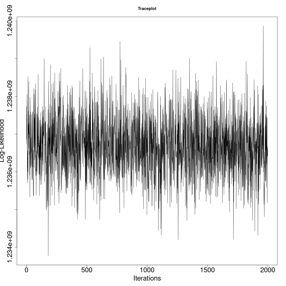
In this section, we provide convergence diagnostics of the MCMC sampler discussed in Section 3.2. Note that most of the variables that are sampled are latent objects and not identifiable. Hence we compute the -likelihood of across the MCMC samples. On these -likelihoods, we show traceplots and Geweke convergence diagnostics (Geweke 1992) as implemented in the coda R package (Plummer et al. 2006). The results are shown in Figure S.10 and they indicate evidence towards good mixing.

References
- Corradin et al. (2021) Corradin, R., Canale, A., and Nipoti, B. (2021). BNPmix: an R package for Bayesian nonparametric modelling via Pitman-Yor mixtures. Journal of Statistical Software, in press.
- Geweke (1992) Geweke, J. (1992). Evaluating the accuracy of sampling-based approaches to the calculations of posterior moments. Bayesian Statistics, 4, 641–649.
- McInnes et al. (2018) McInnes, L., Healy, J., Saul, N., and Großberger, L. (2018). UMAP: Uniform manifold approximation and projection for dimension reduction. Journal of Open Source Software, 3, 861.
- Plummer et al. (2006) Plummer, M., Best, N., Cowles, K., and Vines, K. (2006). CODA: Convergence diagnosis and output analysis for MCMC. R News, 6, 7–11.
- Rand (1971) Rand, W. M. (1971). Objective criteria for the evaluation of clustering methods. Journal of the American Statistical Association, 66, 846–850.