Meta-Model-Based Meta-Policy Optimization

Reinforcement learning (RL) in multi-task problems requires a large number of training samples, and this is a serious obstacle to its practical application (Rakelly et al. 2019). In the real world, we often want a policy that can solve multiple tasks. For example, in robotic arm manipulation (Yu et al. 2019), we may want the policies for controlling the arm to “grasp the wood box,” “grasp the metal box,” “open the door,” and so on. In such multi-task problems, standard RL methods independently learn a policy for individual tasks with millions of training samples (Andrychowicz et al. 2020). This independent policy learning with a large number of samples is often too costly in practical RL applications.

Meta-RL methods have recently gained attention as promising methods to reduce the number of samples required in multi-task problems (Finn et al. 2017). In meta-RL methods, the structure shared in the tasks is learned by using samples collected across the tasks. Once learned, it is leveraged for adapting quickly to new tasks with a small number of samples. Various meta-RL methods have previously been proposed in both model-free and model-based settings.

Many model-free meta-RL methods have been proposed, but they usually require a large number of samples to learn a useful shared structure. In model-free meta-RL methods, the shared structure is learned as being embedded into the parameters of a context-aware policy (Duan et al. 2017; Mishra et al. 2018; Rakelly et al. 2019; Wang et al. 2016), or into the prior of policy parameters (Al-Shedivat et al. 2018; Finn and Levine 2018; Finn et al. 2017; Gupta et al. 2018; Rothfuss et al. 2019; Stadie et al. 2018). The policy adapts to a new task by updating context information or parameters with recent trajectories. Model-free meta-RL methods have better sample efficiency than independently learning a policy for each task. However, these methods still require millions of training samples in total to learn the shared structure sufficiently usefully for the adaptation (Mendonca et al. 2019).

On the other hand, model-based meta-RL methods have been demonstrated to be more sample efficient than model-free counterparts. In model-based meta-RL methods, the shared structure is learned as being embedded into the parameters of a context-aware transition model (Sæmundsson et al. 2018; Perez et al. 2020), or into the prior of the model parameter (Nagabandi et al. 2019a; Nagabandi et al. 2019b). The model adapts to a new task by updating context information or its parameters with recent trajectories. The adapted models are used for action optimization in model predictive control (MPC). In the aforementioned literature, model-based meta-RL methods have been empirically shown to be more sample efficient than model-free meta-RL methods.

Despite these empirical findings, these model-based meta-RL methods lack performance guarantees. Here, the performance guarantee means the theoretical property that specifies the relationship between the planning performance in the model and the actual planning performance in a real environment. Note that the planning performance in the model is generally different from the actual performance due to the model bias. That is, even if planning performs well in the model, it does not necessarily perform well in a real environment. Such a performance guarantee for model-based meta-RL methods has not been analyzed in the literature.

In this paper, we propose a model-based meta-RL method called Meta-Model-based Meta-Policy Optimization (M3PO) which is equipped with a performance guarantee (Figure 1). Specifically, we develop M3PO by firstly formulating a meta-RL setting on the basis of partially observable Markov decision processes (POMDPs) in Section 4. Then, in Section 5, we conduct a theoretical analysis to justify the use of branched rollouts, which is a promising model-based rollout method proposed by Janner et al. 2019, in the meta-RL setting. We compare the theorems for performance guarantees of the branched rollouts and full-model based rollouts, which is a naive baseline model-based rollout method, in the meta-RL setting. Our comparison result shows that the performance of the branched rollout is more tightly guaranteed than that of the full model-based rollouts. Based on this, in Section 6 we derive M3PO, a practical method that uses the branch rollouts. Lastly, in Section 7 we experimentally demonstrate the performance of M3PO in continuous-control benchmarks.

We make four primary contributions in both theoretical and practical frontiers.
Theoretical contributions: (1) We provide the performance guarantee for model-based meta-RL (Section 5). To the best of our knowledge, our work is the first attempt to provide a performance guarantee for model-based meta-RL. (2) We conduct theoretical analysis and provide the insight that short-steps branched rollouts are better than full-model based rollouts (Section 5 and Appendix A). We refine analyses in Janner et al. 2019 by considering multiple-model-based rollout factors (Appendix A.1), and extend our analyses results into a meta-RL setting (Section 5). Therefore, our work complements and strengthens their analyses and insight.
Practical contributions: (3) We propose a practical model-based RL method (M3PO) for meta-RL (Section 6) and demonstrate that it outperforms existing meta-RL methods (Section 7). Notably, we demonstrate that M3PO can work successfully even on complex tasks (e.g., Humanoid-direc). (4) We provide a practically interesting finding that, in M3PO (Dyna-style RL method), dynamically adjusting the mixture ratio of real/fictitious training data substantially improves long-term learning performance (Section 7.1 and Appendix A.8). In existing Dyna-style RL methods (e.g. Janner et al. 2019; Shen et al. 2020; Yu et al. 2020), this mixture ratio is fixed during the training phase. Our finding promotes assessing the effect of dynamically adjusting the mixture ratio for the other Dyna-style RL methods to improve these methods.

Meta-RL is a popular approach for solving multi-tasks RL problems. Recently, researchers have formulated meta-RL as solving special cases of POMDPs (Duan et al. 2017; Humplik et al. 2019; Zintgraf et al. 2020). However, the performance guarantee of meta-RL under the POMDPs framework has not been established. In this paper, we presents bounds of the performance of meta-RL under the POMDPs framework.

We derive the above-mentioned performance bound in the context of model-based meta-RL. Existing works have focused on the performance bound of model-based RL (Feinberg et al. 2018; Henaff 2019; Janner et al. 2019; Luo et al. 2018; Rajeswaran et al. 2020), while ignoring model-based meta-RL. Specifically, in existing works, Markov decision processes (MDPs) are assumed, and a meta-RL setting is not discussed.

In this section, we formulate model-based meta-RL as a special case of POMDPs. In our formulation, the hidden state is assumed to be composed by the task and observation: $\mathcal{S}=\mathcal{T}\times\mathcal{O}$. With this assumption, the transition probability, observation probability, and reward function can be written as follows: $p(s_{t+1}|s_{t},a_{t})=p(\tau_{t+1},o_{t+1}|\tau_{t},o_{t},a_{t})$, $p(o_{t+1}|s_{t+1},a_{t})=p(o_{t+1}|\tau_{t+1},o_{t+1},a_{t})=1$ and $r(s_{t},a_{t})=r(\tau_{t},o_{t},a_{t})$. As in Nagabandi et al. 2019a; Nagabandi et al. 2019b, we assume that the task can change during an episode (i.e., the value of $\tau_{t+1}$ is not necessarily equal to that of $\tau_{t}$). In addition, following previous studies (Finn and Levine 2018; Finn et al. 2017; Rakelly et al. 2019), we assume that the task set $\mathcal{T}$ and the initial task distribution $p(\tau_{0})$ do not change in meta-training and meta-testing. Owing to this assumption, in our analysis and method, meta-training and meta-testing can be seen as identical.

We define a parameterized policy and model as $\pi_{\phi}(a_{t}|h_{L:t})$ and $p_{\theta}(r_{t},o_{t+1}|a_{t},h_{L:t})$, respectively. Here, $\phi$ and $\theta$ are learnable parameters, and $h_{L:t}$ is the truncated history $h_{L:t}=\left\{o_{\max(t-L,0)},a_{\max(t-L,0)},...,o_{t}\right\}$, where $L$ is a hyper-parameter. As with Nagabandi et al. 2019a, we use the history for this period for policy and model adaptation. In addition, we assume that $r_{t}$ and $o_{t+1}$ are conditionally independent given $a_{t}$ and $h_{L:t}$, i.e., $p_{\theta}(r_{t},o_{t+1}|a_{t},h_{L:t})=p_{\theta}(r_{t}|a_{t},h_{L:t})\cdot p_{\theta}(o_{t+1}|a_{t},h_{L:t})$. For analysis in the next section, we use the model for the history $p_{\theta}(h_{t+1}|a_{t},h_{t})$ that can be evaluated by using $p_{\theta}(o_{t+1}|a_{t},h_{L:t})$.

We use the parameterized model and policy as shown in Algorithm 1. This algorithm is composed of 1) training the model, 2) collecting trajectories from the real environment, and 3) training policy to maximize the model return $\mathbb{E}_{(a,h)\sim m(\pi_{\phi},p_{\theta},\mathcal{D}_{\text{env}})}\left[R\right]$. Here, $m(\pi_{\phi},p_{\theta},\mathcal{D}_{\text{env}})$ is the history-action visitation probability based upon an abstract model-based rollout scheme, which can be calculated on the basis of $\pi_{\phi}$, $p_{\theta}$, and $\mathcal{D}_{\text{env}}$. In the next section, we will analyze the algorithm equipped with two specific model-based rollout schemes: the full-model-based rollout and branched rollout.

Our model-based meta-RL formulation via POMDPs introduced in this section is summarized in Figure 2. In the following sections, we present theoretical analysis and empirical experiments on the basis of this formulation.

In the previous section, we formulate our meta-RL setting. In this section, we justify the use of the branched rollout in the meta-RL setting. To do so, we show the performance guarantee of the branched rollout can be tighter than that of full-model based rollout in the meta-RL setting.

The performance guarantees is defined as “planning performance in a real environment $\geq$ planning performance in the model – discrepancy.” Formally, it is represented as:

Here, $\mathbb{E}_{a\sim\pi_{\phi},h\sim p}\left[R\right]$ is a true return (i.e., the planning performance in the real environment). $\mathbb{E}_{(a,h)\sim m(\pi_{\phi},p_{\theta},\mathcal{D}_{\text{env}})}\left[R\right]$ is a model return (i.e., the planning performance in the model). $C(\epsilon_{m},\epsilon_{\pi})$ is the discrepancy between the returns, which can be expressed as the function of two error quantities $\epsilon_{m}$ and $\epsilon_{\pi}$.

In the following, we firstly provide the performance guarantees in the meta-RL setting by deriving the discrepancies $C(\epsilon_{m},\epsilon_{\pi})$ of the full model-based and branched rollouts. Then, we analyze these discrepancies and show that the discrepancy of the branched rollout can yield a tighter performance guarantee than that of the full model-based rollout.

In the previous section, we demonstrated the usefulness of the branched rollout. In this section, we propose Meta-Model-Based Meta-Policy Optimization¹¹ 1 The “meta-model” and “meta-policy” come from the use of $p_{\theta}(r_{t},o_{t+1}|a_{t},h_{L:t})$ and $\pi_{\phi}(a_{t}|h_{L:t})$ in this method. Following previous work (Clavera et al. 2018), we refer to this type of history-conditioned policy as a meta-policy. Similarly, we refer to this type of history-conditioned model as a meta-model. (M3PO), which is a model-based meta-RL method with the branched rollout.

M3PO is described in Algorithm 2. In line 3, the model is learned via maximum likelihood estimation. In line 5, trajectories are collected from the environment with policy $\pi_{\phi}$ and stored into the environment dataset $\mathcal{D}_{\text{env}}$. In lines 6–9, $k$-step branched rollouts are run to generate fictitious trajectories, and the generated ones are stored into the model dataset $\mathcal{D}_{\text{model}}$. In lines 10–12, the policy $\pi_{\phi}$ is learned to improve the model return.

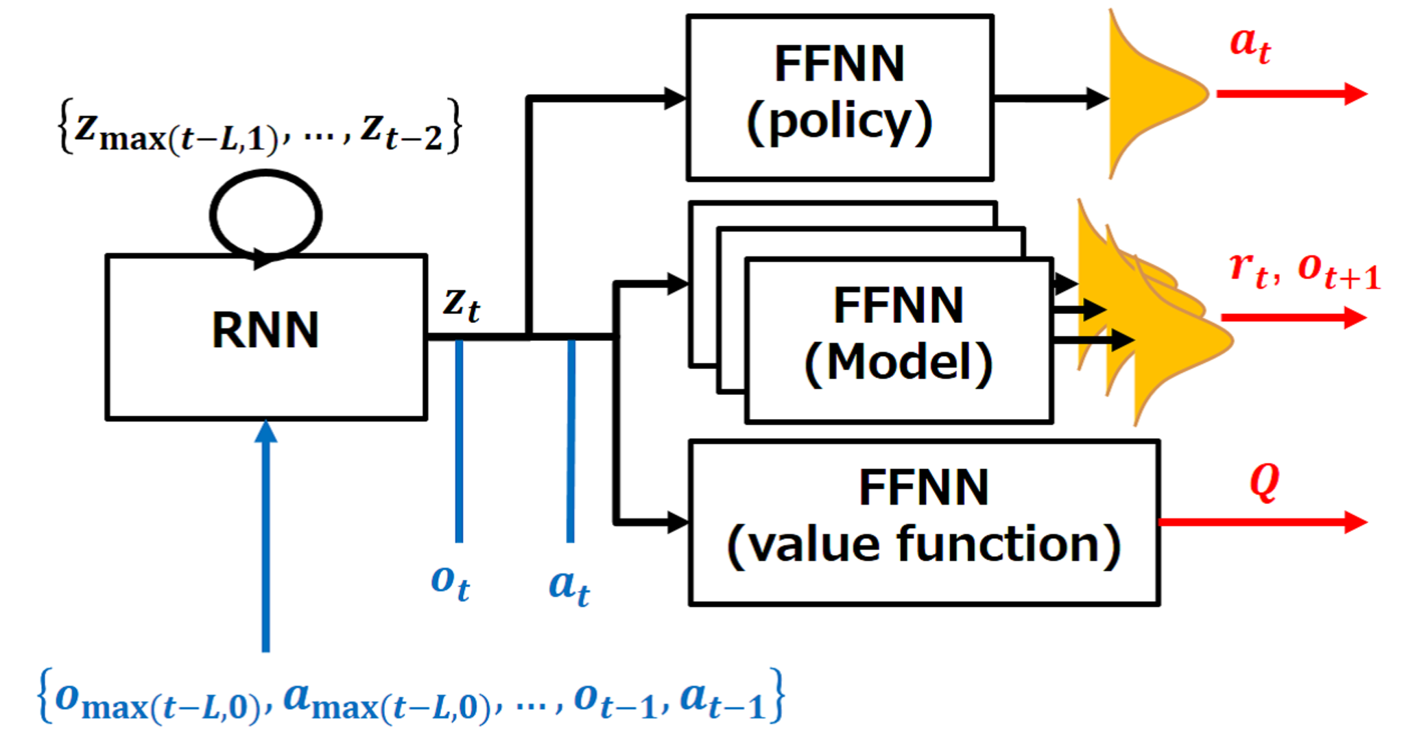
The model is implemented as a bootstrap ensemble of $B$ diagonal Gaussian distributions: $p_{\theta}(r_{t},o_{t+1}|a_{t},h_{L:t})=\frac{1}{B}\sum_{i=1}^{B}\mathcal{N}\left(r_{t+1},o_{t+1}|\mu_{\theta}^{i}\left(a_{t},h_{L:t}\right),\sigma_{\theta}^{i}\left(a_{t},h_{L:t}\right)\right)$. Here, $\mu_{\theta}^{i}$ and $\sigma_{\theta}^{i}$ are the mean and standard deviation, respectively. The model ensemble technique is used to consider both epistemic and aleatoric uncertainty of the model into prediction (Chua et al. 2018). $\mu_{\theta}^{i}$ and $\sigma_{\theta}^{i}$ are implemented with a recurrent neural network (RNN) and a feed-forward neural network (FFNN). At each prediction, $\{o_{\max(t-L,0)},a_{\max(t-L,0)},...,o_{t-1},a_{t-1}\}$ in $h_{L:t}$ is fed to the RNN. Then its hidden-unit outputs $z_{t}$ are fed to the FFNN together with $o_{t}$ and $a_{t}$. The FFNN outputs the mean and standard deviation of the Gaussian distribution, and the next observation and reward are sampled from its ensemble.

The policy is implemented as $\pi_{\phi}(a_{t}|h_{L:t})=\mathcal{N}\left(a_{t}|\mu_{\phi}\left(h_{L:t}\right),\sigma_{\phi}\left(h_{L:t}\right)\right)$. Here, $\mu_{\phi}$ and $\sigma_{\phi}$ are the mean and standard deviation, respectively. The network architecture for them is the same as that for the model, except that the former does not contain $a_{t}$ as input. To train $\phi$, we use a soft-value policy improvement objective (Haarnoja et al. 2018): $J_{\mathcal{D}_{\text{model}}}(\phi)=\mathbb{E}_{h_{L:t}\sim\mathcal{D}_{\text{model}}}\left[D_{KL}\left(\pi_{\phi}||\exp\left(Q-V\right)\right)\right]$. Here, $D_{KL}$ is the Kullback-Leibler divergence, and $Q$ and $V$ are soft-value functions: $Q(a_{t},h_{L:t})=\mathbb{E}_{(r_{t},h_{L:t+1})\sim\mathcal{D}_{\text{model}}}\left[r_{t}+\gamma V(h_{L:t+1})|a_{t},h_{L:t}\right]$ and $V(h_{L:t})=\mathbb{E}_{a\sim\pi_{\phi}}\left[Q(a,h_{L:t})-\log\pi_{\phi}(a|h_{L:t})|h_{L:t}\right]$. The network architecture for $Q$ is identical to that for the model. We do not prepare the network for $V$, and it is directly calculated by using $Q$ and $\pi_{\phi}$.

Figure 5 gives a summary of our implementation of the model, policy and value network for M3PO.

In this section, we report our experiments ²² 2 Source code to replicate the experiments is available at https://github.com/TakuyaHiraoka/Meta-Model-Based-Meta-Policy-Optimization.

In this paper, we analyzed the performance guarantee of the model-based meta-reinforcement learning (RL) method. We first formulated model-based meta-RL as solving a special case of partially observable Markov decision processes. We then theoretically analyzed the performance guarantee of the branched rollout in the meta-RL setting. We showed that the branched rollout has a more tightly guaranteed performance than the full model-based rollouts. Motivated by the theoretical result, we proposed Meta-Model-Based Meta-Policy Optimization (M3PO), a practical model-based meta-RL method based on branched rollouts. Our experimental results show that M3PO outperforms PEARL and L2A.

References

• Al-Shedivat et al. (2018) Maruan Al-Shedivat, Trapit Bansal, Yuri Burda, Ilya Sutskever, Igor Mordatch, and Pieter Abbeel. Continuous adaptation via meta-learning in nonstationary and competitive environments. In Proc. ICLR, 2018.
• Andrychowicz et al. (2020) Marcin Andrychowicz, Bowen Baker, Maciek Chociej, Rafal Józefowicz, Bob McGrew, Jakub Pachocki, Arthur Petron, Matthias Plappert, Glenn Powell, Alex Ray, Jonas Schneider, Szymon Sidor, Josh Tobin, Peter Welinder, Lilian Weng, and Wojciech Zaremba. Learning dexterous in-hand manipulation. The International Journal of Robotics Research, 39(1):3–20, 2020. 10.1177/0278364919887447.
• Cho et al. (2014) Kyunghyun Cho, Bart Van Merriënboer, Caglar Gulcehre, Dzmitry Bahdanau, Fethi Bougares, Holger Schwenk, and Yoshua Bengio. Learning phrase representations using RNN encoder-decoder for statistical machine translation. In Proc. EMNLP, 2014.
• Chua et al. (2018) Kurtland Chua, Roberto Calandra, Rowan McAllister, and Sergey Levine. Deep reinforcement learning in a handful of trials using probabilistic dynamics models. In Proc. NeurIPS, 2018.
• Clavera et al. (2018) Ignasi Clavera, Jonas Rothfuss, John Schulman, Yasuhiro Fujita, Tamim Asfour, and Pieter Abbeel. Model-based reinforcement learning via meta-policy optimization. In Proc. CoRL, pages 617–629, 2018.
• Duan et al. (2017) Yan Duan, John Schulman, Xi Chen, Peter L Bartlett, Ilya Sutskever, and Pieter Abbeel. RL2: Fast reinforcement learning via slow reinforcement learning. In Proc. ICLR, 2017.
• Feinberg et al. (2018) Vladimir Feinberg, Alvin Wan, Ion Stoica, Michael I. Jordan, Joseph E. Gonzalez, and Sergey Levine. Model-based value expansion for efficient model-free reinforcement learning. In Proc. ICML, 2018.
• Finn and Levine (2018) Chelsea Finn and Sergey Levine. Meta-learning and universality: Deep representations and gradient descent can approximate any learning algorithm. In Proc. ICLR, 2018.
• Finn et al. (2017) Chelsea Finn, Pieter Abbeel, and Sergey Levine. Model-agnostic meta-learning for fast adaptation of deep networks. In Proc. ICML, pages 1126–1135, 2017.
• Gupta et al. (2018) Abhishek Gupta, Russell Mendonca, YuXuan Liu, Pieter Abbeel, and Sergey Levine. Meta-reinforcement learning of structured exploration strategies. In Proc. NeurIPS, 2018.
• Haarnoja et al. (2018) Tuomas Haarnoja, Aurick Zhou, Pieter Abbeel, and Sergey Levine. Soft actor-critic: Off-policy maximum entropy deep reinforcement learning with a stochastic actor. In Proc. ICML, pages 1856–1865, 2018.
• Henaff (2019) Mikael Henaff. Explicit explore-exploit algorithms in continuous state spaces. In Proc. NeurIPS, 2019.
• Humplik et al. (2019) Jan Humplik, Alexandre Galashov, Leonard Hasenclever, Pedro A Ortega, Yee Whye Teh, and Nicolas Heess. Meta reinforcement learning as task inference. arXiv preprint arXiv:1905.06424, 2019.
• Janner et al. (2019) Michael Janner, Justin Fu, Marvin Zhang, and Sergey Levine. When to trust your model: Model-based policy optimization. In Proc. NeurIPS, 2019.
• Luo et al. (2018) Yuping Luo, Huazhe Xu, Yuanzhi Li, Yuandong Tian, Trevor Darrell, and Tengyu Ma. Algorithmic framework for model-based deep reinforcement learning with theoretical guarantees. In Proc. ICLR, 2018.
• Mendonca et al. (2019) Russell Mendonca, Abhishek Gupta, Rosen Kralev, Pieter Abbeel, Sergey Levine, and Chelsea Finn. Guided meta-policy search. In Proc. NeurIPS, pages 9653–9664, 2019.
• Mishra et al. (2018) Nikhil Mishra, Mostafa Rohaninejad, Xi Chen, and Pieter Abbeel. A simple neural attentive meta-learner. In Proc. ICLR, 2018.
• Nagabandi et al. (2019a) Anusha Nagabandi, Ignasi Clavera, Simin Liu, Ronald S Fearing, Pieter Abbeel, Sergey Levine, and Chelsea Finn. Learning to adapt in dynamic, real-world environments via meta-reinforcement learning. In Proc. ICLR, 2019a.
• Nagabandi et al. (2019b) Anusha Nagabandi, Chelsea Finn, and Sergey Levine. Deep online learning via meta-learning: Continual adaptation for model-based RL. In Proc. ICLR, 2019b.
• Perez et al. (2020) Christian F Perez, Felipe Petroski Such, and Theofanis Karaletsos. Generalized hidden parameter MDPs transferable model-based RL in a handful of trials. In Proc. AAAI, 2020.
• Rajeswaran et al. (2020) Aravind Rajeswaran, Igor Mordatch, and Vikash Kumar. A game theoretic framework for model based reinforcement learning, 2020.
• Rakelly et al. (2019) Kate Rakelly, Aurick Zhou, Chelsea Finn, Sergey Levine, and Deirdre Quillen. Efficient off-policy meta-reinforcement learning via probabilistic context variables. In Proc. ICML, pages 5331–5340, 2019.
• Ramachandran et al. (2017) Prajit Ramachandran, Barret Zoph, and Quoc V Le. Searching for activation functions. arXiv preprint arXiv:1710.05941, 2017.
• Rothfuss et al. (2019) Jonas Rothfuss, Dennis Lee, Ignasi Clavera, Tamim Asfour, and Pieter Abbeel. ProMP: Proximal meta-policy search. In Proc. ICLR, 2019.
• Sæmundsson et al. (2018) Steindór Sæmundsson, Katja Hofmann, and Marc Peter Deisenroth. Meta reinforcement learning with latent variable Gaussian processes. arXiv preprint arXiv:1803.07551, 2018.
• Shen et al. (2020) Jian Shen, Han Zhao, Weinan Zhang, and Yong Yu. Model-based policy optimization with unsupervised model adaptation. In Proc. NeurIPS, 2020.
• Silver and Veness (2010) David Silver and Joel Veness. Monte-Carlo planning in large POMDPs. In Proc. NIPS, pages 2164–2172, 2010.
• Stadie et al. (2018) Bradly C Stadie, Ge Yang, Rein Houthooft, Xi Chen, Yan Duan, Yuhuai Wu, Pieter Abbeel, and Ilya Sutskever. Some considerations on learning to explore via meta-reinforcement learning. arXiv preprint arXiv:1803.01118, 2018.
• Sutton (1991) Richard S Sutton. Dyna, an integrated architecture for learning, planning, and reacting. ACM Sigart Bulletin, 2(4):160–163, 1991.
• Todorov et al. (2012) Emanuel Todorov, Tom Erez, and Yuval Tassa. MuJoCo: A physics engine for model-based control. In Proc. IROS, pages 5026–5033. IEEE, 2012.
• Wang et al. (2016) Jane X Wang, Zeb Kurth-Nelson, Dhruva Tirumala, Hubert Soyer, Joel Z Leibo, Remi Munos, Charles Blundell, Dharshan Kumaran, and Matt Botvinick. Learning to reinforcement learn. arXiv preprint arXiv:1611.05763, 2016.
• Williams et al. (2015) Grady Williams, Andrew Aldrich, and Evangelos Theodorou. Model predictive path integral control using covariance variable importance sampling. arXiv preprint arXiv:1509.01149, 2015.
• Yu et al. (2019) Tianhe Yu, Deirdre Quillen, Zhanpeng He, Ryan Julian, Karol Hausman, Chelsea Finn, and Sergey Levine. Meta-world: A benchmark and evaluation for multi-task and meta reinforcement learning. In Proc. CoRL, 2019.
• Yu et al. (2020) Tianhe Yu, Garrett Thomas, Lantao Yu, Stefano Ermon, James Y Zou, Sergey Levine, Chelsea Finn, and Tengyu Ma. MOPO: model-based offline policy optimization. In Proc. NeurIPS, 2020.
• Zintgraf et al. (2020) Luisa Zintgraf, Kyriacos Shiarlis, Maximilian Igl, Sebastian Schulze, Yarin Gal, Katja Hofmann, and Shimon Whiteson. VariBAD: A very good method for Bayes-adaptive deep RL via meta-learning. In Proc. ICLR, 2020.
Appendix A
A.1 The relation of returns (performance guarantee) under kk-step branched rollouts in Markov decision processes
In this section, we analyze the relation of a true return and a model return in an MDP, which is defined by a tuple ⟨𝒮,𝒜,r,γ,pst⟩\langle\mathcal{S},\mathcal{A},r,\gamma,p_{\text{st}}\rangle. Here, 𝒮\mathcal{S} is a set of states, 𝒜\mathcal{A} is a set of actions, pst=𝒮×𝒮×𝒜→[0,1]p_{\text{st}}=\mathcal{S}\times\mathcal{S}\times\mathcal{A}\rightarrow[0,1] is the state transition probability, r:𝒮×𝒜→ℝr:\mathcal{S}\times\mathcal{A}\rightarrow\mathbb{R} is a reward function and γ∈[0,1)\gamma\in[0,1) is a discount factor. At time step tt, the state transition probability and reward function are used as p⁡(st|st−1,at−1)p(s_{t}|s_{t-1},a_{t-1}) and r⁡(st,at)r(s_{t},~a_{t}), respectively. The true return is defined as 𝔼a∼π,s∼p[R=∑t=0∞γtrt]\mathbb{E}_{a\sim\pi,s\sim p}\left[R=\sum_{t=0}^{\infty}\gamma^{t}r_{t}\right], where π\pi is the agent’s current policy. In addition, the model return is defined by 𝔼(a,s)∼mb​(π,pθ,𝒟env)​[R]\mathbb{E}_{(a,s)\sim m_{b}(\pi,p_{\theta},\mathcal{D}_{\text{env}})}\left[R\right], where m⁡(π,pθ,𝒟env)m(\pi,p_{\theta},\mathcal{D}_{\text{env}}) is the state-action visitation probability based upon an abstract model-based rollout method, which can be calculated on the basis of the π\pi, pθp_{\theta}, and 𝒟env\mathcal{D}_{\text{env}}. pθp_{\theta} is the predictive model for the next state. 𝒟env\mathcal{D}_{\text{env}} is the dataset in which the real trajectories collected by a data collection policy π𝒟\pi_{\mathcal{D}} is stored.
We analyze the relation of the returns, which takes the form of
𝔼a∼π,s∼p​[R]≥𝔼(a,s)∼m⁡(π,pθ,𝒟env)​[R]−C⁡(ϵm,ϵπ),\displaystyle\mathbb{E}_{a\sim\pi,s\sim p}\left[R\right]\geq\mathbb{E}_{(a,s)\sim m(\pi,p_{\theta},\mathcal{D}_{\text{env}})}\left[R\right]-C(\epsilon_{m},\epsilon_{\pi}),
where C⁡(ϵm,ϵπ)C(\epsilon_{m},\epsilon_{\pi}) is the discrepancy between the returns, which can be expressed as the function of two error quantities ϵm\epsilon_{m} and ϵπ\epsilon_{\pi}. Here, ϵm=maxt𝔼at∼π𝒟,st∼p[DTV(p(st+1|st,at)||pθ(st+1|st,at))]\epsilon_{m}=\max_{t}\mathbb{E}_{a_{t}\sim\pi_{\mathcal{D}},s_{t}\sim p}\left[D_{\text{TV}}\left(p(s_{t+1}|s_{t},a_{t})||p_{\theta}(s_{t+1}|s_{t},a_{t})\right)\right] and ϵπ=maxstDTV(π(at|st)||π𝒟(at|st))\epsilon_{\pi}=\max_{s_{t}}D_{\text{TV}}\left(\pi(a_{t}|s_{t})||\pi_{\mathcal{D}}(a_{t}|s_{t})\right). In addition, we define the upper bounds of the reward scale as rmax>maxs,a⁡|r⁡(s,a)|r_{\text{max}}>\max_{s,a}|r(s,a)|. Note that, in this section, to discuss the MDP case, we are overriding the definition of the variables and functions that were defined for the POMDP case in the main content.
Janner et al. 2019 analyzed the relations of the returns under the full-model-based rollout and that under the branched rollout in the MDP:
Theorem 4.1. in Janner et al. 2019. Under the full-model-based rollout in the MDP, the following inequality holds,
𝔼a∼π,s∼p​[R]≥𝔼(a,s)∼mf​(π,pθ,𝒟env)​[R]−2​rmax​{γ(1−γ)2​(ϵm+2​ϵπ)+2(1−γ)​ϵm},\mathbb{E}_{a\sim\pi,s\sim p}\left[R\right]\geq\mathbb{E}_{(a,s)\sim m_{f}(\pi,p_{\theta},\mathcal{D}_{\text{env}})}\left[R\right]-2r_{\text{max}}\left\{\frac{\gamma}{(1-\gamma)^{2}}(\epsilon_{m}+2\epsilon_{\pi})+\frac{2}{(1-\gamma)}\epsilon_{m}\right\}, (2)
where 𝔼(a,s)∼mf​(π,pθ,𝒟env)​[R]\mathbb{E}_{(a,s)\sim m_{f}(\pi,p_{\theta},\mathcal{D}_{\text{env}})}\left[R\right] is the model return under the full-model-based rollout. mf​(πϕ,pθ,𝒟env)m_{f}(\pi_{\phi},p_{\theta},\mathcal{D}_{\text{env}}) is the state-action visitation probability under the full model-based rollout method.
Theorem 4.2. in Janner et al. 2019. Under the branched rollout in the MDP, the following inequality holds,
𝔼a∼π,s∼p​[R]≥𝔼(a,s)∼mb​(π,pθ,𝒟env)​[R]−2​rmax​{γk+1(1−γ)2​ϵπ+γk+2(1−γ)​ϵπ+k1−γ​(ϵm+2​ϵπ)},\mathbb{E}_{a\sim\pi,s\sim p}\left[R\right]\geq\mathbb{E}_{(a,s)\sim m_{b}(\pi,p_{\theta},\mathcal{D}_{\text{env}})}\left[R\right]-2r_{\text{max}}\left\{\frac{\gamma^{k+1}}{(1-\gamma)^{2}}\epsilon_{\pi}+\frac{\gamma^{k}+2}{(1-\gamma)}\epsilon_{\pi}+\frac{k}{1-\gamma}(\epsilon_{m}+2\epsilon_{\pi})\right\}, (3)
where 𝔼(a,s)∼mb​(π,pθ,𝒟env)​[R]\mathbb{E}_{(a,s)\sim m_{b}(\pi,p_{\theta},\mathcal{D}_{\text{env}})}\left[R\right] is the model return under the branched rollout. mb​(πϕ,pθ,𝒟env)m_{b}(\pi_{\phi},p_{\theta},\mathcal{D}_{\text{env}}) is the state-action visitation probability under the branched rollout method.
The notion of mb​(π,pθ,𝒟env)m_{b}(\pi,p_{\theta},\mathcal{D}_{\text{env}}) in the analyses in Janner et al. 2019 and our case are summarized in Figure 10. In the branched rollout method, the real trajectories are uniformly sampled from 𝒟env\mathcal{D}_{\text{env}}, and then starting from the sampled trajectories, kk-step model-based rollouts under π\pi and pθp_{\theta} are run. Then, the fictitious trajectories generated by the branched rollout are stored in a model dataset DmodelD_{\text{model}} 33 3 Here, when the trajectories are stored in DmodelD_{\text{model}}, the states in the trajectories are augmented with time step information to deal with the state transition depending on the time step.. The distribution of the trajectories stored in DmodelD_{\text{model}} is used as mb​(π,pθ,𝒟env)m_{b}(\pi,p_{\theta},\mathcal{D}_{\text{env}}). In Figure 10, pπ𝒟​(st,at)p_{\pi_{\mathcal{D}}}(s_{t},a_{t}) is the state-action visitation probability under pstp_{\text{st}} and πD\pi_{D}. This can be used for the initial state distribution for kk-steps model-based rollouts since the real trajectories are uniformly sampled from 𝒟env\mathcal{D}_{\text{env}}. In addition, pt<k,ibr​(st,at)p_{t<k,i}^{\text{br}}(s_{t},a_{t}) and pt≥k,ibr​(st,at)p_{t\geq k,i}^{\text{br}}(s_{t},a_{t}) are the state-action visitation probabilities that the ii-th yellow fictitious trajectories (nodes) from the bottom at tt follow.
Refer to caption
Figure 10: The notion of mb​(πϕ,pθ,𝒟env)m_{b}(\pi_{\phi},p_{\theta},\mathcal{D}_{\text{env}}). The figure shows the case of the branched rollout method with k=3k=3. The blue nodes represent real trajectories contained in 𝒟env\mathcal{D}_{\text{env}}, and the yellow nodes represent fictitious trajectories generated by kk-step model-based rollouts with π\pi and pθp_{\theta}. The fictitious trajectories are stored in DmodelD_{\text{model}}. The distribution of the trajectories stored in DmodelD_{\text{model}} is used as mb​(π,pθ,𝒟env)m_{b}(\pi,p_{\theta},\mathcal{D}_{\text{env}}). In the analysis (derivation of Theorem 4.2) in Janner et al. 2019, fictitious trajectories of dashed yellow nodes are not stored in 𝒟model\mathcal{D}_{\text{model}}, and thus the state-action visitation probability at each time step is calculated based solely on a single model-based rollout factor. To contrast, in our analysis, these fictitious trajectories are stored in 𝒟model\mathcal{D}_{\text{model}}, and thus the state-action visitation probability at each time step is calculated on the basis of multiple model-based rollout factors.
In the derivation of Theorem 4.2 (more specifically, the proof of Lemma B.4) in Janner et al. 2019, important premises are not properly taken into consideration. In the derivation, state-action visitation probabilities under the branched rollout are affected only by a single model-based rollout factor (see Figure 10). For example, a state-action visitation probability at tt (s.t. t>kt>k) is affected only by the model-based rollout branched from real trajectories at t−kt-k (i.e., pt≥k,0br​(st,at)p_{t\geq k,0}^{\text{br}}(s_{t},a_{t})). However, state-action visitation probabilities (except for ones at t=0t=0 and t=1t=1) should be affected by multiple past model-based rollouts. For example, a state-action visitation probability at tt (s.t. t>kt>k) should be affected by the model-based rollout branched from real trajectories at t−kt-k and ones from t−k+1t-k+1 to t−1t-1 (i.e., pt≥k,0br​(st,at)​…,pt≥k,k−1br​(st,at)p_{t\geq k,0}^{\text{br}}(s_{t},a_{t})...,p_{t\geq k,k-1}^{\text{br}}(s_{t},a_{t})). In addition, in their analysis, they consider that kk is an element of the set of non-negative integers. However, if k=0k=0, the fictitious trajectories for 𝒟model\mathcal{D}_{\text{model}} are not generated, and the distribution of trajectories in 𝒟model\mathcal{D}_{\text{model}} cannot be built. Therefore, kk’s value should not be 0 (it should be an element of the set of non-zero natural numbers ℕ>0\mathbb{N}_{>0}). These oversights of important premises in their analysis induce a large mismatch between those for their theorem (Theorem 4.2) and those made for the actual implementation of the branched rollout (lines 5–8 in Algorithm 2 in Janner et al. 2019).
Hence, we will newly analyze the relation of the returns under the branched rollout method, considering the aforementioned premises more properly. Concretely, we consider the multiple model-based rollout factors for mb​(π,pθ,𝒟env)m_{b}(\pi,p_{\theta},\mathcal{D}_{\text{env}}) (See Figure 10) 44 4 Considering the discussion in the last paragraph, we also limit the range of kk as k∈ℕ>0k\in\mathbb{N}_{>0} in our analysis.. With this consideration, we define the model-return under the branched rollout 𝔼(a,s)∼mb​(π,pθ,𝒟env)​[R]\mathbb{E}_{(a,s)\sim m_{b}(\pi,p_{\theta},\mathcal{D}_{\text{env}})}[R] as:
𝔼(a,s)∼mb​(π,pθ,𝒟env)​[R]\displaystyle\mathbb{E}_{(a,s)\sim m_{b}(\pi,p_{\theta},\mathcal{D}_{\text{env}})}[R] =\displaystyle= ∑s0,a0pπ𝒟​(s0,a0)​r​(s0,a0)+∑t=1k−1∑st,atγt​pt<kbr​(st,at)​r​(st,at)\displaystyle\sum_{s_{0},a_{0}}p_{\pi_{\mathcal{D}}}(s_{0},a_{0})r(s_{0},a_{0})+\sum_{t=1}^{k-1}\sum_{s_{t},a_{t}}\gamma^{t}p_{t<k}^{\text{br}}(s_{t},a_{t})r(s_{t},a_{t}) (4)
+∑t=k∞∑st,atγtpt≥kbr(st,at)r(st,at)\displaystyle+\sum_{t=k}^{\infty}\sum_{s_{t},a_{t}}\gamma^{t}p_{t\geq k}^{\text{br}}(s_{t},a_{t})r(s_{t},a_{t})
pt<kbr​(st,at)\displaystyle p_{t<k}^{\text{br}}(s_{t},a_{t}) =\displaystyle= 1t​∑i=0t−1pt<k,ibr​(st,at)\displaystyle{\color[rgb]{1,0,0}\frac{1}{t}\sum_{i=0}^{t-1}p_{t<k,i}^{\text{br}}(s_{t},a_{t})} (5)
pt≥kbr​(st,at)\displaystyle p_{t\geq k}^{\text{br}}(s_{t},a_{t}) =\displaystyle= 1k​∑i=0k−1pt≥k,ibr​(st,at)\displaystyle{\color[rgb]{1,0,0}\frac{1}{k}\sum_{i=0}^{k-1}p_{t\geq k,i}^{\text{br}}(s_{t},a_{t})} (6)
pt<k,ibr​(st,at)\displaystyle p_{t<k,i}^{\text{br}}(s_{t},a_{t}) =\displaystyle= ∑si,…,st−1∑ai,…,at−1pπ𝒟​(si)​Πj=it−1​pθ​(sj+1|sj,aj)​π​(aj|sj)\displaystyle\sum_{s_{i},...,s_{t-1}}\sum_{a_{i},...,a_{t-1}}p_{\pi_{\mathcal{D}}}(s_{i})\Pi_{j=i}^{t-1}p_{\theta}(s_{j+1}|s_{j},a_{j})\pi(a_{j}|s_{j}) (7)
pt≥k,ibr​(st,at)\displaystyle p_{t\geq k,i}^{\text{br}}(s_{t},a_{t}) =\displaystyle= ∑st−k+i,…,st−1∑at−k+i,…,at−1\displaystyle\sum_{s_{t-k+i},...,s_{t-1}}\sum_{a_{t-k+i},...,a_{t-1}} (8)
pπ𝒟​(st−k+i)​Πj=t−k+it−1​pθ​(sj+1|sj,aj)​π​(aj|sj)\displaystyle p_{\pi_{\mathcal{D}}}(s_{t-k+i})\Pi_{j=t-k+i}^{t-1}p_{\theta}(s_{j+1}|s_{j},a_{j})\pi(a_{j}|s_{j})
Here, pπ𝒟p_{\pi_{\mathcal{D}}} is the state visitation probability under π𝒟\pi_{\mathcal{D}} and pstp_{\text{st}}. The ones modified from Janner et al. 2019 are highlighted in red. In the remaining paragraphs in this section, we will derive the new theorems for the relation of the returns under this definition of the model return.
Before starting the derivation of our theorem, we introduce a useful lemma.
Lemma 1.
Assume that the rollout process in which the policy and dynamics can be switched to other ones at time step tswt_{\text{sw}}. Letting two probabilities be p1p_{1} and p2p_{2}, for 1≤t′≤tsw1\leq t^{\prime}\leq t_{\text{sw}}, we assume that the dynamics distributions are bounded as
ϵm,pre=maxt′Es∼p1[DTV(p1(st′|st′−1,at′−1)||p2(st′|st′−1,at′−1))]\epsilon_{m,\text{pre}}=\max_{t^{\prime}}E_{s\sim p_{1}}\left[D_{\text{TV}}\left(p_{1}(s_{t^{\prime}}|s_{t^{\prime}-1},a_{t^{\prime}-1})||p_{2}(s_{t^{\prime}}|s_{t^{\prime}-1},a_{t^{\prime}-1})\right)\right]. In addition, for tsw<t′≤tt_{\text{sw}}<t^{\prime}\leq t, we assume that the dynamics distributions are bounded as
ϵm,post=maxt′Es∼p1[DTV(p1(st′|st′−1,at′−1)||p2(st′|st′−1,at′−1))]\epsilon_{m,\text{post}}=\max_{t^{\prime}}E_{s\sim p_{1}}\left[D_{\text{TV}}\left(p_{1}(s_{t^{\prime}}|s_{t^{\prime}-1},a_{t^{\prime}-1})||p_{2}(s_{t^{\prime}}|s_{t^{\prime}-1},a_{t^{\prime}-1})\right)\right]. Likewise, the policy divergence is bounded by ϵπ,pre\epsilon_{\pi,\text{pre}} and ϵπ,post\epsilon_{\pi,\text{post}}. Then, the following inequality holds
∑st,at|p1​(st,at)−p2​(st,at)|≤2​(t−tsw)​(ϵm,post+ϵπ,post)+2​tsw​(ϵm,pre+ϵπ,pre)\sum_{s_{t},a_{t}}\left|p_{1}(s_{t},a_{t})-p_{2}(s_{t},a_{t})\right|\leq 2(t-t_{\text{sw}})(\epsilon_{m,\text{post}}+\epsilon_{\pi,\text{post}})+2t_{\text{sw}}(\epsilon_{m,\text{pre}}+\epsilon_{\pi,\text{pre}}) (9)
Proof.
The proof is done in a similar manner to those of Lemma B.1 and B.2 in Janner et al. 2019.
∑st,at|p1​(st,at)−p2​(st,at)|=∑st,at|p1​(st)​p1​(at|st)−p2​(st)​p2​(at|st)|=∑st,at|p1​(st)​p1​(at|st)−p1​(st)​p2​(at|st)+(p1​(st)−p2​(st))​p2​(at|st)|≤∑st,atp1​(st)​|p1​(at|st)−p2​(at|st)|+∑st|p1​(st)−p2​(st)|≤∑st,atp1​(st)​|p1​(at|st)−p2​(at|st)|+∑st,at−1|p1​(st,at−1)−p2​(st,at−1)|=∑st,atp1​(st)​|p1​(at|st)−p2​(at|st)|+∑st,at−1|p1​(at−1)​p1​(st|at−1)−p1​(at−1)​p2​(st|at−1)+(p1​(at−1)−p2​(at−1))​p2​(st|at−1)|≤∑st,atp1​(st)​|p1​(at|st)−p2​(at|st)|+∑st,at−1p1​(at−1)​|p1​(st|at−1)−p2​(st|at−1)|+∑at−1|p1​(at−1)−p2​(at−1)|≤∑st,atp1​(st)​|p1​(at|st)−p2​(at|st)|+∑st,at−1p1​(at−1)​|p1​(st|at−1)−p2​(st|at−1)|+∑st−1,at−1|p1​(st−1,at−1)−p2​(st−1,st−1)|≤2​ϵm,post+2​ϵπ,post+∑st−1,at−1|p1​(st−1,at−1)−p2​(st−1,st−1)|≤2​(t−tsw)​(ϵm,post+ϵπ,post)+∑stsw,atsw|p1​(stsw,atsw)−p2​(stsw,stsw)|≤2​(t−tsw)​(ϵm,post+ϵπ,post)+2​tsw​(ϵm,pre+ϵπ,pre)\sum_{s_{t},a_{t}}\left|p_{1}(s_{t},a_{t})-p_{2}(s_{t},a_{t})\right|=\sum_{s_{t},a_{t}}\left|p_{1}(s_{t})p_{1}(a_{t}|s_{t})-p_{2}(s_{t})p_{2}(a_{t}|s_{t})\right|=\sum_{s_{t},a_{t}}\left|p_{1}(s_{t})p_{1}(a_{t}|s_{t})-p_{1}(s_{t})p_{2}(a_{t}|s_{t})+(p_{1}(s_{t})-p_{2}(s_{t}))p_{2}(a_{t}|s_{t})\right|\leq\sum_{s_{t},a_{t}}p_{1}(s_{t})\left|p_{1}(a_{t}|s_{t})-p_{2}(a_{t}|s_{t})\right|+\sum_{s_{t}}\left|p_{1}(s_{t})-p_{2}(s_{t})\right|\leq\sum_{s_{t},a_{t}}p_{1}(s_{t})\left|p_{1}(a_{t}|s_{t})-p_{2}(a_{t}|s_{t})\right|+\sum_{s_{t},a_{t-1}}\left|p_{1}(s_{t},a_{t-1})-p_{2}(s_{t},a_{t-1})\right|=\sum_{s_{t},a_{t}}p_{1}(s_{t})\left|p_{1}(a_{t}|s_{t})-p_{2}(a_{t}|s_{t})\right|\\ ~+\sum_{s_{t},a_{t-1}}\left|p_{1}(a_{t-1})p_{1}(s_{t}|a_{t-1})-p_{1}(a_{t-1})p_{2}(s_{t}|a_{t-1})+(p_{1}(a_{t-1})-p_{2}(a_{t-1}))p_{2}(s_{t}|a_{t-1})\right|\\ \leq\sum_{s_{t},a_{t}}p_{1}(s_{t})\left|p_{1}(a_{t}|s_{t})-p_{2}(a_{t}|s_{t})\right|+\sum_{s_{t},a_{t-1}}p_{1}(a_{t-1})\left|p_{1}(s_{t}|a_{t-1})-p_{2}(s_{t}|a_{t-1})\right|\\ ~+\sum_{a_{t-1}}\left|p_{1}(a_{t-1})-p_{2}(a_{t-1})\right|\leq\sum_{s_{t},a_{t}}p_{1}(s_{t})\left|p_{1}(a_{t}|s_{t})-p_{2}(a_{t}|s_{t})\right|+\sum_{s_{t},a_{t-1}}p_{1}(a_{t-1})\left|p_{1}(s_{t}|a_{t-1})-p_{2}(s_{t}|a_{t-1})\right|\\ ~+\sum_{s_{t-1},a_{t-1}}\left|p_{1}(s_{t-1},a_{t-1})-p_{2}(s_{t-1},s_{t-1})\right|\leq 2\epsilon_{m,\text{post}}+2\epsilon_{\pi,\text{post}}+\sum_{s_{t-1},a_{t-1}}\left|p_{1}(s_{t-1},a_{t-1})-p_{2}(s_{t-1},s_{t-1})\right|\leq 2(t-t_{\text{sw}})(\epsilon_{m,\text{post}}+\epsilon_{\pi,\text{post}})+\sum_{s_{t_{\text{sw}}},a_{t_{\text{sw}}}}\left|p_{1}(s_{t_{\text{sw}}},a_{t_{\text{sw}}})-p_{2}(s_{t_{\text{sw}}},s_{t_{\text{sw}}})\right|\leq 2(t-t_{\text{sw}})(\epsilon_{m,\text{post}}+\epsilon_{\pi,\text{post}})+2t_{\text{sw}}(\epsilon_{m,\text{pre}}+\epsilon_{\pi,\text{pre}}) (10)
∎
Now, we start the derivation of our theorems.
Theorem 3.
Under the k∈ℕ>0k\in\mathbb{N}_{>0} steps branched rollouts in the MDP ⟨𝒮,𝒜,r,γ,pst⟩\langle\mathcal{S},\mathcal{A},r,\gamma,p_{\text{st}}\rangle, given the bound of the errors ϵm=maxt𝔼at∼π𝒟,st∼p[DTV(p(st+1|st,at)||pθ(st+1|st,at))]\epsilon_{m}=\max_{t}\mathbb{E}_{a_{t}\sim\pi_{\mathcal{D}},s_{t}\sim p}\left[D_{\text{TV}}\left(p(s_{t+1}|s_{t},a_{t})||p_{\theta}(s_{t+1}|s_{t},a_{t})\right)\right] and ϵπ=maxstDTV(π(at|st)||π𝒟(at|st))\epsilon_{\pi}=\max_{s_{t}}D_{\text{TV}}\left(\pi(a_{t}|s_{t})||\pi_{\mathcal{D}}(a_{t}|s_{t})\right), the following inequality holds,
𝔼a∼π,s∼p​[R]≥𝔼(a,s)∼mb​(π,pθ,𝒟env)​[R]−rmax​{1+γ2(1−γ)2​2​ϵπ+γ−k​γk+(k−1)​γk+1(1−γ)2​(ϵπ+ϵm)+γk−γγ−1​(ϵπ+ϵm)+γk1−γ​(k+1)​(ϵπ+ϵm)}.\mathbb{E}_{a\sim\pi,s\sim p}\left[R\right]\geq\mathbb{E}_{(a,s)\sim m_{b}(\pi,p_{\theta},\mathcal{D}_{\text{env}})}\left[R\right]-r_{\text{max}}\left\{\frac{1+\gamma^{2}}{(1-\gamma)^{2}}2\epsilon_{\pi}+\frac{\gamma-k\gamma^{k}+(k-1)\gamma^{k+1}}{(1-\gamma)^{2}}\left(\epsilon_{\pi}+\epsilon_{m}\right)\\ +\frac{\gamma^{k}-\gamma}{\gamma-1}(\epsilon_{\pi}+\epsilon_{m})+\frac{\gamma^{k}}{1-\gamma}(k+1)(\epsilon_{\pi}+\epsilon_{m})\right\}. (11)