Shallow Neural Hawkes: Non-parametric kernel estimation for Hawkes processes
Abstract
Multi-dimensional Hawkes process (MHP) is a class of self and mutually exciting point processes that find wide range of applications – from prediction of earthquakes to modelling of order books in high frequency trading. This paper makes two major contributions, we first find an unbiased estimator for the log-likelihood estimator of the Hawkes process to enable efficient use of the stochastic gradient descent method for maximum likelihood estimation. The second contribution is, we propose a specific single hidden layered neural network for the non-parametric estimation of the underlying kernels of the MHP. We evaluate the proposed model on both synthetic and real datasets, and find the method has comparable or better performance than existing estimation methods. The use of shallow neural network ensures that we do not compromise on the interpretability of the Hawkes model, while at the same time have the flexibility to estimate any non-standard Hawkes excitation kernel.
1 Introduction
Hawkes processes Hawkes 1971 are temporal point processes in which the intensity depends on the process history with an excitation mechanism. It is well-known for studying seismic events Ogata 1999, financial analysis Filimonov and Sornette 2012, Bacry et al. 2015 and modelling social interactions Crane and Sornette 2008, Blundell et al. 2012, Zhou et al. 2013. In the field of biology, it is used to study genomic events along DNA sequences Reynaud-Bouret et al. 2010. MHP has also been used to model crime Mohler et al. 2011 and study the pattern of civilian deaths in Iraq Lewis et al. 2012. The primary concern in modelling Hawkes process is the estimation of link function or excitation kernel. A common practice has been to assume a parametric form of the excitation kernel, the most common being exponential and power-law decay kernels, and then using maximum likelihood estimation Ozaki 1979 to determine the optimal values of the parameters.
Formally, the multi-dimensional Hawkes process is defined by a -dimensional point process with the conditional intensity for the -th dimension expressed as,
| (1) |
where is the exogenous base intensity for the -th node and is independent of the history. are called the excitation kernels that quantify the magnitude of excitation of the base intensity of the -th node over time due to the past events from node These kernel functions are positive and causal (their support is within ). Inferring a Hawkes process requires estimating the base intensity and its kernels functions either by assuming a parametric form for the kernels or in a non-parametric fashion. Recent developments focus on data-driven, non-parametric estimations of MHP to capture the general shape of the kernel and increase flexibility of the model.
In general, the kernels as well as the base intensity can be estimated by maximizing the associated log-likelihood function. However, as will be discussed further in Section 3, the challenge is that the log-likelihood function contains the integral of intensity function that depends on the values of the kernels over the whole time interval. In this paper we present an unbiased estimator for the log-likelihood function of the MHP, which makes application of SGD for maximum likelihood estimation straightforward. It should be noted that as the log-likelihood function for MHP is usually non-convex in the parameter space, even for the basic exponential kernels, the SGD or other optimization methods do not guarantee a global maximum. However, in our experiments we observe that SGD, with ADAM, Kingma and Ba 2014, used for the adaptive learning rates, with prescribed choice of initialization gets sufficiently close to the optimal parameters in few iterations.
The main contribution of the paper is development of a feed-forward neural network based non-parametric approach to estimate the kernels of MHP. Specifically each excitation kernel of the MHP is modelled as a separate feed-forward network with a single hidden layer. The weights of the different networks are coupled with each other in the likelihood function and the optimal weights are then determined using the batch SGD with objective to maximize the log likelihood. The choice of using a shallow –a single hidden layered– neural network is to ensure that, on one hand a closed form for the time integrated value of the excitation kernels can be obtained, while at the same time –by the virtue of the universal approximation theorem– have the ability to approximate any excitation kernel to arbitrary precision. In this paper we only consider the excitation effect of new arrivals, i.e. the output of the excitation kernel ranges in and a fixed base intensity. We test our model against few state-of-the-art non-parametric estimation methods for MHP. The method is tested against both synthetic as well as real data set. For real dataset we consider the high frequency data of buy and sell market orders from Binance cryptoexchange. We find that the performance of our method, which we call the Shallow Neural Hawkes (SNH) is comparable or better than benchmark models. We see a distinct advantage of our approach, in comparison to the use of recurrent neural networks to model MHP, as we do not lose the interpretability of MHP by recovering the underlying excitation kernels. Another advantage our method is that a closed form expression for the integrated kernel functions is obtained, which –for instance– histogram based non-parametric methods would require discrete time approximations.
2 Related Work
In many real world applications the flexibility of Hawkes process is enhanced by the use of non-parametric models. The first non-parametric model of one dimensional Hawkes processes was proposed in Lewis and Mohler 2011 , based on ordinary differential equation (ODE). The first extension of non-parametric kernels to multi-dimensional case was provided in Zhou et al. 2013. They developed an algorithm to learn the decay kernels by using Euler-Lagrange equations for optimization, in infinite dimensional functional space. Determined to model large amount of data, a non-parametric method based on solving the Wiener-Hopf equation using a Gaussian quadrature method was introduced in Bacry and Muzy 2014. Motivated by the branching property of Hawkes process Zhuang et al. 2002, an Expectation-Maximization(EM) algorithm was developed in Marsan and Lengline 2008 for non-parametric estimation of decay kernel and background intensity.
The methods close to our approach include the MEMIP (Markovian Estimation of Mutually Interacting Processes) Lemonnier and Vayatis 2014 that makes use of polynomial approximation theory and self concordant analysis to learn the kernels and the base intensities. While the non-parametric models in (Lemonnier and Vayatis 2014; Zhou et al. 2013) represent excitation functions as a set of basis functions, a guidance for the selection process of basis functions is provided in Xu et al. 2016. Both Xu et al. 2016 and Salehi et al. 2019 express the excitation kernels as sum of Gaussian basis kernels, the former uses sparse group-lasso regularizer and is suitable for large datasets, while the latter uses variational expectation-maximization and is suitable for a handful of datasets. The approach presented in this paper is similar, as the excitation function is expressed as a non-parametric function, specifically as exponential of sum of rectified linear units (ReLUs).
In a relatively new study of temporal point processes, the authors in Du et al. 2016 develop a recurrent neural network to model point processes and learn influences from event history. The authors in Mei and Eisner 2017 develop a novel continuous-time LSTM to model self-modulating Hawkes processes. This setting can capture the exciting and inhibiting effects of past events on future and allow the background intensity to take negative values corresponding to delayed response or inertia of some events. Compared to the approach of expressing each excitation kernel as a neural network, LSTM might be less desirable when there is a greater focus of the interpretability of the MHP, for instance for learning the Granger causality graph. We also significantly simplify the SGD formulation as compared to Mei and Eisner 2017, where one has to rely on simulations to obtain the gradients, while in Du et al. 2016 numerical integration is needed to obtain the necessary gradients of the log likelihood.
3 Preliminary Definitions
A -dimensional MHP is a collection of univariate counting processes The realization of MHP over an observation period consists of a sequence of discrete events where is the timestamp of the -th event and is the label of corresponding dimension in which the event occurred. The conditional intensity process for the th dimension is given by Equation 1. Often the Hawkes kernels are assumed to be exponential function of the form and the base intensity is assumed to be constant. In this paper we assume that can be an arbitrary continuous function while is a positive constant.
We denote the parameters of the multi-dimensional Hawkes process in a matrix form as for the base intensity, and for the excitation kernels. These parameters can be estimated by optimizing the log-likelihood over the observed events that are sampled from the process . The log-likelihood for model parameters of Hawkes process can be derived from its intensity function (see for instance Rubin 1972,Daley and Vere-Jones 2007) and is given by,
| (2) | |||||
For the application of SGD we need an unbiased estimator for the gradient of with respect to model parameters. Obtaining an unbiased estimator for is challenging. Mei and Eisner 2017 use a simulation based approach for an unbiased estimate, while Yang et al. 2017 work with a time-discretized version of Both these approaches are computationally intensive. We propose the following as an unbiased estimator for the gradient of the log likelihood function
| (3) |
where and i.e. is the timestamp of the event that occurred just prior to the event at in node The proof that the expression in Equation 3 is an unbiased estimator of the gradient of is provided in Appendix A.1. A challenge in efficiently utilizing Equation 3 in the SGD method is that we need a closed form expression for computing When a parametric form for the excitation kernel is assumed, usually closed form expression for this integral exists. In Appendix B.1 we present results for parameters inferred using SGD for exponential kernels and find that the results are close to the true parameter values. However, in the next section we present a non-parametric approach, which is general enough to infer any continuous excitation kernel, and also has closed form expression for the integrated excitation kernel.
4 Proposed Model
A feed-forward network with a single hidden layer, sufficiently large number of neurons, and with appropriate choice of activation function is known to be a universal approximator Hornik et al. 1989. We in the proposed method model each excitation kernel of the MHP using a separate feed-forward network with a single hidden layer. As we consider only excitation kernels, the output of each of these neural networks should be in The weights of the different networks are coupled with each other in the likelihood function. We use the batch stochastic gradient descent to maximize the log likelihood over the parameter space, where the unbiased estimates of the gradient of the log-likelihood are obtained using Equation 3. For efficient calculation of the gradient, as discussed in Section 3 ideally there should be a closed form expression for the time integrated value of the approximated excitation kernel. Based on these criterion , a positive output for the approximated excitation kernel and its integral with a closed form expression, we came up with a specific architecture for our neural network.
In order to approximate we use a feed-forward network of the form
where and are affine functions of the form,
and
is the component-wise ReLU activation function given by:
while is exponential function
With a choice of neurons for the hidden layer, the dimension of the parameter space for the network will be For a -dimensional Hawkes process we would need networks. Writing the approximate kernel can be written as:
The choice of exponential function for the output layer is to ensure that the output is in as required by excitation kernels. As ReLU activation function is not a polynomial everywhere, the network will be a universal approximator (Leshno et al. 1993). The other advantage of this particular choice of network architecture is that a closed form expression for can be readily evaluated, and turns out to that it is a linear combination of see Appendix A.2 for details. The optimal parameters for the MHP, i.e. where is the set of weights of all the networks, is obtained using batch SGD, where we use ADAM for the adaptive learning rates.
5 Experiments and Results
5.1 Synthetic Data
In this section we demonstrate the performance of the Shallow Neural Hawkes model by fitting various forms of kernels and by weighing it against state-of-the-art non-parametric models, including EM method given in Lewis and Mohler 2011 and Wiener-Hopf (WH) model described in Bacry and Muzy 2014. All simulations are performed using the thinning algorithm described in Ogata 1981. We also use large set of tools from the tick library, Bacry et al. 2017, that facilitates efficient parametric and non-parametric estimations. Here we examine the univariate case of Hawkes process, followed by the bivariate case.
5.1.1 Univariate Case
First, we simulate univariate Hawkes process for widely used forms of kernels, namely
| (4) |
| (5) |
Next, we verify the performance of the Shallow Neural Hawkes model on a rectangular kernel given by,
| (6) |
Experiment setup : For the exponential kernel simulation, we use parameters , for a period of and we get events. Similarly, for the simulation of power law kernel, we use parameters , for a period of and get events. We use neurons for each kernel and the initial weights are drawn from uniform distribution in the range of In all our initializations we find that positive weights for the inner layer and negative weights for the outer layer helps in faster convergence of the algorithm. This initial setting is common to all experiments in this paper. We use ADAM optimizer Kingma and Ba 2014, set the batch size to 50 and employ varied learning rates for the parameters of the inner and the outer layer. We find by default using a learning rate of for the outer layer and for the inner layer, and for gives reasonably good results. We train the network up to 30 epochs.
The rectangular kernels are simulated using parameters , for a period of and we get events. Implementation details for the SNH model is similar to the above setting. The learning rate for outer layer is , for inner layer is and for is . The model is trained for 30 epochs. When the excitation kernels are smooth we find using smaller learning rates for the inner layer can significantly improve the convergence, although for kernels with inflection points (like the rectangular kernel) a relatively higher learning rate for the inner layer helps. For all the cases we find that using a higher learning rate for the output layer in comparison to the learning rate for the input layer helps in faster convergence.
The learned kernels from the Shallow Neural Hawkes model are then compared to kernels determined by the parametric sum of exponential kernels method, non-parametric EM and WH model, as shown in Figure 1. These models are implemented using the tools provided in tick library Bacry et al. 2017.For the non-parametric EM estimation, we choose the kernel support as and kernel size of . For the WH method, we set the number of quadratures as and use linear sampling for exponential kernels. However, the linear sampling method performs poorly in the case of power law kernel and rectangular kernel, hence we use the semi-log sampling approach with maximum kernel support of and maximum lag as . The next section provides a detailed description of the observations.
Experiment results : First, we compare the performance of non-parametric models based on the kernel estimation approach. The EM model is a histogram based estimator with discrete function kernel, whose performance critically depends on the choice of bins. WH model also has a strong dependancy on the choice of grid in the kernel estimation process Morzywolek 2015 . On the contrary, the Shallow Neural Hawkes model provides a continuous function kernel and does not rely on the range of kernels, a vital advantage of the model.
From a visual assessment of the kernel estimation plot in 1 , it is evident that the Shallow Neural Hawkes model outperforms the former models in the exponential and power law kernel estimation and exhibits a finer performance in the case of the rectangle kernel. Next on the evaluation metrics, we plot the L1 error, defined as , between the true and estimated kernels of all the models in comparison, refer Figure1. We observe that the error is consistently significantly lower in the case of Shallow Neural Hawkes. Figure1 also shows the convergence of the system, the negative log-likelihood estimated in the Shallow Neural Hawkes model reaches the true negative log-likelihood precisely within 10 epochs. We have verified that speed of convergence is higher for larger sample periods.


(a) The estimated Exponential kernel (b) The estimated error for Exponential kernel (c) The convergence plot of Negative Log-likelihood for Exponential kernel estimation in SNH model (d) The estimated Power Law kernel (e) The estimated error for Power Law kernel (f) The convergence plot of Negative Log-likelihood for Power Law kernel estimation in SNH model (g) The estimated rectangular kernel (h) The estimated error for rectangular kernel (i) The convergence plot of Negative Log-likelihood for rectangular kernel estimation in SNH model
5.1.2 Bivariate Case
We simulate bivariate Hawkes processes for the exponential and power-law kernels using tick library, the complete experimental setup and results are discussed in the Appendix B.2. In this section, we define some random kernels to test the performance of the Shallow Neural Hawkes model, this helps us understand the versatility of our model.
Experiment setup : The random kernels are simulated using the TimeFunction class from tick library, it uses several types of interpolation to determine the function value between two points on Bacry et al. 2017. The kernel function is defined using and the y-values are extended to the right. Next, we have . We then generate a zero kernel = 0. Finally, we simulate a random form kernel for using and . The baseline values are set at . To recover the random kernels using SNH model, we use the same network setting as above with the learning rate for the inner layer set to . We train the network for 100 epochs.
Experiment results : Here we discuss the performance of the SNH model on random kernels, as shown in Figure 2. We see that the kernel setting in is highly disadvantageous to the SNH model. However, the EM model exhibits an impressive performance in fitting , while the WH struggles to capture this function. In the case of kernels , the SNH model achieve better results when compared to other models and this serves as proof that our can be applicable to a diverse class of non-parametric Hawkes processes.
Finally, we have verified that the SNH model accurately recovers the baseline values in both, univariate and bivariate case of Hawkes processes.


(a) The estimated random kernels (b) The estimated error for random kernels
5.2 Real Data
A growing literature is dedicated to study the application of point processes to high frequency financial data. In particular, due to the correlated and clustered nature of trading activity, Hawkes processes are used to model trade arrival dynamics. A continuous time bivariate Hawkes process was used for modelling the arrival times of market sell and buy orders in Bowsher 2007. Recently, a bivariate Hawkes process was proposed in Bacry et al. 2013 to model the variations of asset prices and study the signature plot and the Epps effect. In this paper, we investigate the performance of the Shallow Neural Hawkes model on arrival data for buy and sell bitcoin market orders on the Binance exchange.
Experiment setup : We use the bitcoin data, traded in the Binance cryptocurrency exchange. The full dataset consists of 120000 intraday market orders, as recorded on 08 May 2020 covering the period between 6.45 PM to 10.55 PM (UTC), with corresponding volume and timestamps rounded to nearest second. The dataset was cleaned to include only unique market orders, as a particular market order might require several limit orders to full fill the demanded volume; with each recorded as a separate trade with a common market order id.
A bivariate analysis is performed jointly on the buy and sell trade data, to learn the interactions between them. For the SNH network architecture, we use the same initial settings as in the synthetic data instance. We set a learning rate of for the outer layer, for the inner layer we use a learning rate of and for a learning rate of . With , we train the network in 30 epochs.
To facilitate comparison with standard models, we perform non-parametric analysis on the bitcoin dataset using EM and WH models. For the EM estimation, we choose the kernel support as and kernel size of . For the WH method, we set the number of quadratures as .
Experiment results : In Figure 3, we plot the kernels estimated by SNH, EM and WH methods. It is evident that the two events are not mutually exciting, but exhibit self exciting behaviour. The negative log-likelihood values recorded from the SNH, EM and WH models are -40143, -33127, and -29698 respectively. The SNH model achieves competitive negative loglikelihood when compared to EM and WH models. We also perform a k-fold cross validation to compare the three models on limited samples of data, with negative log-likelihood used as an evaluation metric (see Appendix B.3 for more details). The WH method exhibits consistently poor results while the performances of EM and SNH methods are comparable.

6 Conclusion
We have developed a non-parametric kernel estimation method for the MHP, which we call the Shallow Neural Hawkes. The SNH models the excitation kernel as a feed-forward network with a single hidden layer. To ensure that we can efficiently determine the optimal parameters using the SGD, and that the kernels are excitation kernels, we arrive at a specific architecture for the network. The excitation kernel then translates to an exponential of sum of ReLU functions. The parameters of the network are obtained using a batch SGD with log-likelihood as the objective to maximize. We provide an unbiased estimator for the gradient of the log-likelihood function required for efficient application of SGD. The method is tested with both synthetic and real data set. The real data set consists of tick-by-tick buy and sell market orders for bit-coins on binance crypto-currency exchange. The performance of our method is consistently comparable with the best in all the examples considered.
References
- Bacry and Muzy [2014] Emmanuel Bacry and Jean-Francois Muzy. Second order statistics characterization of hawkes processes and non-parametric estimation. arXiv preprint arXiv:1401.0903, 2014.
- Bacry et al. [2013] Emmanuel Bacry, Sylvain Delattre, Marc Hoffmann, and Jean-François Muzy. Modelling microstructure noise with mutually exciting point processes. Quantitative finance, 13(1):65–77, 2013.
- Bacry et al. [2015] Emmanuel Bacry, Iacopo Mastromatteo, and Jean-François Muzy. Hawkes processes in finance. Market Microstructure and Liquidity, 1(01):1550005, 2015.
- Bacry et al. [2017] Emmanuel Bacry, Martin Bompaire, Stéphane Gaïffas, and Soren Poulsen. Tick: a python library for statistical learning, with a particular emphasis on time-dependent modelling. arXiv preprint arXiv:1707.03003, 2017.
- Blundell et al. [2012] Charles Blundell, Jeff Beck, and Katherine A Heller. Modelling reciprocating relationships with hawkes processes. In Advances in Neural Information Processing Systems, pages 2600–2608, 2012.
- Bowsher [2007] Clive G Bowsher. Modelling security market events in continuous time: Intensity based, multivariate point process models. Journal of Econometrics, 141(2):876–912, 2007.
- Crane and Sornette [2008] Riley Crane and Didier Sornette. Robust dynamic classes revealed by measuring the response function of a social system. Proceedings of the National Academy of Sciences, 105(41):15649–15653, 2008.
- Daley and Vere-Jones [2007] Daryl J Daley and David Vere-Jones. An introduction to the theory of point processes: volume II: general theory and structure. Springer Science & Business Media, 2007.
- Du et al. [2016] Nan Du, Hanjun Dai, Rakshit Trivedi, Utkarsh Upadhyay, Manuel Gomez-Rodriguez, and Le Song. Recurrent marked temporal point processes: Embedding event history to vector. In Proceedings of the 22nd ACM SIGKDD International Conference on Knowledge Discovery and Data Mining, pages 1555–1564, 2016.
- Filimonov and Sornette [2012] Vladimir Filimonov and Didier Sornette. Quantifying reflexivity in financial markets: Toward a prediction of flash crashes. Physical Review E, 85(5):056108, 2012.
- Friedman et al. [2001] Jerome Friedman, Trevor Hastie, and Robert Tibshirani. The elements of statistical learning, volume 1. Springer series in statistics New York, 2001.
- Hawkes [1971] Alan G Hawkes. Spectra of some self-exciting and mutually exciting point processes. Biometrika, 58(1):83–90, 1971.
- Hornik et al. [1989] K Hornik, M Stinchcombe, and H White. Multilayer feedforward networks are universal approximators. Neural Networks, 2(5):359–366, 1989.
- Kingma and Ba [2014] Diederik P. Kingma and Jimmy Ba. Adam: A method for stochastic optimization, 2014.
- Lemonnier and Vayatis [2014] Remi Lemonnier and Nicolas Vayatis. Nonparametric markovian learning of triggering kernels for mutually exciting and mutually inhibiting multivariate hawkes processes. In Joint European Conference on Machine Learning and Knowledge Discovery in Databases, pages 161–176. Springer, 2014.
- Leshno et al. [1993] Moshe Leshno, Vladimir Ya Lin, Allan Pinkus, and Shimon Schocken. Multilayer feedforward networks with a nonpolynomial activation function can approximate any function. Neural networks, 6(6):861–867, 1993.
- Lewis and Mohler [2011] Erik Lewis and George Mohler. A nonparametric em algorithm for multiscale hawkes processes. Journal of Nonparametric Statistics, 1(1):1–20, 2011.
- Lewis et al. [2012] Erik Lewis, George Mohler, P Jeffrey Brantingham, and Andrea L Bertozzi. Self-exciting point process models of civilian deaths in iraq. Security Journal, 25(3):244–264, 2012.
- Marsan and Lengline [2008] David Marsan and Olivier Lengline. Extending earthquakes’ reach through cascading. Science, 319(5866):1076–1079, 2008.
- Mei and Eisner [2017] Hongyuan Mei and Jason M Eisner. The neural hawkes process: A neurally self-modulating multivariate point process. In Advances in Neural Information Processing Systems, pages 6754–6764, 2017.
- Mohler et al. [2011] George O Mohler, Martin B Short, P Jeffrey Brantingham, Frederic Paik Schoenberg, and George E Tita. Self-exciting point process modeling of crime. Journal of the American Statistical Association, 106(493):100–108, 2011.
- Morzywolek [2015] Pawel Morzywolek. Non-parametric methods for estimation of hawkes process for high-frequency financial data. ETH Zürich Master Thesis, 2015.
- Ogata [1981] Yosihiko Ogata. On lewis’ simulation method for point processes. IEEE Transactions on Information Theory, 27(1):23–31, 1981.
- Ogata [1999] Yosihiko Ogata. Seismicity analysis through point-process modeling: A review. In Seismicity patterns, their statistical significance and physical meaning, pages 471–507. Springer, 1999.
- Ozaki [1979] Tohru Ozaki. Maximum likelihood estimation of hawkes’ self-exciting point processes. Annals of the Institute of Statistical Mathematics, 31(1):145–155, 1979.
- Pedregosa et al. [2011] F. Pedregosa, G. Varoquaux, A. Gramfort, V. Michel, B. Thirion, O. Grisel, M. Blondel, P. Prettenhofer, R. Weiss, V. Dubourg, J. Vanderplas, A. Passos, D. Cournapeau, M. Brucher, M. Perrot, and E. Duchesnay. Scikit-learn: Machine learning in Python. Journal of Machine Learning Research, 12:2825–2830, 2011.
- Reynaud-Bouret et al. [2010] Patricia Reynaud-Bouret, Sophie Schbath, et al. Adaptive estimation for hawkes processes; application to genome analysis. The Annals of Statistics, 38(5):2781–2822, 2010.
- Rubin [1972] Izhak Rubin. Regular point processes and their detection. IEEE Transactions on Information Theory, 18(5):547–557, 1972.
- Salehi et al. [2019] Farnood Salehi, William Trouleau, Matthias Grossglauser, and Patrick Thiran. Learning hawkes processes from a handful of events. In Advances in Neural Information Processing Systems, pages 12694–12704, 2019.
- Xu et al. [2016] Hongteng Xu, Mehrdad Farajtabar, and Hongyuan Zha. Learning granger causality for hawkes processes. In International Conference on Machine Learning, pages 1717–1726, 2016.
- Yang et al. [2017] Yingxiang Yang, Jalal Etesami, Niao He, and Negar Kiyavash. Online learning for multivariate hawkes processes. In Advances in Neural Information Processing Systems, pages 4937–4946, 2017.
- Zhou et al. [2013] Ke Zhou, Hongyuan Zha, and Le Song. Learning social infectivity in sparse low-rank networks using multi-dimensional hawkes processes. In Artificial Intelligence and Statistics, pages 641–649, 2013.
- Zhuang et al. [2002] Jiancang Zhuang, Yosihiko Ogata, and David Vere-Jones. Stochastic declustering of space-time earthquake occurrences. Journal of the American Statistical Association, 97(458):369–380, 2002.
Appendix A Derivation of Expressions
A.1 Unbiased gradient estimator for the log likelihood function of MHP
We want to determine an unbiased estimator for the gradient of the log-likelihood function for MHP.
| (7) | |||||
Let be the ordered arrival times for the nodes We first focus on the integral of the intensity with respect to time.
| (8) | |||||
| (9) |
We can write the first part of the integral as
| (10) |
The second part of the expression in Equation 9 can be written as follows
| (11) | |||||
| (12) | |||||
| (13) | |||||
| (14) |
where the first equality is from partitioning the interval by the arrival times, the second equality comes from the fact that the term will appear in all integral partitions greater than while the third equality is obtained by a basic change of variable. The final equality is a basic rearrangement of terms.
Finally, we use the following relation obtained from the rearrangement of the terms
| (15) |
Therefore gradient of is:
which gives us the unbiased estimator of Equation 3.
A.2 Integrated shallow excitation kernel
As described in Section 4 SNH models each excitation kernel as
where is the number of neurons used in the hidden layer. The unbiased estimator in Equation 3 requires us to compute the gradient of the integrated excitation kernel, i.e.
We here provide the expression for the integrated Let be the sorted set inflection points for the neurons, where we define the inflection point of the th neuron as,
Let where be the largest subsequence of the sorted inflection points, i.e. all the inflection points that lie in the range Then,
| (16) |
Equation 16 can be easily solved, as between two consecutive sorted inflection points ,
Appendix B Additional Results
B.1 Parameter estimation for MHP using SGD
We here report the results of parameter estimation for Hawkes processes with exponential kernel using the batch SGD where the gradient is computed using the unbiased estimator described in Equation 3. As the log-likelihood function is non-convex in the parameter space for the exponential kernel, most common methods fix the value of decay and optimize upon the adjacency We find that with batch SGD, with ADAM used for adaptive learning rates we get fairly good results in few iterations. Table 1 shows the parameters estimated using SGD from simulated timestamps for different choices of true parameter values of a one dimensional exponential Hawkes process. The simulation is done with set to 5000. We use a learning rate of 0.01, a batch size of 32, and parameter values initialized using uniform random between 0 and 1.
Table 2 shows the parameter values estimated for a bivariate Hawkes Process. The choice of hyper-parameters are the same as that for the 1-D case.
| Actual Parameters | |||
|---|---|---|---|
| (se) | (se) | (se) | |
| 1.012 | 0.498 | 2.005 | [1,0.5,2] |
| (0.044) | (0.0211) | (0.208) | |
| 2.05 | 3.07 | 9.57 | [2,3,10] |
| (0.051) | (0.037) | (0.32) | |
| 0.489 | 186.1 | 585.38 | [0.5,200,600] |
| (0.0128) | (5.68) | (10.24) |
B.2 Bivariate analysis of synthetic data
In this section, we simulate bivariate Hawkes processes for the following kernels using tick library,
| (17) |
| (18) |
Experiment setup : We simulate the exponential kernel using in the sample period and . For the power kernel simulation, we use in the sample period and . For the SNH network architecture, we use the same initial settings as in the univariate instance. We also use the same optimising technique, batch size and learning rates for the hyperparameters. We train the network in 12 epochs with 38 randomly sampled batches (in the exponential kernel training) and 149 randomly sampled batches(in the case of power law kernel training) in one epoch, and verify the model at each epoch.
Experiment results : The figure 4 represents the kernels estimated by SNH model while we weigh it against the kernels generated by parametric sum of exponential model, non-parametric EM and WH model. We first find that the proposed SNH model achieves a competitive or better performance in the case of exponential kernels. Remarkably, our model does a better job in capturing the delaying effect in the power-law kernel when compared to other models. An analysis of the above models based on the L1 error (fig 4) proves that the accuracy of kernel estimation is higher in SNH model. From the convergence plot of the SNH model in figure 4, we find that our model has the ability to minimise the negative log-likelihood and meet the ground value swiftly in the first few iterations.
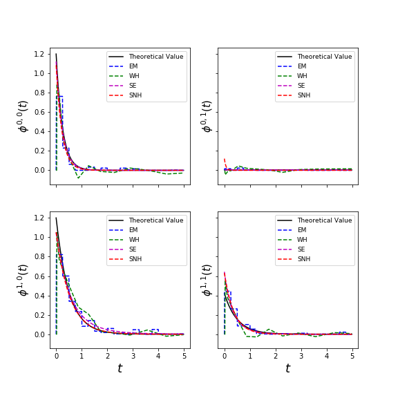


(a) The estimated Exponential kernels (b) The estimated error for Exponential kernels (c) The estimated Power Law kernels (d) The estimated error for Power Law kernels (e) The convergence plot of Negative Log-likelihood for Exponential kernels estimation in SNH model (f) The convergence plot of Negative Log-likelihood for Power Law kernels estimation in SNH model
B.3 K-fold cross validation of real data
Cross-validation is one of the most widely used method for evaluating learning algorithms. Ideally, we divide the dataset into training set, cross-validation set and test set, to optimize the parameters, evaluate each algorithm and finally test the successful algorithm with least error. However, when the data is scarce or limited we are left with fewer numbers of samples in the training set. As a solution to this problem, we use the k-fold cross validation method Friedman et al. 2001 to test the performance of our model. In this method, we divide the dataset into k-groups and for each of these groups we split the training and test set to evaluate the score. The performance measure is the average of the evaluated scores of the k-groups, given as,
| (19) |
For the dataset in our experiment, we use the TimeSeriesSplit function provided by Scikit-learn Pedregosa et al. 2011. Unlike non-time series data where the data are randomly split, this function divides the dataset along with the sequence and successive training sets are supersets of those that come before them. Due to the dependence on history in Hawkes processes, we modify the split function in order to evaluate the negative log-likelihood collectively on training and test samples (rather than on just test samples). The figure 5 demonstrates the time-series cross-validation split on bivariate Bitcoin data, for K = 5 groups. Training sets are of sizes () and their corresponding test sets are of sizes () . The estimated score, i.e the negative log-likelihood values for SNH, EM and WH models are , and respectively.

B.4 Additional analysis on synthetic data
We extend the analysis on univariate Hawkes process described in Section 5.1.1 to study the effect of hyper-parameter choices for SNH. We first study the impact on the performance of SNH model with varied number of neurons. The figure 6 shows the estimated negative log-likelihood values with increasing number of neurons used in the SNH for the exponential form of kernel. We find, as would be expected, that fewer number of neurons are sufficient to achieve convergence. Next, we perform similar analysis on the rectangular kernel described in 5.1.1 and the results are demonstrated in Figure 6. In this case, it is evident that optimum performance is achieved by using neurons in range in the SNH architecture.


(a) The case of exponential kernels (b) The case of rectangular kernels
Next, we investigate the performance of the SNH model based on different choices of learning rates using the rectangular kernel described in 5.1.1, for a fixed number of epochs. We find that using higher learning rates for the outer layer in comparison to the inner layer helps in faster convergence of the results.
| Lr of outer layer | Neg loglik |
|---|---|
| 0.0001 | 37113.09 |
| 0.005 | 20244.66 |
| 0.001 | 20562.68 |
| 0.05 | 20765.67 |
| 0.01 | 20201.20 |
| Lr of inner layer | Neg loglik |
|---|---|
| 0.00001 | 21369.25 |
| 0.00005 | 20483.83 |
| 0.0005 | 20350.01 |
| 0.0001 | 20321.78 |
| 0.005 | 20587.84 |
| 0.01 | 22346.72 |