Flexible Bayesian Modelling
for Nonlinear Image Registration

Mikael Brudfors (✉) Affiliation: Wellcome Centre for Human Neuroimaging, UCL, UK E-mail mikael.brudfors.15@ucl.ac.uk Yaël Balbastre Affiliation: Wellcome Centre for Human Neuroimaging, UCL, UK E-mail mikael.brudfors.15@ucl.ac.uk Guillaume Flandin Affiliation: Wellcome Centre for Human Neuroimaging, UCL, UK E-mail mikael.brudfors.15@ucl.ac.uk Parashkev Nachev Affiliation: UCL Institute of Neurology, UK
* These authors contributed equally to this work John Ashburner Affiliation: Wellcome Centre for Human Neuroimaging, UCL, UK E-mail mikael.brudfors.15@ucl.ac.uk

Abstract

We describe a diffeomorphic registration algorithm that allows groups of images to be accurately aligned to a common space, which we intend to incorporate into the SPM software. The idea is to perform inference in a probabilistic graphical model that accounts for variability in both shape and appearance. The resulting framework is general and entirely unsupervised. The model is evaluated at inter-subject registration of 3D human brain scans. Here, the main modeling assumption is that individual anatomies can be generated by deforming a latent ‘average’ brain. The method is agnostic to imaging modality and can be applied with no prior processing. We evaluate the algorithm using freely available, manually labelled datasets. In this validation we achieve state-of-the-art results, within reasonable runtimes, against previous state-of-the-art widely used, inter-subject registration algorithms. On the unprocessed dataset, the increase in overlap score is over 17%. These results demonstrate the benefits of using informative computational anatomy frameworks for nonlinear registration.

1 Introduction

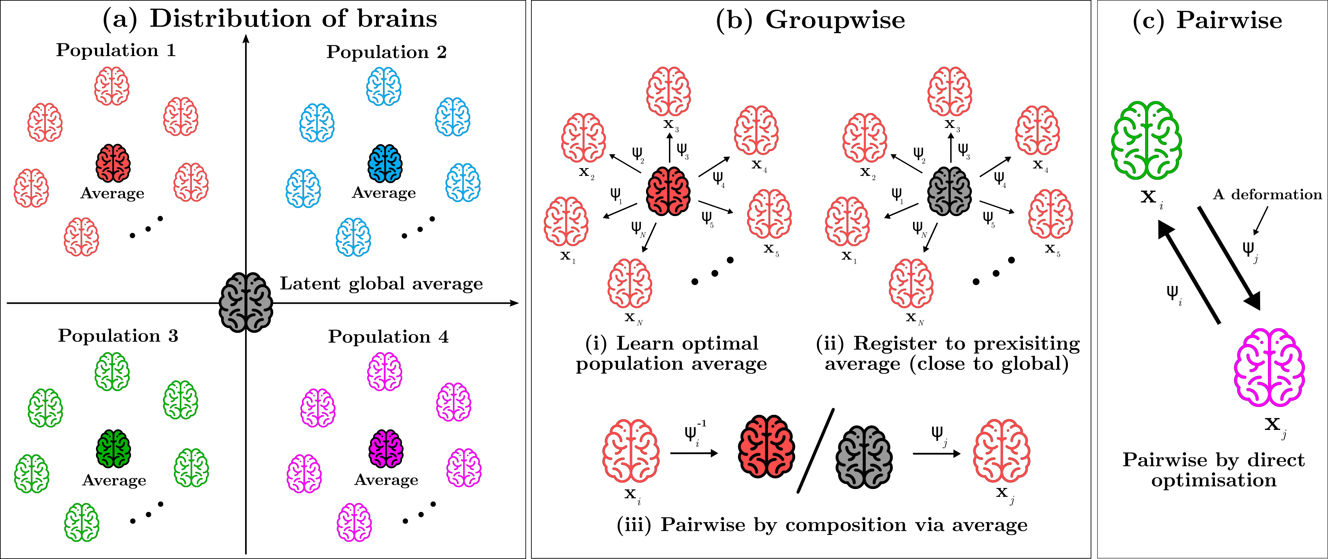
This paper presents a flexible framework for registration of a population of images into a common space, a procedure known as spatial normalisation [1], or congealing [2]. Depending on the quality of the common space, accurate pairwise alignments can be produced by composing deformations that map two subjects to this space. The method is defined by a joint probability distribution that describes how the observed data can be generated. This generative model accounts for both shape and appearance variability; its conditional dependences producing a more robust procedure. Shape is encoded by a tissue template, that is deformed towards each image by a subject-specific composition of a rigid and a diffeomorphic transform. Performing registration on the tissue level, rather than intensity, has been shown to be a more robust method of registering medical images [3]. Appearance is encoded by subject-specific Gaussian mixture models, with prior hyper-parameters shared across the population. A key assumption of the model is that there exists a latent average representation (e.g., brain), this is illustrated in Fig. 1a.

Refer to caption — Figure 1: (a) Multiple populations of brain scans have their individual averages; the assumption in this paper is that there exists a latent global average. (b) A groupwise method can either learn the optimal population-specific average (i), or use an already learned average (ii), the closer the learned average is to the global, the better the method should generalise to unseen test data. In both cases, all population scans are deformed towards the average. Pairwise deformations are then obtained by composing deformations via this average (iii). The proposed approach belongs here, and can be used for both (i) and (ii). (c) A pairwise method directly deforms one image towards another, usually by optimising some similarity metric or by applying a learned function. The common space then consists of just the two images to be registered.

Images of human organs differ in their morphology, the goal of spatial normalisation is to deform individual organs so that anatomical locations correspond between different subjects (a selective removal of the inter-individual anatomical variance). The deformations that are computed from this inter-subject registration therefore capture meaningful individual shape information. Although not constrained to a specific organ, our method will here be applied to spatially normalise brain magnetic resonance images (MRIs). Spatial normalisation is a critical first step in many neuroimaging analyses, e.g., the comparison of tissue composition [4] or functional MRI activation [5] across individuals; shape mapping [6]; the extraction of predictive features for machine learning tasks [7]; or the identification of lesions [8]. The success of these tasks is therefore fundamentally coupled with the quality of the inter-individual alignment. Neuroimaging meta-analysis [9] is another research area that relies on spatial normalisation. Currently, statistical maps are coarsely registered into the MNI space. Better normalisation towards a more generic, multi-modal, high-resolution space could greatly improve the power and spatial specificity of such meta-analyses.

In general, registration tasks can be classified as either pairwise or groupwise (Fig. 1b-c). Pairwise methods optimise a mapping between two images, and only their two spaces exist. Groupwise methods aim to align several images into an optimal common space. Spatial normalisation aims to register a group of images into a pre-existing common space, defined by some average. Most nonlinear registration methods optimise an energy that comprises two terms: one that measures the similarity between a deformed and a fixed image and one that enforces the smoothness of the deformation. Two main families emerge, whether they penalise the displacement fields (inspired by solid physics) or their infinitesimal rate of change (inspired by fluid physics), allowing for large diffeomorphic deformations [10, 11]. Concerning the optimisation scheme, a common strategy is to work with energies that allow for a probabilistic interpretation [12, 13, 14, 15, 16]. The optimisation can in this case be cast as an inference problem, which is the approach taken in this paper. More recently, it has been proposed to use deep neural networks to learn the normalisation function [17, 18, 19, 20]. At training time, however, these approaches still use a two-term loss function that enforces data consistency while penalising non-smoothness of the deformations. These models have demonstrated remarkable speed-ups in runtime for volumetric image registration, with similar accuracies to the more classical methods.

Note that all of the above methods either require some sort of prior image processing or are restricted to a specific MR contrast. The method presented in this paper is instead agnostic to the imaging modality and can be applied directly to the raw data. This is because it models many features of the imaging process (bias field, gridding, etc.), in order not to require any processing such as skull-stripping, intensity normalisation, affine alignment or reslicing to a common grid. These properties are important for a general tool that should work ‘out-of-the-box’, given that imaging protocols are far from standardised – restricting a method to a particular intensity profile considerably restricts its practical use. In addition, our method allows for a user to chose the resolution of the common space. We validate our approach on a pairwise registration task, comparing it against state-of-the-art methods, on publicly available data. We achieve favourable results outperforming all other methods, within reasonable runtimes.

Appearance ( $\mathcal{A}$ )
Intensity:	${\bf f}_{ni}\sim\prod_{k}\mathcal{N}_{C}\left({\bf B}_{ni}^{-1}\bm{\mu}_{k},\left({\bf B}_{ni}\bm{\Lambda}_{k}{\bf B}_{ni}\right)^{-1}\right)^{z_{nik}}$
INU coefficients:	$\bm{\beta}_{nc}\sim\mathcal{N}_{M}\left(\bm{0},\bm{\Lambda}_{\beta}\right)$
Intensity mean:	$\bm{\mu}_{k}\sim\mathcal{N}_{C}\left({\bf m}_{0k},(\beta_{0k}\bm{\Lambda}_{k})^{-1}\right)$
Intensity precision:	$\bm{\Lambda}_{k}\sim\mathcal{W}_{C}\left({\bf W}_{0k},\nu_{0k}\right)$
INU function:	${\bf B}_{ni}=\text{diag}({\bf b}_{ni}),\;{\bf b}_{ni}=\exp\left(\bm{\Upsilon}_{i}\bm{\beta}_{n}\right)$
Intensity parameters:	${\bf m}_{0k},\beta_{0k},{\bf W}_{0k},\nu_{0k}$
Hyper-parameters:	$\bm{\Lambda}_{\beta}\text{ (bending energy)}$
Shape ( $\mathcal{S}$ )
Tissue:	${\bf z}_{ni}\sim\text{Cat}_{K+1}\left(\bm{\pi}_{ni}\right)$
Log-template:	${\bf t}_{k}\sim\mathcal{N}_{I}\left(\bm{0},\bm{\Lambda}_{\text{t}}\right)$
Velocity:	${\bf v}_{n}\sim\mathcal{N}_{I}\left(\bm{0},\bm{\Lambda}_{\text{v}}\right),\;\sum_{n}{\bf v}_{n}=\bm{0}$
Tissue prior:	$\bm{\pi}_{n}=\mathrm{softmax}\left({\bf t}\circ\bm{\psi}_{n}\right)$
Forward deformation:	$\bm{\psi}_{n}=\bm{\phi}({\bf v}_{n})\circ{\bf M}_{\text{t}}{\bf R}({\bf q}_{n}){\bf M}_{n}^{-1}$
Rigid parameters:	${\bf q}_{n},\;\sum_{n}{\bf q}_{n}=\bm{0}$
Hyper-parameters:	$\bm{\Lambda}_{\text{v}}$ , $\bm{\Lambda}_{\text{t}}$ (combination of energies)

Number of
subjects:	$N$ ,	channels:	$C$
subject voxels:	$I_{n}$ ,	bias bases:	$M$
template voxels:	$I$	template classes:	$K$

2 Methods

Generative Model. In this work, computing the nonlinearly aligned images is actually a by-product of doing inference on a joint probability distribution. This generative model consists of multiple random variables, modelling various properties of the observed data. It is defined by the following distribution:

\displaystyle p(\mathcal{F},\mathcal{A},\mathcal{S})=p(\mathcal{F}\mid\mathcal{A},\mathcal{S})~p(\mathcal{A},\mathcal{S}),

(1)

where $\mathcal{F}=\{{\bf F}_{n}\}_{n=1}^{N}$ , ${\bf F}_{n}\in\mathbb{R}^{I_{n}\times C}$ are the $N$ observed images (e.g., MRI scans), each with $I_{n}$ voxels and $C$ channels (e.g., MR contrasts). The two sets $\mathcal{A}$ and $\mathcal{S}$ contain the appearance and shape variables, respectively. The distribution in (1) is unwrapped in detail in Fig. 2, showing its graphical model and constituent parts. The inversion of the model in (1) is performed using a variational expectation-maximisation (VEM) algorithm. In this algorithm, each parameter (or its probability distribution, in the case of the mixture parameters) is updated whilst holding all others fixed, in an alternating manner [22]. The individual update equations are obtained from the evidence lower bound (ELBO):

\displaystyle\mathcal{L}=\sum_{\mathcal{A},\mathcal{S}}q(\mathcal{A},\mathcal{S})\ln\left[\frac{p(\mathcal{F},\mathcal{A},\mathcal{S})}{q(\mathcal{A},\mathcal{S})}\right],

(2)

where the variational distribution is assumed to factorise as $q(\mathcal{A},\mathcal{S})=q(\mathcal{A})q(\mathcal{S})$ . The appearance updates have been published in previous work: the inference of the intensity parameters in [23]; the mode estimates of the intensity non-uniformity (INU) parameters in [12].

The contribution of this paper is to unify the shape and appearance parts as (1), providing a flexible and unsupervised image registration framework. In particular, this framework relies on: parameterising the shape model using a combined rigid and diffeomorphic registration in the space of the template, introduction of a multi-scale optimisation method, and a novel way of computing a Hessian of the categorical data term. These will next be explained in more detail.

Spatial Transformation Model. For maximum generalisability, the model should handle image data defined on arbitrary lattices with arbitrary orientations (i.e., any well formatted NIfTI file). The forward deformation $\vec{\psi}_{n}$ , warping the template to subject space, is the composition of a diffeomorphic transform ${\bm{\phi}}_{n}$ , defined over the template field of view, and a rigid transform ${\bf R}_{n}$ , defined in world space. The template ( ${\bf M}_{\text{t}}$ ) and subject ( ${\bf M}_{n}$ ) orientation matrices describe the mapping from voxel to world space. Therefore, ${\bm{\psi}}_{n}={\bm{\phi}}_{n}\circ{\bf M}_{\text{t}}\circ{\bf R}_{n}\circ{\bf M}_{n}^{-1}$ . The diffeomorphism is encoded by the initial velocity of the template ‘particles’ [24], and recovered by geodesic shooting [25]: ${\bm{\phi}}_{n}=\mathrm{shoot}\left({\bf v}_{n}\right)$ . ${\bf R}_{n}$ is encoded by its projection $\mathbf{q}_{n}$ on the tangent space of rigid transformation matrices, and recovered by matrix exponentiation [26]. ${\bf R}_{n}$ could have included scales and shears, but keeping it rigid allows us to capture these deformations in the velocities.

Multi-Scale Optimisation. Registration is a non-convex problem and is therefore highly sensitive to local minima. Multi-scale optimisation techniques can be used to circumvent this problem [10, 2, 20]. The proposed approach implements such a multi-scale method to help with several difficulties: local minima (especially in the rigid parameter space), slow VEM convergence, and slow runtime. The way we parameterise the spatial transformation model is what enables our multi-scale approach. If we drop all terms that do not depend on the template, velocities or rigid parameters, the ELBO in (2) reduces to:

\displaystyle\mathcal{L}\overset{c}{=}\sum_{n}\Big\{\ln\mathrm{Cat}\left(\tilde{\mathbf{z}}_{n}\mid\mathrm{softmax}\left({\bf t}\circ\bm{\psi}_{n}\right)\right)+\ln p(\vec{v}_{n})\Big\}+\ln p({\bf t})~,

(3)

where $\tilde{\mathbf{z}}_{n}$ denotes the latent class posterior probabilities (responsibilities). The two prior terms originate from the realm of PDEs, where they take the form of integrals of continuous functions. When discretised, these integrals can be interpreted as negative logs of multivariate Normal distributions (up to a constant):

\displaystyle\frac{\lambda}{2}\int_{\Omega}\langle f(\mathbf{x}),(\Lambda f)(\mathbf{x})\rangle d\mathbf{x}\;\xrightarrow{\text{discretise}}\;\frac{\lambda}{2}\left(\mathbf{f}^{\mathrm{T}}\bm{\Lambda}\mathbf{f}\right)~\Delta_{x}.

(4)

Here, $\mathbf{f}^{\mathrm{T}}\bm{\Lambda}\mathbf{f}$ computes the sum-of-squares of the (discrete) image gradients and $\Delta_{x}$ is the volume of one discrete element. Usually, $\Delta_{x}$ would simply be merged into the regularisation factor $\lambda$ . In a multi-scale setting, it must be correctly set at each scale. In practice, the template and velocities are first defined over a very coarse grid, and the VEM scheme is applied with a suitable scaling. At convergence, they are trilinearly interpolated to a finer grid, and the scaling parameter is changed accordingly for a new iteration of VEM.

Böhning Bound. We use a Newton-Raphson algorithm to find mode estimates of the variables $\mathbf{t}$ , $\mathbf{v}_{n}$ and $\mathbf{q}_{n}$ , with high convergence rates. This requires the gradient and Hessian of the categorical data term. If the gradient and Hessian with respect to $\mathbf{t}_{n}={\bf t}\circ\bm{\psi}_{n}$ are known, then those with respect to the variables of interest $\mathbf{t}$ , $\mathbf{v}_{n}$ and $\mathbf{q}_{n}$ can be obtained by application of the chain rule (with Fisher’s scoring [24]). However, the true Hessian is not well-behaved and the Newton-Raphson iterates may overshoot. Therefore, some precautions must be taken such as ensuring monotonicity using a backtracking line search [27]. Here, we make use of Böhning’s approximation [28] to bound the ELBO and improve the stability of the update steps, without the need for line search. This approximation was introduced in the context of multinomial logistic regression, which relies on a similar objective function. Because this approximation allows the true objective function to be bounded, it ensures the sequence of Newton-Raphson steps to be monotically improving. However, this bound is not quite tight, leading to slower convergence rates. In this work, we therefore use a weighted average of Böhning’s approximation and the true Hessian that leads to both fast and stable convergence; e.g., the template Hessian becomes:

\displaystyle\frac{\partial^{2}\mathcal{L}}{\partial t_{nik}\partial t_{nil}}\approx w\underbrace{\pi_{nik}\left(\delta_{k}^{l}-\pi_{nil}\right)}_{\text{True Hessian}}{}+{}(1-w)\underbrace{\frac{1}{2}\left(\delta_{k}^{l}-\frac{1}{K}\right)}_{\text{B\"{o}hning bound}},\quad w\in[0,1].

(5)

3 Validation

Experiments. Brain scans where regions-of-interests have been manually labelled by human experts can be used to assess the accuracy of a registration method. By warping the label images from one subject onto another, overlap scores can be computed, without the need to resample the groundtruth annotations. The labels parcelate the brain into small regions, identifying the same anatomical structures between subjects. As the labels are independent from the signal used to compute the deformations, they are well suited to be used for validation. Such a validation was done in a seminal paper [29], where 14 methods were compared at nonlinearly registering pairs of MR brain scans. Two datasets used in [29] were¹¹ 1 nitrc.org/projects/ibsr, resource.loni.usc.edu/resources:

•

LPBA40: T1-weighted (T1w) MRIs of 40 subjects with cortical and subcortical labels, of which 56 were used in the validation in [29]. The two top-performing methods, from $N=1,560$ pairwise registrations, were ART’s 3dwarper [30] and ANTs’ SyN [11]. The MRIs have been processed by skull-stripping, non-uniformity correction, and rigid reslicing to a common space.
•

IBSR18: T1w MRIs of 18 subjects with cortical labels, where 96 of the labelled regions were used in the validation in [29]. The two top-performing methods, from $N=306$ pairwise registrations, were SPM’s Dartel [13] and ANTs’ SyN [11]. The MRIs have non-isotropic voxels and are unprocessed; IBSR18 are therefore more challenging to register than LPBA40.

We now compare our method, denoted MultiBrain (MB), with the top-performing methods in [29], on IBSR18 and LPBA40. The same overlap metric is used: the volume over which the deformed source labels match the target labels, divided by the total volume of the target labels (i.e., the true positive rate (TPR)). Two additional registration methods are included: one state-of-the-art group-wise model, SPM’s Shoot [31]; and one state-of-the-art deep learning model, the CVPR version of VoxelMorph²² 2 github.com/voxelmorph/voxelmorph (VXM) [17]. Pairwise registrations between all subjects (in both directions) are computed using MB, SPM’s Shoot and VXM. For MB, we (i) learned the optimal average from each dataset (MB-GW), and (ii) learned the optimal average from a held-out training set (MB-L); as described in Fig. 1b. These two tasks are similar to either finding the optimal template for a specific neuroimaging group study (MB-GW) or using a predefined common space for the same task (MB-L). Shoot’s registration process resembles MB-GW, whilst VXM resembles MB-L. MB-L was trained on $N=277$ held-out T1w MRIs from five different datasets: three publicly available³³ 3 brain-development.org, mrbrains18.isi.uu.nl, my.vanderbilt.edu/masi: IXI ( $N_{1}=200$ ), MICCAI2012 ( $N_{2}=35$ ) and MRBrainS18 ( $N_{3}=7$ ); and two hospital curated ( $N_{4}=19$ , $N_{5}=16$ ). Training took two days on a modern workstation.

The shape and appearance models that were learned when fitting MB are shown in Fig. 3. $K=11$ classes were used, 1 mm isotropic template voxels and the priors were initialised as uninformative. The initial template and velocity dimensions were set to 8 mm cube. Energy hyper-parameters were chosen as $\lambda_{\beta}=1\text{e}5$ , $\lambda_{\text{v}}=\{2\text{e-}4,0,0.4,0.1,0.4\}$ (absolute, membrane, bending, linear elasticity) and $\lambda_{\text{t}}=\{1\text{e-}2,0.5,0\}$ (absolute, membrane, bending). The weighting was set to $w=0.8$ . The algorithm was run for a predefined number of iterations.

Results. The label overlap scores on IBSR18 are shown in Fig. 4. The figure shows, close to, unanimous better overlap for MB, compared to the other algorithms. Result plots for LPBA40 are given in the supplementary materials, as well as samples of the best and worst registrations for MB and VXM. On both IBSR18 and LPBA40, MB performs favourably. For IBSR18, the mean and median overlaps were 0.62 and 0.63 respectively for MB-GW, and both 0.59 for MB-L. Mean and median overlaps were both 0.59 for SPM’s Shoot and both 0.56 for VXM. The greatest median overlap reported in [29] was about 0.55, whereas the overlap from affine registration was 0.40 [32]. For LPBA40, the mean and median overlaps were both 0.76 for MB-GW and both 0.75 for MB-L. Mean and median overlaps for SPM’s Shoot approach were both 0.75, and both 0.74 for VXM. The highest median overlap reported in [29] was 0.73, and that from affine registration was 0.60 [32]. Using the affine registrations as baseline, the results showed 6% to 17% greater accuracy improvements when compared to those achieved for the second most accurate nonlinear registration algorithm evaluated⁴⁴ 4 $(\text{TPR}_{\mathrm{MB}}-\text{TPR}_{\mathrm{Shoot}})/(\text{TPR}_{\mathrm{MB}}-\text{TPR}_{\mathrm{Affine}})\times 100\%$ . Computing one forward deformation took about 15 minutes for MB-L and 30 for MB-GW (on a modern workstation, running on the CPU).

Discussion. MB-GW does better than MB-L, this was expected as the average obtained by groupwise fitting directly on the population of interest should be more optimal than one learned from a held-out dataset, on a limited number of subjects (e.g., the averages for the individual populations in Fig. 1 are more optimal than the global). Still, MB-L learned on only 277 subject does as well as, or better than, Shoot (a state-of-the-art groupwise approach). This is an exciting result that allows for groupwise accuracy spatial normalisation on small number of subjects, and to a standard common space (instead of a population-specific). With a larger and more diverse training population, accuracies are expected to improve further. One may claim that a group-wise registration scheme has unfair advantage over pairwise methods. However, as a common aim often is to spatially normalise - with the objective of making comparisons among a population of scans, it would be reasonable to aim for as much accuracy as possible for this task. The purely data-driven VXM approach does better than the methods evaluated in [29]. VXM was trained on close to 4,000 diverse T1w MRIs. A larger training dataset could boost its performance. The processing that was applied to the VXM input data was done using SPM [33], whilst its training data was processed using FreeSurfer. Having used the same software could have improved its results; however, being reliant on a specific processing pipeline is inherently a weakness of any method. Furthermore, the VXM model uses a cross-correlation loss function that should be resilient to intensity variations in the T1w scans. Finally, the contrasts and fields of view in the T1w scans were slightly different from each other in the training and testing data, due to variability in field strength and scanner settings. This could have impacted the accuracy of MB-L and VXM.

4 Conclusion

This paper introduced an unsupervised learning algorithm for nonlinear image registration, which can be applied to unprocessed medical imaging data. A validation on two publicly available datasets showed state-of-the art results on registering MRI brain scans. The unsupervised, non-organ specific nature of the algorithm makes it applicable to not only brain data, but also other types of medical images. This could allow for transferring methods widely used in neuroimaging to other types of organs, e.g., the liver [34]. The runtime of the algorithm is not on par with a GPU implementation of a deep learning model, but still allows for processing of a 3D brain scan in an acceptable time. The runtime should furthermore improve, drastically, by an implementation on the GPU. The proposed model could also be used for image segmentation [12] and translation [36], or modified to use labelled data, in a semi-supervised manner [23]. Finally, the multi-modal ability of the model would be an interesting avenue of further research.

Acknowledgements:

MB was funded by the EPSRC-funded UCL Centre for Doctoral Training in Medical Imaging (EP/L016478/1) and the Department of Health’s NIHR-funded Biomedical Research Centre at University College London Hospitals. YB was funded by the MRC and Spinal Research Charity through the ERA-NET Neuron joint call (MR/R000050/1). MB and JA were funded by the EU Human Brain Project’s Grant Agreement No 785907 (SGA2). GF and the Wellcome Centre for Human Neuroimaging is supported by core funding from the Wellcome (203147/Z/16/Z).

References

[1] K. J. Friston, J. Ashburner, C. D. Frith, J.-B. Poline, J. D. Heather, and R. S. Frackowiak, “Spatial registration and normalization of images,” Human brain mapping, vol. 3, no. 3, pp. 165–189, 1995.
[2] L. Zöllei, E. Learned-Miller, E. Grimson, and W. Wells, “Efficient population registration of 3D data,” in CVBIA, pp. 291–301, Springer, 2005.
[3] R. A. Heckemann, S. Keihaninejad, P. Aljabar, D. Rueckert, J. V. Hajnal, A. Hammers, A. D. N. Initiative, et al., “Improving intersubject image registration using tissue-class information benefits robustness and accuracy of multi-atlas based anatomical segmentation,” Neuroimage, vol. 51, no. 1, pp. 221–227, 2010.
[4] B. Draganski, C. Gaser, V. Busch, G. Schuierer, U. Bogdahn, and A. May, “Changes in grey matter induced by training,” Nature, vol. 427, no. 6972, pp. 311–312, 2004.
[5] P. T. Fox, “Spatial normalization origins: Objectives, applications, and alternatives,” Human brain mapping, vol. 3, no. 3, pp. 161–164, 1995.
[6] J. G. Csernansky, S. Joshi, L. Wang, J. W. Haller, M. Gado, J. P. Miller, U. Grenander, and M. I. Miller, “Hippocampal morphometry in schizophrenia by high dimensional brain mapping,” PNAS, vol. 95, no. 19, pp. 11406–11411, 1998.
[7] J. Mourao-Miranda, A. Reinders, V. Rocha-Rego, J. Lappin, J. Rondina, C. Morgan, K. D. Morgan, P. Fearon, P. B. Jones, G. A. Doody, et al., “Individualized prediction of illness course at the first psychotic episode: a support vector machine mri study,” Psychological medicine, vol. 42, no. 5, pp. 1037–1047, 2012.
[8] M. L. Seghier, A. Ramlackhansingh, J. Crinion, A. P. Leff, and C. J. Price, “Lesion identification using unified segmentation-normalisation models and fuzzy clustering,” NeuroImage, vol. 41, no. 4, pp. 1253–1266, 2008.
[9] T. Yarkoni, R. A. Poldrack, T. E. Nichols, D. C. Van Essen, and T. D. Wager, “Large-scale automated synthesis of human functional neuroimaging data,” Nature methods, vol. 8, no. 8, p. 665, 2011.
[10] G. E. Christensen, S. C. Joshi, and M. I. Miller, “Volumetric transformation of brain anatomy,” IEEE transactions on medical imaging, vol. 16, no. 6, pp. 864–877, 1997.
[11] B. B. Avants, C. L. Epstein, M. Grossman, and J. C. Gee, “Symmetric diffeomorphic image registration with cross-correlation: evaluating automated labeling of elderly and neurodegenerative brain,” Medical image analysis, vol. 12, no. 1, pp. 26–41, 2008.
[12] J. Ashburner and K. J. Friston, “Unified segmentation,” NeuroImage, vol. 26, no. 3, pp. 839–851, 2005.
[13] J. Ashburner, “A fast diffeomorphic image registration algorithm,” NeuroImage, vol. 38, no. 1, pp. 95–113, 2007.
[14] J. L. Andersson, M. Jenkinson, S. Smith, et al., “Non-linear registration aka spatial normalisation FMRIB technial report TR07JA2,” FMRIB Analysis Group of the University of Oxford, 2007.
[15] K. K. Bhatia, P. Aljabar, J. P. Boardman, L. Srinivasan, M. Murgasova, S. J. Counsell, M. A. Rutherford, J. V. Hajnal, A. D. Edwards, and D. Rueckert, “Groupwise combined segmentation and registration for atlas construction,” in MICCAI, pp. 532–540, Springer, 2007.
[16] T. Vercauteren, X. Pennec, A. Perchant, and N. Ayache, “Diffeomorphic demons: Efficient non-parametric image registration,” NeuroImage, vol. 45, no. 1, pp. S61–S72, 2009.
[17] G. Balakrishnan, A. Zhao, M. R. Sabuncu, J. Guttag, and A. V. Dalca, “VoxelMorph: a learning framework for deformable medical image registration,” IEEE transactions on medical imaging, vol. 38, no. 8, pp. 1788–1800, 2019.
[18] A. Dalca, M. Rakic, J. Guttag, and M. Sabuncu, “Learning conditional deformable templates with convolutional networks,” in NeurIPS, pp. 804–816, 2019.
[19] J. Fan, X. Cao, P.-T. Yap, and D. Shen, “BIRNet: Brain image registration using dual-supervised fully convolutional networks,” Medical image analysis, vol. 54, pp. 193–206, 2019.
[20] J. Krebs, H. Delingette, B. Mailhé, N. Ayache, and T. Mansi, “Learning a probabilistic model for diffeomorphic registration,” IEEE transactions on medical imaging, vol. 38, no. 9, pp. 2165–2176, 2019.
[21] M. F. Beg and A. Khan, “Computing an average anatomical atlas using LDDMM and geodesic shooting,” in ISBI, pp. 1116–1119, IEEE, 2006.
[22] C. M. Bishop, Pattern Recognition and Machine Learning. Springer, 2006.
[23] C. Blaiotta, P. Freund, M. J. Cardoso, and J. Ashburner, “Generative diffeomorphic modelling of large mri data sets for probabilistic template construction,” NeuroImage, vol. 166, pp. 117–134, 2018.
[24] J. Ashburner, M. Brudfors, K. Bronik, and Y. Balbastre, “An algorithm for learning shape and appearance models without annotations,” Medical image analysis, vol. 55, p. 197, 2019.
[25] M. I. Miller, A. Trouvé, and L. Younes, “Geodesic shooting for computational anatomy,” Journal of mathematical imaging and vision, vol. 24, no. 2, pp. 209–228, 2006.
[26] R. P. Woods, “Characterizing volume and surface deformations in an atlas framework: theory, applications, and implementation,” NeuroImage, vol. 18, no. 3, pp. 769–788, 2003.
[27] J. Ashburner and K. J. Friston, “Computing average shaped tissue probability templates,” NeuroImage, vol. 45, no. 2, pp. 333–341, 2009.
[28] D. Böhning, “Multinomial logistic regression algorithm,” Annals of the institute of Statistical Mathematics, vol. 44, no. 1, pp. 197–200, 1992.
[29] A. Klein, J. Andersson, B. A. Ardekani, J. Ashburner, B. Avants, M.-C. Chiang, G. E. Christensen, D. L. Collins, J. Gee, P. Hellier, et al., “Evaluation of 14 nonlinear deformation algorithms applied to human brain MRI registration,” NeuroImage, vol. 46, no. 3, pp. 786–802, 2009.
[30] B. A. Ardekani, S. Guckemus, A. Bachman, M. J. Hoptman, M. Wojtaszek, and J. Nierenberg, “Quantitative comparison of algorithms for inter-subject registration of 3D volumetric brain MRI scans,” Journal of neuroscience methods, vol. 142, no. 1, pp. 67–76, 2005.
[31] J. Ashburner and K. J. Friston, “Diffeomorphic registration using geodesic shooting and gauss–newton optimisation,” NeuroImage, vol. 55, no. 3, pp. 954–967, 2011.
[32] M. Jenkinson, P. Bannister, M. Brady, and S. Smith, “Improved optimization for the robust and accurate linear registration and motion correction of brain images,” NeuroImage, vol. 17, no. 2, pp. 825–841, 2002.
[33] I. B. Malone, K. K. Leung, S. Clegg, J. Barnes, J. L. Whitwell, J. Ashburner, N. C. Fox, and G. R. Ridgway, “Accurate automatic estimation of total intracranial volume: a nuisance variable with less nuisance,” NeuroImage, vol. 104, pp. 366–372, 2015.
[34] G. Ridgway, K. Janowski, A. Dennis, V. Bachtiar, J. McGonigle, C. Everitt, A. Darekar, D. Breen, D. Green, S. Neubauer, et al., “Voxel-wise analysis of paediatric liver MRI,” in MIUA, pp. 57–62, Springer, 2018.
[35] C. L. Richardson and L. Younes, “Metamorphosis of images in reproducing kernel Hilbert spaces,” Advances in Computational Mathematics, vol. 42, no. 3, pp. 573–603, 2016.
[36] M. Brudfors, J. Ashburner, P. Nachev, and Y. Balbastre, “Empirical Bayesian mixture models for medical image translation,” in SASHIMI, pp. 1–12, Springer, 2019.

Flexible Bayesian Modelling for Nonlinear Image Registration