PolyDL: Polyhedral Optimizations for Creation of High Performance DL primitives

Sanket Tavarageri, Alexander Heinecke, Sasikanth Avancha, Bharat Kaul Affiliation: Intel Labs email: sanket.tavarageri@intel.com and Gagandeep Goyal, Ramakrishna Upadrasta Affiliation: IIT Hyderabad email: ramakrishna@iith.ac.in

Abstract.

Deep Neural Networks (DNNs) have revolutionized many aspects of our lives. The use of DNNs is becoming ubiquitous including in software for image recognition, speech recognition, speech synthesis, language translation, to name a few. The training of DNN architectures however is computationally expensive. Once the model is created, its use in the intended application – the inference task, is computationally heavy too and the inference needs to be fast for real time use. For obtaining high performance today, the code of Deep Learning (DL) primitives optimized for specific architectures by expert programmers exposed via libraries is the norm. However, given the constant emergence of new DNN architectures, creating hand optimized code is expensive, slow and is not scalable.

To address this performance-productivity challenge, in this paper we present compiler algorithms to automatically generate high performance implementations of DL primitives that closely match the performance of hand optimized libraries. We develop novel data reuse analysis algorithms using the polyhedral model to derive efficient execution schedules automatically. In addition, because most DL primitives use some variant of matrix multiplication at their core, we develop a flexible framework where it is possible to plug in library implementations of the same in lieu of a subset of the loops. We show that such a hybrid compiler plus a minimal library-use approach results in state-of-the-art performance. We develop compiler algorithms to also perform operator fusions that reduce data movement through the memory hierarchy of the computer system. Using Convolution Neural Network (CNN) models and matrix multiplication operations, we demonstrate that our approach automatically creates high performing DNN building blocks whose performance matches the performance of hand-crafted kernels of Intel’s oneDNN library on high end CPUs. At the same time, our techniques take only a fraction of time ( $\frac{1}{20}$ or less) compared to AutoTVM, a deep learning auto-tuner to create optimized implementations.

1. Introduction

Deep learning has revolutionized many spheres of human activity, examples of which include, speech recognition (Hinton et al. 2012), image recognition (Krizhevsky et al. 2012; He et al. 2016), web search (goo [n.d.]), language translation (Wu et al. 2016), conversational artificial intelligence (Devlin et al. 2018) etc. Training and inference using deep neural networks (DNNs) that lie at the heart of Deep Learning (DL) are computationally intensive tasks. In today’s datacenters, predominantly CPUs are used for inference tasks partly due to latency considerations. According to a recent McKinsey study (Batra et al. 2018), CPUs account for 75% of the inference market. Software frameworks such as TensorFlow, and PyTorch have been created to allow data scientists to write high performance deep learning code in an efficient manner. However, all these frameworks use manually optimized primitives to deliver high performance.

Given the ubiquity of CPUs and their widespread use for inference in deep learning applications, in this work we focus on automatically creating high performance implementations of DL primitives on CPU platforms. Creating a high performance implementation of a DL primitive requires that the code is parallelized in a load balanced fashion to take advantage of the multiple cores. Within a single core, the code should be cache friendly: this often means the loops of the code are tiled so that effective data reuse out of different levels of cache (L1, L2, and L3) is possible. Tiling/blocking program transformation (Bondhugula et al. 2008) facilitates data reuse from caches and therefore masks the long latency of fetching data from the main memory. Additionally, CPUs feature wide SIMD/vector units. Therefore, the loops should be adequately vectorized. Oftentimes, the different transformations mentioned are intertwined and that presents challenges for the compiler to produce fully optimized code automatically. Existing automatic compilation, and auto-tuning techniques (Bondhugula et al. 2008; Kong and Pouchet 2019; Tavarageri et al. 2013; Renganarayanan et al. 2007; Darte et al. 2014; Baskaran et al. 2010; Hartono et al. 2009; Tavarageri et al. 2010; Chen et al. 2018b; Baghdadi et al. 2019; Chung et al. 2004; Chen 2007; Tiwari et al. 2009) are either 1) inadequate to generate code that matches the performance of hand-tuned library implementations – later on in the paper we show that the state-of-the-art compiler generated code can lag library implementations by as much as ~10X or more, or 2) expensive – it would require running of 1000s of code versions to discover the best performing version and yet, fall short of reaching the peak performance of the machine. The main reason for the failure of automatic compilation techniques in achieving very high performance levels needed is that the sophistication in the CPU microarchitecture has increased over successive generations of CPUs (data prefetching, speculative execution, vector units, deep memory hierarchies, complex cache replacement algorithms etc). Consequently, the cost functions used to optimize code are unable to capture the nitty-gritties of the underlying architectures, and therefore are unable to derive the most effective execution schedules. Auto-tuning is an alternative approach where one explores a large number of program variants and selects the best performing version, sidestepping the complexity of defining a cost function that adequately models the intricacies of the underlying hardware architecture. However, auto-tuning is expensive and furthermore, it may fall short of manually created library in performance as our study shows later on in the paper with respect to AutoTVM (Chen et al. 2018b), a deep learning auto-tuning system. We characterize the performance, productivity trade-off qualitatively in Figure 1.

At the one end of the spectrum, expert coded primitives such as that of Intel oneDNN library attain high performance at the cost of productivity – expert programmers have to hand craft the logic of the primitives for the target architectures. Autotuning systems ease the burden on programming to an extent but do not attain highest levels of performance. Using functionally correct code with vendor supplied compilers is most productive but comes at the expense of performance. Our work – PolyDL is close to attaining the highest levels of performance and at the same time being most productive.

Figure 1. The performance, productivity trade-off of different approaches

It has been shown that 95% of all deep learning applications running in the data centers today have a recurring pattern in their inner most loops, namely blocked matrix multiplication (Jouppi et al. 2017; Georganas et al. 2020). We decompose the overall DL primitive optimization problem into two parts: 1) efficient parallelization of the code and discovering a structure of the loops that uses the multi-level caches well, and 2) effective vectorization of the code for a high degree utilization of the vector units. In this paper, we develop a novel polyhedral model based data reuse algorithm to derive load balanced parallel loops and cache friendly execution schedules. For the latter i.e., to use the vector units optimally, we develop a flexible framework where the inner most loops of kernels can be replaced with microkernels, i.e., manually optimized library implementations. As the number of recurring patterns in the inner most loops of DL primitives is small, our hybrid approach is more scalable because the number of microkernels that the expert programmers have to create is small as well. Thus, the problem of DL library development will now be reduced to hand coding a few microkernels as opposed to hand coding each of the large number of DL primitives.

To account for the sophisticated memory hierarchy, we use a code-generator to create a number of program variants - $n$ in number - for a given program. The generated code variants are then analyzed by our novel data reuse algorithm – PolyDL to characterize their cache behavior. We have developed a relative ranking algorithm which ranks the $n$ variants based on their potential performance. The top $k$ variants are selected and are run on the target hardware and the best performing program version is discovered. Thus, PolyDL narrows down the number of variants to actually run on the target architecture from $n$ to a small, manageable $k$ ( $k<<n$ ). Through our experimental evaluation on convolutions of a range of popular and the state-of-the-art image recognition models, we show that the top variant (a single variant) picked by our compilation machinery is one of the best performing variants, and the realized performance is close to and in many cases, higher than that of Intel’s oneDNN library (int [n.d.]) (formerly known as MKL-DNN), a hand-tuned library for deep learning kernels. Additionally, we develop a fusion algorithm that “fuses” element-wise operators with their preceding or succeeding compute-intensive operators. Such patterns where a computationally heavy operator such as convolution is succeeded by element-wise operators such as ReLU, occur frequently in DL workloads. Therefore, the DL domain specific fusion algorithm that we develop will increase the overall performance by reducing the extra memory traffic that the element-wise operators would otherwise incur.

The contributions of the paper are the following:

•

We present a novel cache data reuse analysis to characterize a loop nest’s behavior with respect to a multi-level cache hierarchy.
•

We describe a methodology to rank program variants in terms of performance using the compiler generated statistics and the system parameters, i.e., cache sizes. To this purpose, we develop two ranking techniques: one, a heuristic for ranking and two, a DNN based approach.
•

We develop a deep learning domain specific operator fusion algorithm.
•

We conduct extensive experiments comparing our technology with the Intel oneDNN library and with AutoTVM. The experiments show that we are able to match the performance of expert coded DL primitives in the oneDNN library and exceed the performance of the ones discovered by AutoTVM via extensive auto-tuning.

To the best of our knowledge, this is the first work that examines automatic compilation techniques and the use of microkernels in an integrated fashion. The rest of the paper is organized as follows. We motivate the need for derivation of automatic execution schedules for loops in Section 2. Section 3 describes preliminary concepts that will be used in developing the compiler algorithms. In Section 4, we develop algorithms for compile-time selection of top performing code version(s). We present a cache data reuse analysis and a poly-ranking system to rank the candidate program variants in terms of performance. The operator fusion algorithm is expounded in Section 5. Section 6 details the experimental evaluation conducted. The related work is discussed in Section 7 while Section 8 presents the conclusions from this work.

2. Motivation

The deep learning primitives are computationally intensive and most of the neural network training and inferencing time is spent in them. However, for different layers of the deep neural networks, the optimizations (e.g., loop order, tile sizes in tiled code etc) that need to be applied are different. Using a version of the code optimized for one layer of a neural network for all others can yield poor performance for the overall neural network. It is this need for custom optimization for different layers of neural networks (the number of layers in a deep neural network can be large) that makes generating efficient code for deep learning primitives a challenging problem. To illustrate the need for such tailored loop optimizations we consider the convolution layers of the Fast R-CNN model (Girshick 2015), one of the leading image recognition CNN models. We generate four variants of convolution code which differ only in the loop order and the rest of the loop structure remains the same for all of them (more details are provided in §6) and measure performance on a 28-core Intel(R) Xeon(R) Platinum 8280 (a.k.a Cascade Lake) CPU server. Figure 3 shows the normalized performance of the code variants on 25 convolution layers of Fast R-CNN: the performance is normalized with respect to the highest performing code among the four variants.

Refer to caption — Figure 2. Performance of four code variants

From Figure 3, we observe that the performances of different versions of the code vary widely from layer to layer. A convolution layer differs from another convolution layer in problem sizes – image sizes, channel widths, filter sizes, strides, and padding. The code version v2 has the best performance from layer 1 through 19, and is subpar from layer 20 through 25. The efficiencies of the other versions viz., v1, v3, and v4 are much more widely varying. Using the compiler technology we have developed – PolyDL that we detail in the rest of the paper, we are able to effectively analyze the four code variants and pick the best performing variant for each layer. The performance achieved by PolyDL picked code shown in Figure 3 is close to the highest performance among the four variants for all 25 layers of Fast R-CNN. Thus using the PolyDL system, using compile-time static analysis alone, we are able to automatically identify and apply the loop optimizations required for each layer of a deep neural network in order to achieve high performance.

3. Preliminaries

3.1. Notation

We use the polyhedral model (Feautrier 1996), which is an advanced mathematical framework to reason about dependences and loop transformations, to develop our data reuse algorithm. We use the Integer Set Library (Verdoolaege 2010) for performing polyhedral operations in this work and we use the same notation as used in ISL to elucidate the concepts and the algorithm. The matrix multiplication code shown in Figure 4 will be used to illustrate the workings of the data reuse analysis.

⬇

for (i = 0; i < M; i++) {

for (j = 0; j < N; j++) {

for (k = 0; k < K; k++) {

C[i][j] += A[i][k] * B[k][j];

}

Figure 4. Matrix multiplication code

Sets

A set is a tuple of variables $x_{i}$ s along with a collection of constraints $c_{k}$ s defined on the tuple variables. $s=\{[x_{1},\dots,x_{n}]:c_{1}\land\dots c_{m}\}$

The iteration spaces of loop nests are represented by sets. The iteration space of the loop in Figure 4 is defined as the following set. $I=\{S[i,j,k]:0<=i<M\land 0<=j<N\land 0<=k<K\}$

Relations

A relation is a mapping from input tuple variables $x_{i}$ s to output tuple variables $y_{j}$ s. In addition, a set of constraints $c_{k}$ s can be defined for a relation that will place constraints on the input/output tuple variables. $r=\{[x_{1},\dots,x_{n}]\mapsto[y_{1},\dots,y_{m}]:c_{1},\dots,c_{p}\}$

The read and write access functions of a loop nest can be modeled with relations. The read relations in the Figure 4 code are shown below: $r_{1}=\{S[i,j,k]\mapsto C[i,j]\}$ , $r_{2}=\{S[i,j,k]\mapsto A[i,k]\}$ , $r_{3}=\{S[i,j,k]\mapsto B[k,j]\}$ . The sole write relation in the loop is: $w_{1}=S[i,j,k]\mapsto C[i,j]$ . The domain of a relation $r$ is denoted by dom $r$ .

Apply operation

When a relation $r$ is applied on a set $s$ , the domain of $r$ will be intersected with $s$ and the resulting range will be a new set $s^{\prime}$ . The set $s^{\prime}$ is said to be the result of the apply operation. The operation is mathematically defined as: $(\vec{y}\in s^{\prime})\Longleftrightarrow(\exists\vec{x}~~\text{s.t}~~(\vec{x}\in s\land\vec{x}\mapsto\vec{y})\in r)$

The data footprint of the loop can be computed by applying read and write relations on the iteration space set: $r_{1}(I)\cup r_{2}(I)\cup r_{3}(I)\cup w_{1}(I)$

Lexicographic operations

The lexicographical operations can be applied on sets. $s_{1}<<s_{2}$ outputs all the elements of $s_{1}$ that are lexicographically strictly smaller than all the elements of $s_{2}$ , while $s_{1}<<=s_{2}$ gets us the elements of $s_{1}$ that are lexicographically smaller than or equal to the elements of $s_{2}$ . The lexicographically smallest element of a set $s$ is queried using lexmin $s$ . Similarly, the lexicographically largest element is obtained using lexmax $s$ .

Set difference.

The set difference between set $s_{1}$ and $s_{2}$ is denoted by $s_{1}-s_{2}$ , i.e., the resulting set will have elements of $s_{1}$ that do not appear in $s_{2}$ .

3.2. Polyhedral dependences

The exact data dependences in loop nests can be computed in the polyhedral model and are expressed as maps from source iterations to target iterations involved in the dependence. For cache data reuse analysis developed in §4, we consider four kinds of dependences – Read-After-Read (RAR), Read-After-Write (RAW, a.k.a flow), Write-After-Read (WAR, a.k.a anti), and Write-After-Write (WAW). The data dependencies of the matrix multiplication code in Figure 4 are shown below.

	$\displaystyle d_{1}=$	$\displaystyle\{S[i,j,k]\mapsto S[i^{\prime},j^{\prime},k^{\prime}]:i^{\prime}=i\land j^{\prime}=j\land k<k^{\prime}<K\}$
	$\displaystyle d_{2}=$	$\displaystyle\{S[i,j,k]\mapsto S[i^{\prime},j^{\prime},k^{\prime}]:i^{\prime}=i\land k^{\prime}=k\land j<j^{\prime}<N\}$
	$\displaystyle d_{3}=$	$\displaystyle\{S[i,j,k]\mapsto S[i^{\prime},j^{\prime},k^{\prime}]:j^{\prime}=j\land k^{\prime}=k\land i<i^{\prime}<M\}$

The dependence $d_{2}$ is induced by array reference A[i][k]. An element of array A, say A[0][0] which is accessed in source iteration $[i=0,j=0,k=0]$ gets reused in target iterations $[i^{\prime}=0,j^{\prime}>0,k^{\prime}=0]$ . The source to target iteration relationships such as this are expressed in a parametric fashion as the relation $d_{2}$ .

Figure 5. The PolyDL system

4. Compile Time Selection of Top performing code version

The input to our compiler tool is, the loop nest to be optimized – $\mathcal{L}$ along with the microkernel that forms the inner-most loops. Figure 5 shows the overall system design. The loop based specification of the microkernel – $\mathcal{M}$ is substituted in the code for further analysis. The resulting loop structure – $\mathcal{L^{\prime}}$ is regular. The code generator takes the loop nest $\mathcal{L^{\prime}}$ and generates a large number of program variants while keeping the inner most loops that correspond to $\mathcal{M}$ intact. For each generated code variant, the working set sizes are computed as described in §4.1. The statistics calculated for all the variants are then input to the poly-ranking algorithm described in §4.2 and it picks the top $k$ best performing versions. The original microkernels are inserted back into the code of the $k$ picks. The top performing variants selected analytically are now run on the target architecture and best performing code among the $k$ loop nests is determined.

Microkernel Specification The microkernel function call is annotated with a pragma compiler directive which contains the loop-based functionally equivalent code. The microkernel function call is substituted with the loop based code for the compiler analysis in a pre-processing pass. When the cache data reuse analysis and ranking of the code variants are done, in a post-processing pass, the loop-based inner most loops are replaced with the call to the microkernel.

We assume that the data accessed by the microkernel’s equivalent loop based code and by the implementation of the microkernel are the same. The order of the loops within the microkernel implementation could be potentially different. There is no assumption on how the microkernel is implemented. The only assumption is that the data set accessed should be the same.

Input: Loop nest:

\mathcal{L}

Output: The working set sizes:

WS_{\text{all}}

{Iteration space:

\mathcal{I}

, Read relations:

r_{\text{read}}

, Write relations:

r_{\text{write}}

, Schedule:

\delta

}

\leftarrow

Parse the loop nest

\mathcal{L}

{

\mathcal{D}_{\text{RAR}},\mathcal{D}_{\text{RAW}},\mathcal{D}_{\text{WAR}},\mathcal{D}_{\text{WAW}}

}

\leftarrow

Compute read-after-read, read-after-write, write-after-read, write-after-write dependences of

\mathcal{L}

\mathcal{D}_{\text{all}}\leftarrow\mathcal{D}_{\text{RAR}}\cup\mathcal{D}_{\text{RAW}}\cup\mathcal{D}_{\text{WAR}}\cup\mathcal{D}_{\text{WAW}}

WS_{\text{all}}\leftarrow\emptyset

/* Iterate through all dependences to compute the working set sizes */

for $d\in\mathcal{D}_{\text{all}}$ do 1

if $d$ spans parallel iterations then 2

/* The dependence spans iterations of the parallel loop(s) */

i_{p}\leftarrow

The outermost parallel iterator in dom

d

\mathcal{I}_{\text{par}}\leftarrow

Parameterize iterators outer to

i_{p}

\mathcal{I}

WS_{\text{par}}\leftarrow|r_{\text{read}}(\mathcal{I}_{\text{par}})\cup r_{\text{write}}(\mathcal{I}_{\text{par}})|

Add

WS_{\text{par}}

WS_{\text{all}}

else 3

/* The dependence spans iterations of the sequential loops */

\mathcal{I}_{\text{source}}\leftarrow\text{lexmin dom}~~~d

\mathcal{I}_{\text{{min\_tar}}}\leftarrow\text{lexmin}~~~d(\mathcal{I}_{\text{source}})

\mathcal{I}_{\text{max\_tar}}\leftarrow\text{lexmax}~~~d(\mathcal{I}_{\text{source}})

\mathcal{I}_{\text{min\_WS}}\leftarrow(\mathcal{I}<<=\mathcal{I}_{\text{min\_tar}})-(\mathcal{I}<<\mathcal{I}_{\text{source}})

\mathcal{I}_{\text{max\_WS}}\leftarrow(\mathcal{I}<<=\mathcal{I}_{\text{max\_tar}})-(\mathcal{I}<<\mathcal{I}_{\text{source}})

WS_{\text{min}}\leftarrow|r_{\text{read}}(\mathcal{I}_{\text{min\_WS}})\cup r_{\text{write}}(\mathcal{I}_{\text{min\_WS}})|

WS_{\text{max}}\leftarrow|r_{\text{read}}(\mathcal{I}_{\text{max\_WS}})\cup r_{\text{write}}(\mathcal{I}_{\text{max\_WS}})|

Add

WS_{\text{min}}

and

WS_{\text{max}}

WS_{\text{all}}

Algorithm 1 Compute working set sizes

4.1. Working set size computation

We develop a polyhedral model based cache data reuse analysis to characterize a loop-nest’s behavior with respect to a given cache hierarchy. The analysis computes the various existing data reuses of a program and then for the input cache hierarchy determines which data reuses are exploitable at various levels of cache.

Each data dependence in a loop is also a case of data reuse – the source and target iterations involved in the dependence touch the same data element and therefore, the data is reused. For a data dependence and hence data reuse to be realizable in a given level of cache, all the data elements accessed between the source and target iterations of the dependence – the working set – have to be retained in the cache so that when the execution reaches the target iteration, the data element(s) used in the source iteration will still be present in the cache.

Algorithm 1 computes all the working sets of the input loop nest. First, the input C source file is parsed using the Polyhedral Extraction Tool (PET) (Verdoolaege and Grosser 2012) to obtain the polyhedral representation of the program, namely iteration space of the loop nest, read and write relations and the schedule (line 1). The exact (and not transitive) RAR, RAW, WAR, WAW dependences are then computed and a union of all the four kinds of dependences is formed (line 2 and 3). The task now is to compute the working set size for each dependence which is carried out from line 6 through 19.

We distinguish between the data dependences that span parallel iterations and those that do not. The working set sizes for the two kinds of dependences are computed differently. If a dependence spans a parallel loop and the data set used in the entire set of parallel iterations is held in the given level of cache, then the data reuse is guaranteed to happen out of that cache. This is because, irrespective of the order of execution of the iterations of the parallel loop, the data accessed by the source and target iterations will be present in the cache as the cache is big enough to hold the entire set of data elements accessed by all parallel iterations collectively. The working set for such a dependence is calculated by parameterizing the iterations outer to the parallel loop variable and evaluating the size of the read and write sets within the parameterized iteration set (line 7 to 9).

For the data dependences that span sequential loops, we compute the working set size as follows. We consider a representative source – the first iteration (lexicographically) of all the source iterations of a dependence (line 12). We can now compute the target iterations for the lexicographically first/minimum iteration. If the data element that is used in the source iteration is used in multiple subsequent iterations then there may be multiple target iterations for the same source iteration. Therefore, the working sets to exploit the data reuse may vary. For this reason, we compute the first (i.e., lexicographically minimum) and the last (i.e., lexicographically maximum) iterations of the target iteration set (line 13 and 14). The intervening iterations between the source and the first target iteration are determined (line 15). Similarly, iterations between the source and the last target iteration are derived (line 16). The working sets will be the union of all the read and written data elements between the source and the first/last iterations of the target iteration set (line 17 and 18). Correspondingly, for each dependence we compute two working set sizes – $WS_{min}$ and $WS_{max}$ , if there are multiple target iterations for a source iteration in a given dependence. What this means is, in order to be able to exploit at least one data reuse arising from the dependence $d$ , the cache memory should be capacious enough to hold at least $WS_{min}$ data elements. If all the data reuses are to be realized – till the last target iteration, then the cache should of size equal to or greater than $WS_{max}$ times the datatype size.

We illustrate the operation of the algorithm using the running example in Figure 4. Let us examine the following dependence carried by the $j$ loop arising because of the array reference $A[i][k]$ : $d_{2}=\{S[i,j,k]\mapsto S[i^{\prime},j^{\prime},k^{\prime}]:i^{\prime}=i\land k^{\prime}=k\land j<j^{\prime}<N\}$ . Of all the source iterations, the first/lexicographically minimum iteration is: $\mathcal{I}_{source}=\{S[i=0,j=0,k=0]\}$ Its target iterations are: $\{S[i=0,j,k=0]:0<j<N\}$ . Among the target iterations, the first one is: $I_{min\_tar}=\{S[i=0,j=1,k=0]\}$ and the last one is: $I_{max\_tar}=\{S_{3}[i=0,j=N-1,k=0]\}$

The number of data elements of the three arrays – A, B, C accessed between $\mathcal{I}_{source}$ and $I_{min\_tar}$ is derived by applying the read and write relations on the intervening iteration set and it is:

WS_{min}=2K+3

The $K$ elements of array A – $A[0][0,1,\dots,K-1]$ , the $K+1$ elements of array B – $B[0,1,\dots,K-1][0]$ and $B[0][1]$ , and finally $2$ elements of array C – $C[0][0],C[0][1]$ accessed between the source iteration $S[i=0,j=0,k=0]$ and the target iteration $I_{min\_tar}=S[i=0,j=1,k=0]$ lead to the $WS_{min}$ size of $2K+3$ .

The maximum working set size – the size of the data touched between $\mathcal{I}_{source}$ and $I_{max\_tar}$ is:

WS_{max}=N\times K+N+1

The $WS_{max}$ size is arrived at by counting the number of array elements accessed between the source iteration - $S[i=0,j=0,k=0]$ and the target iteration - $I_{max\_tar}=\{S_{3}[i=0,j=N-1,k=0]\}$ . As far as array A is concerned, $K$ elements of it – $A[0][0,1,\dots,K-1]$ are read. Array B’s elements – $B[0,1,\dots,K-1][0,1,\dots,N-2]$ plus $B[0][N-1]$ are read which total $K\times(N-1)+1$ . $N$ elements of array C are read and written – $C[0][0,1,\dots,N-1]$ . Therefore, a total of $N\times K+N+1$ are read and written.

4.2. Poly-ranking algorithm

Input: The working set sizes:

WS_{all}

Cache sizes:

Size_{L_{1}},\dots Size_{L_{n}}

Output: Working set sizes per cache:

WS^{L_{i}}~~\text{for}~~i=1,\dots,n

Memory working set size:

WS^{mem}

Initialize

WS^{L_{i}}~~\text{to}~~0~~\text{for}~~i=1,\dots,n

,
Sort working set sizes in

WS_{all}

from smallest to largest
for $WS_{j}\in WS_{all}$ do 2

for $Size_{L_{i}}\in Size_{L_{1}},\dots Size_{L_{n}}$ do 3

if $(WS_{j}+WS^{L_{i}})\leq Size_{L_{i}}$ then 4

WS^{L_{i}}=WS^{L_{i}}+WS_{j}

break
5

Add the working sets

WS_{j}\in WS_{all}

that do not fit any cache to

WS^{mem}

Algorithm 2 Compute working set sizes w.r.t cache sizes

We have built a code generator to emit a number of program variants. The code generator creates the loop variants by applying tiling and loop interchange program transformations. The tile sizes are varied as well. The working set size computation analysis –§4.1 is performed on each program version generated. Among the many variants generated, the poly-ranking algorithm described below picks the top $k$ best performing versions, where $k$ is a parameter.

We assume fully associative, and exclusive caches. If the working set size corresponding to a data reuse in the program is smaller than the cache size then the data reuse is exploitable in the cache. The poly-ranking system considers caches at different levels (typically L1, L2, and L3) and for each data reuse, determines at what level of cache hierarchy is the data reuse realizable. Algorithm 2 shows the steps to determine the cumulative working set sizes at each level of cache. The inputs to the algorithm are the working set sizes computed for a loop nest, and the cache sizes of the target system. The algorithm determines the fastest level of cache where the working set size corresponding to each data reuse fits and adds it to that cache’s working set size. The working set sizes that fit in a particular level of cache $L_{i}$ are denoted by $WS^{L_{i}}$ . If a working set does not fit in any cache, then the data reuse happens out of the main memory. Consequently, the memory’s working set size is updated.

4.2.1. Performance cost model based ranking

The running time of the loop is directly related to the latency of the cache where the data reuse occurs as well as the working set size. Furthermore, the running time is inversely related to the bandwidth of the cache. Based on these observations, we define the following cost function:

(1)

\displaystyle\mathcal{C}=

\displaystyle\sum_{L_{i}}WS^{L_{i}}\times\frac{\text{lat}^{L_{i}}}{\text{bw}^{L_{i}}}+WS^{\text{mem}}\times\frac{\text{lat}^{\text{mem}}}{\text{bw}^{\text{mem}}}

The latency of cache $L_{i}$ is $\text{lat}^{L_{i}}$ while its bandwidth is denoted by $\text{bw}^{L_{i}}$ . For each code variant generated, we run the cache data reuse analysis and calculate the above cost function. Then, the variants are ranked in the decreasing order of the value of the cost function. The working set size at cache level is multiplied with that cache’s latency and divided by its bandwidth. The multiplicands are then added together. The lower the value of the cost function, the higher is its presumed performance, and higher is its rank.

4.2.2. DNN-based ranking algorithm

We explore the use of deep neural networks (DNNs) for ranking of code variants. For the purposes of training the DNN model, we collect the performance data of code variants generated and the statistics as outputted by Algorithm 2 – working set sizes at different levels of the memory hierarchy.

We train the DNN model to perform relative ordering of two code variants. We then use a tournament based ranking system to assign ranks to the different code versions created – we play each code variant against every other code variant. For each variant, we record the number of wins it has accumulated. We then rank the variants based on the number of wins – the higher the number of wins, the higher the rank.

We use four intermediate layers of 64, 32, 16, 8 neurons respectively. We use relu, relu, softsign, and relu activation functions for the four intermediate layers.

We use a four layer feed forward neural network architecture shown in Figure 6. We normalize the compiler generated statistics of two code variants in the following fashion and input them to the DNN. We sum the working set sizes of the two variants together: $sum=WS^{L_{1}}_{v_{1}}+WS^{L_{2}}_{v_{1}}+WS^{L_{3}}_{v_{1}}+WS^{mem}_{v_{1}}+WS^{L_{1}}_{v_{2}}+WS^{L_{2}}_{v_{2}}+WS^{L_{3}}_{v_{2}}+WS^{mem}_{v_{2}}$ and divide the individual statistic by this sum. The rationale for considering the sum of the two statistics together is that if one of the variants is creating higher volume working set sizes then its statistics should appear bigger to the DNN. This is because the smaller the working set sizes, we can expect higher performance. Therefore, for the DNN to learn the relative performances of the two variants, it is crucial that it sees the relative sizes of the working set sizes. Normalizing each variant individually (by considering the sum of statistics of one variant alone) would not bring out the differences in the absolute values of the working set sizes of the two variants at different cache levels. The output layer consists of two neurons and we use the softmax function for the output layer. The values of the two output neurons, because of the use of the softmax function, sum to 1. If the output value is above a threshold - $\theta$ , we consider it a 1, otherwise a 0. If the first neuron fires a 1, then the first variant is considered the winner. If the second neuron fires a 1, then the second variant is considered the winner. If both of them are zero because none of them are above the threshold, then it is a draw between the two variants. In this work, we set the threshold $\theta$ to 0.6. We experimented with deeper models as well. However, the depth beyond four layers did not have any discernible effect on accuracy.

5. Operator Fusion

Often, in the DNN architectures, a heavy operator (where most of the compute cycles are spent) is followed by activation functions which are element-wise operators. The output of the heavy operator is processed by the activation functions such as ReLU, Sigmoid etc. in an element-wise fashion, i.e., without involving any reduction. The element-wise operator is mainly a memory bound operator. fused with the heavy operator in order that the extra data movement through the memory hierarchy that would otherwise be necessitated by the element-wise operator is eliminated.

Input: Loops of computationally heavy operator:

op_{hy}

loops of element-wise operator

op_{ew}

Output: Fused operator:

op_{fused}

\mathcal{W}_{hy}\leftarrow

the write set of

op_{hy}

\mathcal{W}_{ew}\leftarrow

the write set of

op_{ew}

op_{fused}\leftarrow\emptyset

if $\mathcal{W}_{hy}=\mathcal{W}_{ew}$ then 4

if $|I^{op_{ew}}|=|\mathcal{W}_{ew}|$ then 5

if No writes or reads to any element of $\mathcal{W}_{hy}$ between $op_{hy}$ and $op_{ew}$ then 6

// We will now fuse the two ops

\mathcal{I}_{ew}\leftarrow

instructions in the inner most loops of

op_{ew}

op_{fused}\leftarrow

Insert

\mathcal{I}_{ew}

in the last iteration of

op_{hy}

’s reduction loops

op_{fused}\leftarrow

Apply index set splitting on

op_{fused}

if $op_{fused}=\emptyset$ then 8

// We will return the original loop nests

op_{fused}\leftarrow\{op_{hy},~~op_{ew}\}

Algorithm 3 Perform operator fusion

Algorithm 3 presents a generic algorithm that fuses a heavy operator with the subsequent element-wise operator.

The following conditions have to be met for an element-wise operator $op_{ew}$ to be fused with the arithmetically intensive, heavy operator $op_{hy}$ :

•

The two operators — $op_{ew}$ and $op_{hy}$ should be writing to the same set of elements (line 4 in the algorithm)
•

The element wise operator $op_{ew}$ should be writing to each array element only once. We check if the cardinality of the iteration space of $op_{ew}$ is equal to the cardinality of the write set of $op_{ew}$ (line 5). This check will confirm that $op_{ew}$ is indeed an element-wise operator and does not involve a reduction.
•

The operator $op_{hy}$ should be immediately followed by $op_{ew}$ without any intervening code. Or, if there is any code between the two operators, it should not be writing to or reading from the write set of the two operators (line 6).

Once the aforementioned conditions are met, the instructions of $op_{ew}$ are inserted in the last iteration of $op_{hy}$ operator’s reduction loops subsequent to the instructions of $op_{hy}$ (line 9). To reduce the overheads stemming from the conditional checking if an iteration of the $op_{hy}$ operator’s loops is the last iteration of the reduction loops, we apply index set splitting transformation to peel the last iteration from the rest of the iterations.

A symmetric analysis can be applied to fuse an element-wise operator with a subsequent heavy operator as well. In that case the operation of the element-wise operator will be fused with the first iteration of the heavy operator’s reduction loops.

6. Experimental Evaluation

We conduct experiments to evaluate the efficacy of the PolyDL system in its ability 1) to derive high performance primitive implementations, and 2) to create efficient fused operators. PolyDL’s goals are two-fold: one, to achieve performance competitive with manually optimized code, and two, to do so with compile-time analyses alone without requiring auto-tuning which can be expensive. Accordingly, we gauge the performance of PolyDL against a state-of-the-art library created specifically for deep learning networks – the latest version of Intel oneDNN (int [n.d.]) viz., v1.4. We also compare PolyDL’s performance with AutoTVM system’s. AutoTVM is an auto-tuning system – it generates a large number of program variants, runs them on the target architecture, and observing the performance of different variants, identifies the best performing variant.

6.1. Set up

In this work, we evaluate the performance benefits of the PolyDL system on CPUs for inference tasks. The forward pass convolution operation, batch-normalization, and ReLU and its variants form the bulk of the compute of inference CNN models for image recognition. The GEMM operation is at the heart of Fully Connected (FC) layers and multi-layer perceptron (MLP) implementations. Therefore, we focus on them in our experimental evaluation.

The experiments are run on the latest Intel servers – Intel(R) Xeon(R) Platinum 8280 (Cascade Lake) CPU servers running at the frequency of 2.70 GHz. A single socket processor has 28 cores, 32KB private L1 cache, 1MB private L2 cache, and 39MB shared L3 cache. The programs are compiled with Intel icc compiler 19.0.3.199 with the highest optimization flag -O3.

6.2. The GEMM microkernel

We use the LIBXSMM (lib [n.d.]; Heinecke et al. 2016; Georganas et al. 2020) implementation of GEMM (GEneral Matrix Multiplication) as the microkernel. The data used by a microkernel fits in the registers or at most is L1 cache resident. The microkernel performs the computation: $C=\beta.C+\alpha.A.B$ , where A, B, and C are matrices and $\alpha$ and $\beta$ are scalars.

Input:

A\in\mathbb{R}^{m\times k},B\in\mathbb{R}^{k\times n},C\in\mathbb{R}^{m\times n},\alpha,\beta\in\mathbb{R}

Output:

C=\beta.C+\alpha.A.B

acc_regs

\leftarrow

load C
for $i_{k}=0$ $\dots$ k-1 with step 1 do 2

// Perform outer product
acc_regs += A column

{}_{i_{k}}

\times

B row

{}_{i_{k}}

. 3

\leftarrow

acc_regs 4

Algorithm 4 The GEMM Microkernel

Figure 7. Outer product small GEMM microkernel. Source: Georganas et al. (Georganas et al. 2020)

Algorithm 4 shows how the GEMM microkernel is implemented. The C matrix is brought into registers. The entire matrix multiplication is realized as a series of outer products: columns of A are multiplied with rows of B. While the outer products are being computed, either columns of A are reused or rows of B are reused depending on the matrix sizes. During the entire computation, the C matrix is held in registers and the result of outer products are accumulated in the C matrix.

Figure 7 depicts how an example outer product is performed. In this illustrative example, $m=64$ and $n=6$ . Let us consider that there are 32 vector registers in the underlying architecture and each vector register holds up to 16 tensor elements. Vector registers 6 through 30 hold the output C matrix. ( $m\times n=64\times 6=384$ elements of the C matrix can fit in 24 vector registers, namely, 7 - 30.) A row of B is broadcast into 6 vector registers. The first 16 elements of the first column of matrix A are loaded into a register and multiplied with B’s vector registers 1 - 6 via fused-multiply-add (FMA) operations and the accumulator registers 7 - 12 are updated. The rest of the 48 elements of the first column of matrix A are brought into registers in a similar fashion and accumulators 13 - 30 are updated. At this point a column of A would have been completely multiplied with a row of B and the results would have been accumulated for matrix C in registers 7 - 30. Later, all $k$ columns of A are streamed in and multiplied with the same row of B. After the results are accumulated in this fashion, the second row of B would be broadcast to vector registers 1 - 6 and matrix A is streamed in again. In this set up, arrays B, and C are in registers throughout the whole computation while matrix A is streamed in $k$ times. Finally, the C values in accumulators are stored back to memory.

We note that this is one of the strategies adopted in LIBXSMM. Depending on the $m$ and $n$ values, and the architecture at hand (vector length, the number of vector registers) different schemes (such as streaming in the B matrix and completely reusing the A matrix) could be used. Additionally, software prefetches for matrices A and B are also issued to mitigate the cache miss latency overheads. For a given set of problem sizes, the LIBXSMM framework JIT-compiles the microkernel (JIT compilation - Just In Time compilation). It emits assembly instructions and provides a function pointer to the JITed microkernel.

6.3. Evaluation of Compile Time Selection of Top Performing Code Version

We evaluate the efficacy of the developed techniques on two prominent DL operators, viz., convolutions and GEMMs.

6.3.1. Convolutions

We use the PolyDL system to optimize the convolutions of Resnet-50 (He et al. 2016), Fast R-CNN (fastrcnn) (Girshick 2015), Mask R-CNN (maskrcnn) (He et al. 2017), the popular and the state-of-the-art image recognition neural network models. We also measure the performance of the same convolutions using the implementations from the Intel oneDNN library and those obtained via auto-tuning with the AutoTVM system. We pick the top 1 variant the code generator produces, i.e., $k=1$ . That is, a single version is selected.

⬇

#pragma omp parallel for private(ofm_tile, ifm_tile, ij, oj, kj, ki, ii)

for (img = 0; img < nImg; ++img) {

for (ofm_tile = 0; ofm_tile < nOfm / GEMM_BLOCK; ++ofm_tile) {

for (ifm_tile = 0; ifm_tile < nIfm / GEMM_BLOCK; ++ifm_tile) {

for (oj = 0; oj < ofh; ++oj) {

ij = oj * STRIDE_H;

for (kj = 0; kj < kh; ++kj) {

for (ki = 0; ki < kw; ++ki) {

/* GEMM operation begins */

for (oi = 0; oi < ofw; ++oi) {

ii = oi * STRIDE_W;

for (ofm = 0; ofm < GEMM_BLOCK; ++ofm) {

for (ifm = 0; ifm < GEMM_BLOCK; ++ifm) {

output[img][ofm_tile][oj][oi][ofm] +=

filter[ofm_tile][ifm_tile][kj][ki][ifm][ofm]

* input[img][ifm_tile][ij+kj][ii+ki][ifm];

}

/* GEMM operation ends */

}}}}}}

Figure 8. The 2-D Convolution code

Figure 8 shows the convolution code. The shown code is data tiled in the input and output channel dimensions. The convolution code has a matrix multiplication operation (denoted GEMM in the code) embedded in it. We use the performance obtained using the code shown in 8 as the baseline. The GEMM (matrix multiplication) operation in the Figure will be replaced with a call to the LIBXSMM implementation of matrix multiplication.

PolyDL performs outer loop optimization around the call to the matrix multiplication microkernel by loop reordering and tiling using various tile sizes. We show the performance obtained by inserting the LIBXSMM microkernel in the code listed in Figure 8 under the banner of Microkernel in the subsequent performance graphs. Comparing the performance of Microkernel with PolyDL will show the need to perform outer loop tuning as done by PolyDL to obtain high performance for all layers and for all models. Depending on the tensor sizes, we generate different number of code variants for each layer. The number of variants generated varies from 5 to 21. This is because, the number of tile sizes we can explore is a function of the tensor sizes. We generate a larger number of variants for convolutions on larger tensors and fewer variants for convolutions on smaller tensors. On average, for each layer, 11 versions are generated. Consequently, the task of the PolyDL system is to rank the generated variants based on performance. Each program is run a 1000 times and the average performance across those runs is reported in the paper.

The machine has a 512-bit SIMD vector unit and supports AVX-512 vector instructions. Consequently, 16 floating point arithmetic operations can be performed at a time (each floating point number is 32 bits long, and therefore, 16 floating point numbers make up 512 bits: $32\times 16=512$ ). Since the microkernel vectorizes along the input and output channel loops ( $ifm$ and $ofm$ loops in the code), to fully utilize the vector unit, the input and output channel widths have to be 16 or multiples of 16. In the CNN models considered, $86\%$ of the convolutions meet this criterion and those convolutions are selected for experimental evaluation. The peak single precision floating point performance of a 28-core Cascade Lake processor is ~3,300 GFLOPS/s. We set the mini-batch size to 28 and use data parallelism: the convolution operator is applied on 28 images simultaneously.

To train a DNN model for performing ranking of code variants as described in §4.2.2, we use 70% of the experimental data collected (to avoid overfitting) – that is, performance data of 70% of the code versions generated are used to form the training data set. We create a single DNN model using data from all CNN models and use it to rank variants across the CNN models.

Figure 9 shows the performance in terms of GFLOPS/s (Giga Floating point Operations per second) of the baseline code, PolyDL, AutoTVM and oneDNN on convolutions of fastrcnn. The PolyDL performance shown is the performance of the top code variant selected using the cost modeling based poly-ranking algorithm described in §4.2.1.

The performance of PolyDL vis-a-vis the baseline code is anywhere between 4X and 11X across layers. The higher performance of PolyDL is due to 1) the optimization of outer loops 2) the use of optimized GEMM microkernel for the inner loops. PolyDL performance is close to oneDNN’s. For some layers such as layer 11, PolyDL is 9% faster than oneDNN while for a few layers notably layer 1, and 3, oneDNN performs better. AutoTVM’s performance often lags that of PolyDL’s. The geometric average of GFLOPS/s numbers are also shown in the graph. They are 1965, 2322, and 2408 for AutoTVM, PolyDL, and oneDNN respectively.

Figure 10 shows the performance distribution for all layers of fastrcnn. The performance is normalized with respect to that of the best performing variant found empirically.

The crux of the PolyDL technology presented in the paper is to rank a given set of code variants using compile-time static analysis. Therefore, the closer the performance of the PolyDL picked version is to the maximum performance seen by any code variant explored, the more efficacious the PolyDL algorithms are. In the graph we show the minimum performance observed, the maximum performance seen, the performance of the variant with default loop order shown in Figure 8 with microkernel inserted – Microkernel, the performance of the code picked per the poly-ranking algorithm (§4.2.1) – PolyDL and the performance of the code picked per the DNN based ranking algorithm (§4.2.2) – PolyDL-DNN. Here, we see that the performance distribution is great: the difference between the performance of the best and the worst code variant seen is vast for all layers except layers 1, and 18. We observe that PolyDL is able to pick a variant whose performance is close to the performance of the best performing version. In the case of fastrcnn, we see that PolyDL outperforms Microkernel significantly clearly showing the need for outer loop tuning in addition to having a high performance implementation of matrix multiplication in the inner most loops. PolyDL picked code achieves ~2X performance gains over the code with the default loop order for layers 4, 7, 8, 10, and 11 while for layer 25, PolyDL is 56% higher performing. Across all layers of fastrcnn, PolyDL improves the performance over the default loop order by 28% on average.

The performances achieved by different methods for the convolutions of resnet are shown in Figure 11. The performance of PolyDL over the baseline is 5X to 10X for all layers. In most cases, PolyDL closely matches the performance of oneDNN library.

In several instances, PolyDL outperforms oneDNN, notably for layers with IDs 7, 11, 15, and 16 where the performance gain is over 10%. On some layers such as layer 1, oneDNN fares better. This is explained by customizations for specific problem sizes including insertion of careful data prefetching instructions in the oneDNN library code. In contrast, PolyDL’s approach is automatic and in the case of Resnet-50, we observe that we are able to attain the same performance levels as oneDNN overall. PolyDL is 14% higher performing than AutoTVM on average. Refer to caption Figure 12. Performance distribution of code variants Figure 12 shows the performance distribution of code variants generated for each layer of Resnet-50. We note that the performance of the PolyDL version is close to the maximum performance in most layers save layer 9. Even though in terms of cache behavior (PolyDL primarily models the cache behavior), the variant selected by PolyDL may be the best, other factors such as prefetching, TLB behavior etc may cause its performance to be lower than those of other variants. The minimum performance seen i.e., the performance of the worst code variant, varies across layers – for layer 12 through 19, the minimum performance is much farther from the maximum performance. For the initial layers however, the different code variants generated perform similarly. For Resnet-50, performance levels of Microkernel and PolyDL are similar indicating that the original loop order shown in Figure 8 gets good performance. Even so, for layer 1, PolyDL is 7% higher performing than Microkernel. We observe that there is not a considerable difference in the performance achieved by the cost model based ranking method – PolyDL, and the DNN based ranking method – PolyDL-DNN.

In Figure 13 and Figure 14, we show the performance achieved by various systems and the performance distribution of code variants seen for the CNN model – maskrcnn.

In Figure 13 we observe that the performances of two layers of maskrcnn – layer 31, and 32 are very low compared to the machine peak. The reason is, the image sizes for the two layers are 7X7 and 1X1 respectively.

Consequently, the amount of work that each core has to perform is less and therefore, all three systems – AutoTVM, PolyDL, and oneDNN are not able to attain performance close to the machine peak.

For maskrcnn too, we discover that the default loop order – Microkernel, leaves a lot of performance on the table: for layers 4, 5, 6, 9, 10, 14, 15, PolyDL gets more than 2X extra performance compared to only the use of the microkernel. For layer 7, PolyDL is 3X higher performing than Microkernel.

Across all layers of maskrcnn, on average PolyDL is 1.29X faster compared to Microkernel.

Across different models, the performance of PolyDL-DNN is consistently slightly better than that of PolyDL. Further, PolyDL achieves magnitudes of higher performance compared to the baseline code and is very competitive with respect to the hand crafted oneDNN library code. AutoTVM generates and runs typically over 1000 code variants for each layer and takes $\sim$ 15 - 20 minutes to discover the best performing variant for a single layer. The PolyDL method zeroes in on the best version in under one minute. We note that AutoTVM’s methodology is not fully automatic. For example, we have obtained the performance results using CPU X86 specific implementations of Convolution code within AutoTVM (Wang and Yan 2020), (developers 2020). AutoTVM developers have created CPU specific and additionally architecture specific (i.e., Cascade Lake) code within the framework. Although AutoTVM discovers good tile sizes through auto-tuning, a lot of customized code has also been written to obtain high performance on Cascade Lake CPUs. Therefore, for the purposes of this experimental evaluation, AutoTVM represents a combination of library development and auto-tuning approach.

Comparison with prior compiler works: In this paper, we presented an approach to characterizing the working set sizes of the loops and relating them to the cache sizes of a computer system. Such an analysis formed the basis for ranking different code variants and selecting the best performing program version in our work. Alternately, one could compute the number of cache misses for a given program variant at different levels of the cache hierarchy and using the number of cache misses approximate its execution time. Subsequently, the code variant with the smallest estimated execution time can be considered to be the code variant that achieves the highest performance. Prior works have developed analytical cache miss computation methods (Ghosh et al. 1997; Bao et al. 2017; Gysi et al. 2019). However, none of them can analyze parallel programs. Our PolyDL compiler algorithms presented in this paper can analyze parallel code in addition to sequential code. Even so, we compare PolyDL with the latest analytical cache miss calculation work, viz., Gysi et al.’s cache modeling work (Gysi et al. 2019) in the following manner. In our convolution related experiments, the image – img loop is parallel (Figure 8). For the sake of this experimental evaluation, we convert the problem to a sequential one by assuming that the loop length of the img loop is 1 and each core of the processor gets an equal share of the shared L3 cache. This is a reasonable assumption because in our experiments, each core processes an image each. The execution time of a program is estimated to be: $L_{1}~\text{misses}\times\text{lat}^{L_{2}}+L_{2}~\text{misses}\times\text{lat}^{L_{3}}+L_{3}~\text{misses}\times\text{lat}^{\text{mem}}$ .

The running time is equal to the sum of latencies at different cache levels. One of the summands, for example is, the number of misses at L1 cache is multiplied by the latency of the L2 cache (because L1 misses are serviced from L2 cache). For this comparison study, we invoke sequential analysis in PolyDL too with identical assumptions (img loop length being set to 1, and each processor getting an equal share of the L3 cache).

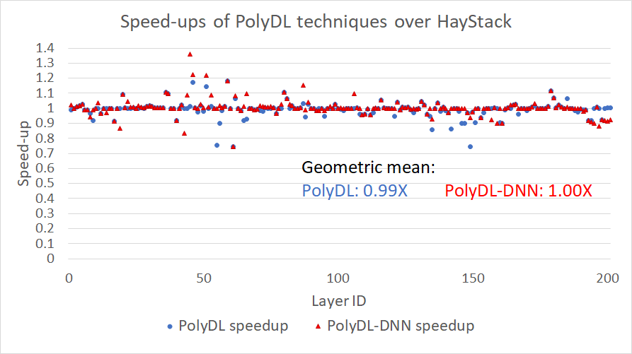
Figure 15 shows the speed-ups obtained by PolyDL and PolyDL-DNN with respect to Gysi et al.’s cache modeling work (Gysi et al. 2019). Their tool is termed HayStack and the same name is used in Figure 15. For most of the total 201 convolution layers (corresponding to the layers of fastrcnn, resnet, maskrcnn, xception, yolov2, mobilenet, alexnet, overfeat, googlenetv1, googlenetv3), the performances of code versions picked by PolyDL, and HayStack are identical. In some instances HayStack is better and in others PolyDL/PolyDL-DNN are higher performing.

On average, PolyDL-DNN achieves marginally better performance – it has a 1.002X speed-up over HayStack. Between PolyDL and HayStack, HayStack has a slight edge: PolyDL is at 0.99X performance levels of HayStack. We attribute the observed performance levels of the different methods to the nature of statistics we obtain using the PolyDL algorithms (working set sizes) and those that we obtain using the HayStack algorithm (the number of cache misses). It is straight-forward to relate the number of cache misses to the running time of the program using the cache latencies as done above. However, relating working set sizes to the running time of the program could be more complicated and the use of DNN techniques (i.e., PolyDL-DNN) is therefore superior to approximating the running time using cache latencies directly (i.e., PolyDL).

We observed that the running time of the HayStack tool is highly variable. In our experiments, HayStack took anywhere from a couple of seconds to 37 minutes to process a single code variant. On average, it takes $\sim$ 35 seconds. PolyDL’s running time was more uniform – it takes 2 - 3 seconds for any variant. Thus, PolyDL’s analysis is orders of magnitude faster than HayStack’s.

6.3.2. GEMMs

The GEMM operation is at the heart of deep learning (gem [n.d.]; Qin et al. 2020). The fully connected (FC) layers and multi-layer perceptrons map to GEMM operations: During the forward pass (for inference and for training too), the inputs and the weights are the two matrices that are multiplied. During the backward pass (for training), the error gradient with respect to the inputs and the weight matrices are multiplied.

Table 1. GEMM sizes

Workload	M	N	K	Workload	M	N	K
GNMT (Machine translation)	128	2048	4096	Synthetic	4096	4096	4096
GNMT (Machine translation)	320	3072	4096	Synthetic	1024	1024	32768
GNMT (Machine translation)	2048	4096	32	Synthetic	1024	32768	1024
DeepBench (General workload)	1024	16	500000	Synthetic	32768	1024	1024

We evaluate PolyDL’s efficacy on several matrix sizes. The GEMM operation is: $C=\beta.C+\alpha.A.B$ where C matrix’s dimensions are $M\times N$ while A and B matrices are of size $M\times K$ and $K\times N$ respectively. Table 1 lists the GEMM sizes evaluated. We use several problem sizes from DL workloads. We use four synthetic ones also to measure the performance obtained when all M, N, and K sizes are similar and when one of them is much higher than others (tall-skinny matrices, short-stout ones). We measure the performance of GEMMs when utilizing 32 processor cores.

Figure 16 shows the baseline GEMM code. We report the performance obtained by this code when compiled with the icc compiler and “-O3” flag in Figure 18 – designated as Baseline in the Figure. PolyDL framework generates several code variants for GEMM and ranks them. In Figure 17, we are showing one of the code variants generated. It is a two level tiled code. Tile sizes – M2_Tile, N2_Tile, K2_Tile, M1_Tile, N1_Tile, and K1_Tile are tunable parameters: PolyDL will vary these values and create distinct code variants. In the inner-most loops the GEMM microkernel is invoked for performing GEMM operation on matrix sizes M1_Tile, N1_Tile, and K1_Tile. Additionally, either loop it2 or jt2 could be made parallel. The PolyDL ranking algorithm will chose which loop is to be made parallel. The number of variants generated varies between 4 (for GEMM sizes M=1024,N=16,K=500000) and 1228 (for GEMM sizes M=4096,N=4096,K=4096). On average 491 code variants are explored for each set of GEMM sizes. We select the top 5% variants after PolyDL ranks them, and report the maximum performance obtained among those top 5% variants.

⬇

#pragma omp parallel for private(j, k)

for (i = 0; i < M; i++)

for (j = 0; j < N; j++)

for (k = 0; k < K; k++)

C[i][j] = beta * C[i][j] +

alpha * A[i][k] * B[k][j];

Figure 16. Baseline GEMM code

⬇

// First level of tiling

// Potential parallel loop1: it2

for (it2 = 0; it2 < M; it2 += M2_Tile) {

// Potential parallel loop2: jt2

for (jt2 = 0; jt2 < N; jt2 += N2_Tile) {

for (kt2 = 0; kt2 < K; kt2 += K2_Tile) {

// Second level of tiling

for(it1=it2;it1<it2+M2_Tile;it1+=M1_Tile){

for(jt1=jt2;jt1<jt2+N2_Tile;jt1+=N1_Tile){

for(kt1=kt2;kt1<kt2+K2_Tile;kt1+=K1_Tile){

//Call to GEMM microkernel of size:

//M1_Tile,N1_Tile,K1_Tile

microkernel(..)

}}}}}}

Figure 17. A code version generated for PolyDL

We compare the performance obtained by PolyDL with three other systems’: 1) Pluto (Bondhugula et al. 2008), a polyhedral source-to-source compiler, 2) AutoTVM, and 3) oneDNN. We input the code shown in Figure 16 to the Pluto tool and obtain tiled and parallelized code. We auto-tune for tile sizes: Pluto expects tile sizes to be inputted and we input several tile sizes. We report the maximum performance obtained by any of the tile size combinations in Pluto. To obtain the best performance possible from AutoTVM, we follow the GEMM optimization recipe provided on the TVM web pages (aut [n.d.]) and additionally explore many tile sizes and report the maximum performance obtained by any set of tile sizes.

Figure 18 depicts the performance obtained for various matrix sizes by different systems. In the graph, on the X-axis, the GEMM sizes (M, N, and K values as M_N_K) are shown. We observe that PolyDL-DNN and oneDNN performances are much higher than the other two, viz., Pluto and AutoTVM.

In 5 out of 8 GEMM sizes, PolyDL-DNN obtains substantially higher performance than oneDNN: For M=320 N=3072 K=4096 sizes, PolyDL-DNN is 2.6X higher performing than oneDNN. On average, PolyDL-DNN implementations are 1.24X faster compared to oneDNN’s (geometric average). PolyDL-DNN GEMM’s are 13.4X higher performing than baseline implementations. Pluto performance hovers around the same levels as that of the baseline code. On average, PolyDL-DNN achieves 11.0X speed-up over Pluto. We note that AutoTVM’s performance is orders of magnitude higher than baseline’s. This is partly explained by the fact that explicit vectorization encoded in the execution schedule (the most beneficial vectorization loop was already set manually) which resulted in good vectorization. PolyDL-DNN’s GEMMs were 2.7X faster compared to AutoTVM’s on average. The average (geo-mean) performance obtained in terms of GFLOPS/s across eight GEMM sizes by different systems, namely, Baseline, Pluto, AutoTVM, PolyDL-DNN, and oneDNN are 162, 197, 802, 2171, and 1745 respectively. We note that PolyDL achieves the highest performance among the cohort evaluated in this set of experiments.

In Figure 19, we show the performance spread among the different code variants that PolyDL system considered. The performances of all the code variants are normalized with respect to the maximum performance recorded for any variant. MIN denotes the lowest performance of any variant witnessed. Performances achieved by PolyDL-DNN (ranking of variants using the DNN model described in §4.2.2) and PolyDL (ranking of variants using the heuristics based on cache latencies as presented in §4.2.1) are shown. The closer the PolyDL’s and PolyDL-DNN’s performances are to 1.0 (the MAX line), the better it is – it shows that they are able to rank the variants correctly. We observe that performances of PolyDL-DNN picked code variants are closer to the maximum performance – within 0.95X of maximum performance. This shows that through compile-time modeling of data reuses in the loops as described in the paper, our techniques are able to identify high performance configurations for the loops.

We also show the performance obtained when the GEMM microkernels are used without any outer loop tuning in the graph – denoted as Microkernel. To measure the performance by using microkernels alone, we tile the baseline code shown in Figure 16 by factors of 16 in the three loop dimensions, and invoke the GEMM microkernel to perform matrix multiplications on matrices of sizes 16X16.

The microkernel-performance alone is quite low. Nevertheless, the use of microkernels alone speeds up baseline GEMM implementations by 2.2X. PolyDL-DNN achieves 6.0X speed-up over Microkernel implementations. This underscores the importance of performing outer loop optimizations to obtain high performance.

Between PolyDL and PolyDL-DNN, PolyDL-DNN picked code variants have higher performance, on average by a factor of 1.09X. For cost model based ranking of code variants, we use memory hierarchy’s latency and bandwidth values. While it fetches good rankings, DNN model is able to learn the latency and bandwidth values more accurately and can learn underlying hardware characteristics such as data prefetching automatically. Therefore, PolyDL-DNN’s rankings tend to be slightly better.

6.4. Evaluation of Operator Fusion

We evaluate the benefits of operator fusion algorithm presented in the paper ( §5) on two sequences: 1) batch normalization followed by the activation function ReLU, 2) convolution followed by the activation function ReLU6, which is a variant of ReLU. The activation function ReLU is defined as: $y=\max(x,0)$ , while ReLU6 is defined as $y=\min(\max(x,0),6)$ (Krizhevsky and Hinton 2010), that is, the output value is capped at 6. The batch normalization (bnorm for short) and ReLU sequence occurs frequently in CNN models including that of Resnet-50. We compare the performances of 1) bnorm, ReLU unfused code which forms the baseline 2) fused bnorm + ReLU operator using our fusion algorithm 3) fused bnorm + ReLU operator in the oneDNN library. There is no facility in AutoTVM to perform operator fusion automatically and therefore, we do not compare its performance on the sequence. Figure 21 shows the speed-ups obtained by our fused operator vis-a-vis the baseline code and oneDNN’s corresponding fused operator for the tensor sizes of all layers of CNN models we have considered in our experiments. The speed-ups achieved by the fused operator are 1.59X and 1.20X (geometric average across tensor sizes) compared to the unfused baseline code and the oneDNN’s operator respectively. Batch normalization is a memory bandwidth bound operation and therefore, fusing the subsequent ReLU operation reduces round trips to the main memory which substantially improves the performance.

We perform fusion experiments with the convolution and ReLU6 sequence too. We compare the performances of unfused and fused versions of the sequence. We note that ReLU6 is not supported in the oneDNN library. Researchers have found that ReLU6 improves the performance of image recognition models (Krizhevsky and Hinton 2010). However, ReLU6 is not widely adopted and it is not supported in the oneDNN library presumably because the high investment in supporting it is not justified. This underscores that 1) hand coding of a plethora of DNN primitives researchers experiment with is not scalable, 2) when an operator is not available in a library like oneDNN, it hampers the data scientists’ ability to quickly experiment and refine the DNN models. Therefore, automatic compilation techniques like the one developed in this paper are needed to address these bottlenecks.

Figure 21 shows the speed-ups of the fused operator when compared to the corresponding unfused operator. The ReLU6 activation function is applied on the output of the convolution. When the size of the output tensor is large, we observe a higher speed-up. When the output size is smaller, fusion has a marginal benefit. On average, the fused operator is 1.10X faster (geometric average). Furthermore, convolution is a compute-bound operation and therefore, the time spent in it is large relative to the time spent in the ReLU6 operation. This explains the contrasting speed-ups seen in the two sequences we have evaluated. For the bnorm + ReLU sequence, the speed-ups are larger because one, bnorm is a memory bound operation and two, the time spent in it is less compared to convolution. Consequently, the time spent in ReLU as a percentage of the time spent in bnorm is larger. Therefore, fusing the two operators shows larger performance gains for the bnorm + ReLU sequence.

7. Related Work

We discuss related works from polyhedral compilation, auto-tuning systems, deep learning DSL (Domain Specific Language) frameworks, and GEMM microkernel research.

Polyhedral compilation techniques have been developed for source-to-source code transformation for better cache locality and parallelization. The Pluto compiler (Bondhugula et al. 2008) derives an execution schedule for the code that attempts to minimize data reuse distances. The effect of the Pluto transformation will be that the iterations that use the same data will be executed close to each other in time and therefore, it will be cache friendly. The Pluto algorithm can accomplish fusion of loops too. However, Pluto’s performance can be far from what we can achieve with the use of microkernels that exploit the vector hardware effectively and by doing outer loop tuning in the way we have developed this work: In Section 6.3.2, we show that our techniques can produce on average 11.0X higher performing GEMM implementations. Furthermore, the Pluto algorithm experiences scalability issues – as the number of loops in a loop nest increases, the Pluto algorithm/tool can take exceedingly long time to derive a schedule. When we inputted the convolution followed by ReLU code sequence, the tool took several hours and did not produce an output. Kong et al. (Kong and Pouchet 2019) develop a framework to decompose a program into sub-parts and use customized criteria (as opposed to using a single objective function) – such as stride optimization, outer loop optimization, inner loop optimization to transform code. They show that their work without tiling transformation is able to achieve comparable results to that of Pluto.

The existing polyhedral compilation techniques fail to achieve performance competitive with hand tuned libraries. The main reason is, the loop transformations polyhedral techniques encode operate at a high level (source-to-source) and therefore, are unable to perform low-level orchestration of vector register allocation, detailed instruction scheduling (e.g., like that of the GEMM microkernel implementation described in §6.2). The latter aspects are crucial to achieving high performance on CPUs. An effective approach we believe is to use the polyhedral model based loop scheduling for outer loops for efficient use of cache hierarchy and to use microkernels for effective vectorization in the inner loops such as the one we have proposed in this paper.

Bondhugula et al. (Bondhugula et al. 2010) propose a fusion model that considers loss of parallelism with aggressive fusion. The number of available hardware prefetch streams is also used as a constraint to determine the beneficial fusion structures. In this paper, we have proposed a domain specific fusion algorithm that fuses heavy operators with element-wise operators. We have simplified the criteria for fusion while preserving parallelism. The patterns that our algorithm tackles occur frequently in DL workloads and our algorithm presents a first generic approach towards automatic fusions of operators in deep learning. Cornwall et al. (Cornwall et al. 2007) discuss using software engineering concepts like component based programming in the context of the development of a visual effects library. They use algorithmic skeletons to extract the iteration space for loops, and high level metadata for dependence analysis such that various optimizations can be applied. They propose using shifting as an enabler for fusion. Along with support for array-contraction which enables vectorization, the presented techniques result in good performance.

Compile-time modeling of cache behavior and in particular calculating the number of cache misses has been an active area of research (Ghosh et al. 1997; Bao et al. 2017; Gysi et al. 2019). Researchers have demonstrated good accuracy in predicting the number of cache misses on simulators. The modern computer architectures employ a hash based scheme to map memory addresses to cache sets (Yarom et al. 2015) which breaks the assumptions behind the cache miss analyses. In the present work, we model the behavior of caches as well. However, we do not model cache misses rather we consider data reuses and determine the size of cache needed to exploit the data reuses under conservative conditions. We ignore streaming accesses as their misses in cache will not be crucial in the resulting performance. Our analysis works on parallel code, whereas prior works are not equipped to handle parallel loops. Because of the these improvements, we show that we are able to accurately rank code variants in terms of performance. Our experimental evaluation comparing against the latest cache miss analysis work (Gysi et al. 2019) using sequential loop setting (§6.3.1) shows that the working set size approach we have adopted in our present work is as good as using cache misses for modeling of performance or is slightly better.

DSLs and Autotuning systems: Iterative compilation (Pouchet et al. 2008) and/or combined model-driven and iterative compilation techniques have been explored for program optimization (Pouchet et al. 2010). TVM (Chen et al. 2018a), a compiler for deep learning, introduces the concept of tensorization, where a unit of computation can be replaced with a microkernel written using hardware intrinsics. AutoTVM (Chen et al. 2018b) which is based on TVM, is targeted at accelerating deep learning workloads and uses machine learning to guide auto-tuning of deep learning primitives. We compared our techniques with AutoTVM in this paper and showed that the DL primitives created by PolyDL (our work) enjoy superior performance vis-a-vis AutoTVM. Further, the time it takes for our techniques to create high performance code is a fraction of the time AutoTVM takes. Tiramisu (Baghdadi et al. 2019) is a polyhedral model based compiler framework that introduces a scheduling language to allow the programmer to explore various program transformations. Halide (Ragan-Kelley et al. 2012) is a Domain Specific Language (DSL) and framework that introduces the distinction between an algorithm and its associated schedule. The DSL provides high level abstractions for the programmer to encode different schedules and thereby, explore different schedules in a productive way and discover high performance schedules. Adams et al (Adams et al. 2019) automate the task of finding optimal schedules in Halide using machine learning. In our present work, we take a compiler-centric approach: Using compiler-generated features we identify promising schedules (either through a heuristic based cost model or with the use of a neural network model). Because of these contrasting methodologies, Adams’ system would require a lot more training data (and therefore, resources to optimize a given code) than our PolyDL system. SWIRL (Venkat et al. 2019) is a system similar to Halide in the sense SWIRL also allows the programmer to specify the algorithm separately from its schedule. It allows one to encode numerous transformation recipes. Our PolyDL system can be complementary to SWIRL in that, the techniques developed in our work could be used to automate the task of deriving the beneficial transformation recipes automatically. TensorComprehensions (Vasilache et al. 2018) and Diesel (Elango et al. 2018) are two DSL systems developed for generating efficient code for GPUs. Both systems use the polyhedral model for code generation and provide auto-tuning capabilities. Unlike our system which is geared towards CPUs, both TensorComprehensions and Diesel target only GPUs. Since the considerations for optimizing code for GPUs are quite different from that for CPUs, their techniques are not directly applicable for CPUs.

GEMM microkernel optimizations: Goto and van de Geijn (Goto and Geijn 2008) focus on creating high-performance GEMMs by using a layered decomposition over the three micro-kernels, from which the others could be derived. The results show how these three lowest level decompositions can achieve high performance, thus resulting in an overall high performance for GEMM implementations. Springer et al. (Springer and Bientinesi 2018) use Tensor contraction for reducing the rank of matrices, followed by packing the tensor operands of the macro-kernel in the available caches, thus attaining the high performance. To remove the need of customization of microkernel for each hardware Veras et al. (Veras et al. 2016) present an automated approach by decomposing the microkernel (GEMM) into unit updates and building different algorithms over it. All these works focusing on microkernels are complementary to our approach: we could leverage microkernels created from any of these frameworks for our inner loops, thereby increasing the programmer productivity in our PolyDL approach.

Two level optimization of code: Barthou et al (Barthou et al. 2007) present a hierarchical compilation model, wherein the outer loops are optimized for data locality, while the inner loops are abstracted into kernels and are optimized for ILP (Instruction Level Parallelism) using the backend compiler. While at a high level, their approach and ours are similar, there are some crucial differences: 1) The outer loop optimization as developed in our work is more sophisticated (working set size enumeration and subsequent use of a DNN model for ranking of code variants) compared to the selection of tile sizes such that the data accessed in a tile fit in a certain level of cache as adopted in Barthou et al’s work. 2) The reliance on the backend compiler for kernel optimization in their work can lead to substantially lower performance compared to what is achievable through the use of microkernels. E.g., In our experimental evaluation (§6.3.2), we find that AutoTVM’s (their approach is nearly similar to AutoTVM’s) performance is substantially lower than PolyDL’s. 3) Their techniques are not applicable for parallel code and consequently, for multi-core architectures while handling of parallel code is baked into our techniques.

The BLIS framework (Zee et al. 2016) shows that BLAS routines can be instantiated using a single DGEMM microkernel. The microkernel needs to be customized for a given hardware and the programmer has to tune outer loops for cache use by choosing appropriate block (tile) sizes for the target architecture. Our PolyDL approach is similar to BLIS’s in spirit: we decompose the problem of optimizing an operator into two subproblems – one, performing outer loop optimization, and use of a microkernel for the inner loops. In our framework, we use novel polyhedral model based cache data reuse algorithms to perform outer loop optimizations automatically. Additionally, the use of a neural network based approach, and operator fusion algorithms are new and are beneficial for deep learning workloads.

8. Conclusion

In this paper, we presented novel compiler algorithms to derive high performing DL primitive implementations automatically and to perform operator fusions. We proposed a methodology to optionally use microkernels for the inner most loops of DL primitives to optimally use the vector pipelines of modern CPUs. With a combination of the above techniques, we demonstrated through experimental evaluation that we are able to match the performance of expert coded implementations of the Intel oneDNN library for CNNs and GEMMs. Additionally, because our method works at compile-time, we require much less time and compute resources to derive efficient implementations compared to auto-tuning systems such as AutoTVM. Our system – PolyDL will ease the development of computer architecture specific libraries by at most requiring the development of only a small number of microkernels. Additionally, it will allow data scientists to enjoy high performance on the new DNN architectures they develop immediately and automatically, without waiting for their DNN constructs to be implemented in a library by expert programmers.

References

(1)
goo ([n.d.]) [n.d.]. Google is AI first: 12 AI projects powering Google products. https://blog.aimultiple.com/ai-is-already-at-the-heart-of-google/
aut ([n.d.]) [n.d.]. How to optimize GEMM on CPU. https://tvm.apache.org/docs/tutorials/optimize/opt_gemm.html
lib ([n.d.]) [n.d.]. Library targeting Intel Architecture for specialized dense and sparse matrix operations, and deep learning primitives. https://github.com/hfp/libxsmm
int ([n.d.]) [n.d.]. oneAPI Deep Neural Network Library (oneDNN). https://github.com/oneapi-src/oneDNN
gem ([n.d.]) [n.d.]. Why GEMM is at the heart of deep learning. https://petewarden.com/2015/04/20/why-gemm-is-at-the-heart-of-deep-learning/
Adams et al. (2019) Andrew Adams, Karima Ma, Luke Anderson, Riyadh Baghdadi, Tzu-Mao Li, Michaël Gharbi, Benoit Steiner, Steven Johnson, Kayvon Fatahalian, Frédo Durand, et al. 2019. Learning to optimize halide with tree search and random programs. ACM Transactions on Graphics (TOG) 38, 4 (2019), 1–12.
Baghdadi et al. (2019) Riyadh Baghdadi, Jessica Ray, Malek Ben Romdhane, Emanuele Del Sozzo, Abdurrahman Akkas, Yunming Zhang, Patricia Suriana, Shoaib Kamil, and Saman Amarasinghe. 2019. Tiramisu: A polyhedral compiler for expressing fast and portable code. In Proceedings of the 2019 IEEE/ACM International Symposium on Code Generation and Optimization. IEEE Press, 193–205.
Bao et al. (2017) Wenlei Bao, Sriram Krishnamoorthy, Louis-Noel Pouchet, and P Sadayappan. 2017. Analytical modeling of cache behavior for affine programs. Proceedings of the ACM on Programming Languages 2, POPL (2017), 32.
Barthou et al. (2007) Denis Barthou, Sebastien Donadio, Patrick Carribault, Alexandre Duchateau, and William Jalby. 2007. Loop optimization using hierarchical compilation and kernel decomposition. In International Symposium on Code Generation and Optimization (CGO’07). IEEE, 170–184.
Baskaran et al. (2010) Muthu Manikandan Baskaran, Albert Hartono, Sanket Tavarageri, Thomas Henretty, Jagannathan Ramanujam, and Ponnuswamy Sadayappan. 2010. Parameterized tiling revisited. In Proceedings of the 8th annual IEEE/ACM international symposium on Code generation and optimization. ACM, 200–209.
Batra et al. (2018) Gaurav Batra, Zach Jacobson, Siddarth Madhav, Andrea Queirolo, and Nick Santhanam. 2018. Artificial-intelligence hardware: New opportunities for semiconductor companies. https://www.mckinsey.com/industries/semiconductors/our-insights
Bondhugula et al. (2010) Uday Bondhugula, Sanjeeb Dash, Oktay Gunluk, and Lakshminarayanan Renganarayanan. 2010. A model for fusion and code motion in an automatic parallelizing compiler. In 2010 19th International Conference on Parallel Architectures and Compilation Techniques (PACT). IEEE, 343–352.
Bondhugula et al. (2008) Uday Bondhugula, Albert Hartono, J. Ramanujam, and P. Sadayappan. 2008. A Practical Automatic Polyhedral Program Optimization System. In ACM SIGPLAN Conference on Programming Language Design and Implementation (PLDI).
Chen (2007) Chun Chen. 2007. Model-guided empirical optimization for memory hierarchy. University of Southern California.
Chen et al. (2018a) Tianqi Chen, Thierry Moreau, Ziheng Jiang, Lianmin Zheng, Eddie Yan, Haichen Shen, Meghan Cowan, Leyuan Wang, Yuwei Hu, Luis Ceze, et al. 2018a. $\{$ TVM $\}$ : An automated end-to-end optimizing compiler for deep learning. In 13th $\{$ USENIX $\}$ Symposium on Operating Systems Design and Implementation ( $\{$ OSDI $\}$ 18). 578–594.
Chen et al. (2018b) Tianqi Chen, Lianmin Zheng, Eddie Yan, Ziheng Jiang, Thierry Moreau, Luis Ceze, Carlos Guestrin, and Arvind Krishnamurthy. 2018b. Learning to optimize tensor programs. In Advances in Neural Information Processing Systems. 3389–3400.
Chung et al. (2004) I-Hsin Chung, Jeffrey K Hollingsworth, et al. 2004. Using information from prior runs to improve automated tuning systems. In Proceedings of the 2004 ACM/IEEE conference on Supercomputing. IEEE Computer Society, 30.
Cornwall et al. (2007) Jay LT Cornwall, Paul HJ Kelly, Phil Parsonage, and Bruno Nicoletti. 2007. Explicit dependence metadata in an active visual effects library. In International Workshop on Languages and Compilers for Parallel Computing. Springer, 172–186.
Darte et al. (2014) Alain Darte, Alexandre Isoard, et al. 2014. Parametric tiling with inter-tile data reuse. IMPACT 2014 (2014).
developers (2020) AutoTVM developers. 2020. AutoTVM’s X86 specific code. https://github.com/apache/incubator-tvm/blob/master/topi/python/topi/x86
Devlin et al. (2018) Jacob Devlin, Ming-Wei Chang, Kenton Lee, and Kristina Toutanova. 2018. Bert: Pre-training of deep bidirectional transformers for language understanding. arXiv preprint arXiv:1810.04805 (2018).
Elango et al. (2018) Venmugil Elango, Norm Rubin, Mahesh Ravishankar, Hariharan Sandanagobalane, and Vinod Grover. 2018. Diesel: DSL for linear algebra and neural net computations on GPUs. In Proceedings of the 2nd ACM SIGPLAN International Workshop on Machine Learning and Programming Languages. 42–51.
Feautrier (1996) Paul Feautrier. 1996. Automatic parallelization in the polytope model. In The Data Parallel Programming Model. Springer, 79–103.
Georganas et al. (2020) Evangelos Georganas, Kunal Banerjee, Dhiraj Kalamkar, Sasikanth Avancha, Anand Venkat, Michael Anderson, Greg Henry, Hans Pabst, and Alexander Heinecke. 2020. Harnessing Deep Learning via a Single Building Block. In 2020 IEEE International Parallel and Distributed Processing Symposium (IPDPS). IEEE, 222–233.
Ghosh et al. (1997) Somnath Ghosh, Margaret Martonosi, and Sharad Malik. 1997. Cache miss equations: An analytical representation of cache misses. In International Conference on Supercomputing. Citeseer, 317–324.
Girshick (2015) Ross Girshick. 2015. Fast R-CNN. arXiv:1504.08083 [cs.CV]
Goto and Geijn (2008) Kazushige Goto and Robert A van de Geijn. 2008. Anatomy of high-performance matrix multiplication. ACM Transactions on Mathematical Software (TOMS) 34, 3 (2008), 1–25.
Gysi et al. (2019) Tobias Gysi, Tobias Grosser, Laurin Brandner, and Torsten Hoefler. 2019. A fast analytical model of fully associative caches. In Proceedings of the 40th ACM SIGPLAN Conference on Programming Language Design and Implementation. ACM, 816–829.
Hartono et al. (2009) Albert Hartono, Muthu Manikandan Baskaran, Cédric Bastoul, Albert Cohen, Sriram Krishnamoorthy, Boyana Norris, Jagannathan Ramanujam, and Ponnuswamy Sadayappan. 2009. Parametric multi-level tiling of imperfectly nested loops. In Proceedings of the 23rd international conference on Supercomputing. ACM, 147–157.
He et al. (2017) Kaiming He, Georgia Gkioxari, Piotr Dollár, and Ross B. Girshick. 2017. Mask R-CNN. CoRR abs/1703.06870 (2017). arXiv:1703.06870 http://arxiv.org/abs/1703.06870
He et al. (2016) Kaiming He, Xiangyu Zhang, Shaoqing Ren, and Jian Sun. 2016. Deep residual learning for image recognition. In Proceedings of the IEEE conference on computer vision and pattern recognition. 770–778.
Heinecke et al. (2016) Alexander Heinecke, Greg Henry, Maxwell Hutchinson, and Hans Pabst. 2016. LIBXSMM: accelerating small matrix multiplications by runtime code generation. In SC’16: Proceedings of the International Conference for High Performance Computing, Networking, Storage and Analysis. IEEE, 981–991.
Hinton et al. (2012) Geoffrey Hinton, Li Deng, Dong Yu, George Dahl, Abdel-rahman Mohamed, Navdeep Jaitly, Andrew Senior, Vincent Vanhoucke, Patrick Nguyen, Brian Kingsbury, et al. 2012. Deep neural networks for acoustic modeling in speech recognition. IEEE Signal processing magazine 29 (2012).
Jouppi et al. (2017) Norman P Jouppi, Cliff Young, Nishant Patil, David Patterson, Gaurav Agrawal, Raminder Bajwa, Sarah Bates, Suresh Bhatia, Nan Boden, Al Borchers, et al. 2017. In-datacenter performance analysis of a tensor processing unit. In 2017 ACM/IEEE 44th Annual International Symposium on Computer Architecture (ISCA). IEEE, 1–12.
Kong and Pouchet (2019) Martin Kong and Louis-Noël Pouchet. 2019. Model-driven Transformations for Multi- and Many-core CPUs. In Proceedings of the 40th ACM SIGPLAN Conference on Programming Language Design and Implementation (Phoenix, AZ, USA) (PLDI 2019). https://doi.org/10.1145/3314221.3314653
Krizhevsky and Hinton (2010) Alex Krizhevsky and Geoff Hinton. 2010. Convolutional deep belief networks on cifar-10. Unpublished manuscript 40, 7 (2010), 1–9.
Krizhevsky et al. (2012) Alex Krizhevsky, Ilya Sutskever, and Geoffrey E Hinton. 2012. Imagenet classification with deep convolutional neural networks. In Advances in neural information processing systems. 1097–1105.
Pouchet et al. (2008) Louis-Noël Pouchet, Cédric Bastoul, Albert Cohen, and John Cavazos. 2008. Iterative optimization in the polyhedral model: Part II, multidimensional time. ACM SIGPLAN Notices 43, 6 (2008), 90–100.
Pouchet et al. (2010) Louis-Noël Pouchet, Uday Bondhugula, Cédric Bastoul, Albert Cohen, Jagannathan Ramanujam, and Ponnuswamy Sadayappan. 2010. Combined iterative and model-driven optimization in an automatic parallelization framework. In SC’10: Proceedings of the 2010 ACM/IEEE International Conference for High Performance Computing, Networking, Storage and Analysis. IEEE, 1–11.
Qin et al. (2020) Eric Qin, Ananda Samajdar, Hyoukjun Kwon, Vineet Nadella, Sudarshan Srinivasan, Dipankar Das, Bharat Kaul, and Tushar Krishna. 2020. Sigma: A sparse and irregular gemm accelerator with flexible interconnects for dnn training. In 2020 IEEE International Symposium on High Performance Computer Architecture (HPCA). IEEE, 58–70.
Ragan-Kelley et al. (2012) Jonathan Ragan-Kelley, Andrew Adams, Sylvain Paris, Marc Levoy, Saman Amarasinghe, and Frédo Durand. 2012. Decoupling algorithms from schedules for easy optimization of image processing pipelines. ACM Transactions on Graphics (TOG) 31, 4 (2012), 1–12.
Renganarayanan et al. (2007) Lakshminarayanan Renganarayanan, DaeGon Kim, Sanjay Rajopadhye, and Michelle Mills Strout. 2007. Parameterized tiled loops for free. In ACM SIGPLAN Notices, Vol. 42. ACM, 405–414.
Springer and Bientinesi (2018) Paul Springer and Paolo Bientinesi. 2018. Design of a high-performance gemm-like tensor–tensor multiplication. ACM Transactions on Mathematical Software (TOMS) 44, 3 (2018), 1–29.
Tavarageri et al. (2010) Sanket Tavarageri, Albert Hartono, Muthu Baskaran, Louis-Noël Pouchet, J Ramanujam, and P Sadayappan. 2010. Parametric tiling of affine loop nests. In Proc. 15th Workshop on Compilers for Parallel Computers. Vienna, Austria.
Tavarageri et al. (2013) Sanket Tavarageri, J Ramanujam, and P Sadayappan. 2013. Adaptive parallel tiled code generation and accelerated auto-tuning. The International Journal of High Performance Computing Applications 27, 4 (2013), 412–425.
Tiwari et al. (2009) Ananta Tiwari, Chun Chen, Jacqueline Chame, Mary Hall, and Jeffrey K Hollingsworth. 2009. A scalable auto-tuning framework for compiler optimization. In 2009 IEEE International Symposium on Parallel & Distributed Processing. IEEE, 1–12.
Vasilache et al. (2018) Nicolas Vasilache, Oleksandr Zinenko, Theodoros Theodoridis, Priya Goyal, Zachary DeVito, William S Moses, Sven Verdoolaege, Andrew Adams, and Albert Cohen. 2018. Tensor comprehensions: Framework-agnostic high-performance machine learning abstractions. arXiv preprint arXiv:1802.04730 (2018).
Venkat et al. (2019) Anand Venkat, Tharindu Rusira, Raj Barik, Mary Hall, and Leonard Truong. 2019. SWIRL: High-performance many-core CPU code generation for deep neural networks. The International Journal of High Performance Computing Applications 33, 6 (2019), 1275–1289.
Veras et al. (2016) Richard Michael Veras, Tze Meng Low, Tyler Michael Smith, Robert van de Geijn, and Franz Franchetti. 2016. Automating the last-mile for high performance dense linear algebra. arXiv preprint arXiv:1611.08035 (2016).
Verdoolaege (2010) Sven Verdoolaege. 2010. isl: An integer set library for the polyhedral model. In International Congress on Mathematical Software. Springer, 299–302.
Verdoolaege and Grosser (2012) Sven Verdoolaege and Tobias Grosser. 2012. Polyhedral Extraction Tool. In Second Int. Workshop on Polyhedral Compilation Techniques (IMPACT’12). Paris, France.
Wang and Yan (2020) Yao Wang and Eddie Yan. 2020. Auto-tuning a convolutional network for x86 CPU. https://docs.tvm.ai/tutorials/autotvm/tune_relay_x86.html
Wu et al. (2016) Yonghui Wu, Mike Schuster, Zhifeng Chen, Quoc V Le, Mohammad Norouzi, Wolfgang Macherey, Maxim Krikun, Yuan Cao, Qin Gao, Klaus Macherey, et al. 2016. Google’s neural machine translation system: Bridging the gap between human and machine translation. arXiv preprint arXiv:1609.08144 (2016).
Yarom et al. (2015) Yuval Yarom, Qian Ge, Fangfei Liu, Ruby B Lee, and Gernot Heiser. 2015. Mapping the Intel Last-Level Cache. IACR Cryptology ePrint Archive 2015 (2015), 905.
Zee et al. (2016) Field G Van Zee, Tyler M Smith, Bryan Marker, Tze Meng Low, Robert A Van De Geijn, Francisco D Igual, Mikhail Smelyanskiy, Xianyi Zhang, Michael Kistler, Vernon Austel, et al. 2016. The BLIS framework: Experiments in portability. ACM Transactions on Mathematical Software (TOMS) 42, 2 (2016), 1–19.