Variational Mutual Information Maximization Framework for VAE Latent Codes with Continuous and Discrete Priors

The very general form to define a mathematical model for inference for the real-world problem is the equation of the form

$$\mathbf{y}=\boldsymbol{\mathbf{W}}\mathbf{x},$$

(2.1)

where $\mathbf{y}$ is some variable that we want to infer with known value of variable $\mathbf{x}$ that is somehow related to $\mathbf{y}$, and $\boldsymbol{\mathbf{W}}$ defines some arbitrary transformation. As we mentioned in previous section, different phenomena in the real world are rarely deterministic and involve significant stochasticity. Thus, it is natural to fully model a particular real world phenomena in a from of probability distribution

$$p(\mathbf{x},\mathbf{y}).$$

(2.2)

Probability can be seen as the fuzzy form of logic that is applicable in cases with uncertainty. Logic is a set of rules for determining whether an argument true or false having set of prior arguments. The connection is that probability theory formalizes how to determine the likelihood of an argument given the likelihood of prior arguments.

Probabilistic models are used to describe systems with the use of probability distributions and random variables. Machine learning employs probabilistic models to recover true data generating distribution having set of samples $\mathcal{D}=\{\mathbf{x}^{(1)},\mathbf{x}^{(2)},\cdots,\mathbf{x}^{(m)}\}$ (where $m\geq 1$) drawn from true distribution $p_{data}(\mathbf{x})$. We wish to approximate the true distribution using a model $p_{\boldsymbol{\theta}}$ that represents some parametric family of distributions with parameters $\boldsymbol{\theta}$, such that $p_{\boldsymbol{\theta^{*}}}(\mathbf{x})\approx p_{data}(\mathbf{x})$. The most common approach to tackle this problem in modern machine learning and deep learning is Maximum Likelihood Estimation which results in optimal point estimate of $\boldsymbol{\theta}$ using estimator

$$\boldsymbol{\theta^{*}}=\mathop{\mathrm{arg\,max}}_{\boldsymbol{\theta}}p_{\boldsymbol{\theta}}(\mathcal{D}).$$

(2.3)

If the samples $\mathcal{D}$ from the true data distribution are i.i.d and using property of $\log$, equation 2.3 can be rewritten as

$$\boldsymbol{\theta^{*}}=\mathop{\mathrm{arg\,max}}_{\boldsymbol{\theta}}\sum_{i=1}^{m}[\log p_{\boldsymbol{\theta}}(\mathbf{x^{(i)}})]=\mathop{\mathrm{arg\,max}}_{\boldsymbol{\theta}}\mathbb{E}_{\mathbf{x}\sim\mathcal{D}}[\log p_{\boldsymbol{\theta}}(\mathbf{x})].$$

(2.4)

Actually, maximum likelihood estimation can be seen as minimizing KL divergence between empirical distribution $\hat{p}_{data}$ (represented by $\mathcal{D}$) of true data distribution $p_{data}(\mathbf{x})$ and the distribution represented by the model from chosen parametric family $p_{\boldsymbol{\theta}}$. KL divergence is a measure of how one probability distribution is different from another probability distribution. It has a perfect sense in our setting and then KL divergence can be defined as

$$D_{\mathit{KL}}(\hat{p}_{data}\;\|\;p_{\boldsymbol{\theta}})=\mathbb{E}_{\mathbf{x}\sim\hat{p}_{data}}[\log\hat{p}_{data}(\mathbf{x})-\log p_{\boldsymbol{\theta}}(\mathbf{x})].$$

(2.5)

Since the first term is constant, to minimize the KL divergence we need to minimize the negative second term which is the same as maximization setting in equation 2.4.

In the modern machine learning, this parametric distribution families are often represented by artificial neural networks (NN). I has been proven that this kind of models even with a single hidden layer with a finite number of units is capable of approximating any continuous function on compact subsets of real numbers [10]. Thus, the problem formulated in equation 2.4 can be seen as an optimization problem with respect to the parameters $\boldsymbol{\theta}$ which are the parameters of some NN. Optimization for NN when the are no closed form solution is usually done with gradient descent using gradients obtained by backpropagation algorithm [30].

In practice, for big datasets and models the optimization is done using stochastic gradient descent (SGD) by randomly drawing the minibatches of data $\mathcal{M}\subset\mathcal{D}$ and obtaining unbiased gradient estimator for likelihood maximization:

$\displaystyle\frac{1}{|\mathcal{D}|}\nabla_{\boldsymbol{\theta}}\textrm{ log }p_{\boldsymbol{\theta}}(\mathcal{D})=\mathbb{E}_{\mathcal{M}\sim\mathcal{D}}\bigg[\frac{1}{|\mathcal{M}|}\underset{\mathbf{x}\in\mathcal{M}}{\sum}\nabla_{\boldsymbol{\theta}}\textrm{ log }p_{\boldsymbol{\theta}}(\mathbf{x})\bigg].$

(2.6)

Discriminative models. A discriminative model is a model that defines conditional probability distribution $p(\mathbf{y}|\mathbf{x})$ for the target variable $\mathbf{y}$, given a known observation $\mathbf{x}$. When this kind models is applied to prediction tasks, we can formulate this as problem of unknown variable $\mathbf{y}$ estimation using observation $\mathbf{x}$. In this setting, maximum likelihood estimation can be extended to estimate parameters $\boldsymbol{\theta}$ of some distribution $p_{\boldsymbol{\theta}}(\mathbf{y}|\mathbf{x})$ that we want to use for an approximation of real conditional distribution $p_{true}(\mathbf{y}|\mathbf{x})$ to do inference or predictions. In that setting, given a dataset comprised of data points and respective predictions (labels) $\mathcal{D}=\{(\mathbf{x}^{(1)},\mathbf{y}^{(1)}),(\mathbf{x}^{(2)},\mathbf{y}^{(2)}),\cdots,(\mathbf{x}^{(m)},\mathbf{y}^{(m)})\}$ (where $m\geq 1$), the conditional maximum likelihood estimation has form

$$\boldsymbol{\theta^{*}}=\mathop{\mathrm{arg\,max}}_{\boldsymbol{\theta}}\sum_{i=1}^{m}[\log p_{\boldsymbol{\theta}}(\mathbf{y^{(i)}}|\mathbf{x^{(i)}})]=\mathop{\mathrm{arg\,max}}_{\boldsymbol{\theta}}\mathbb{E}_{(\mathbf{x},\mathbf{y})\sim\mathcal{D}}[\log p_{\boldsymbol{\theta}}(\mathbf{y}|\mathbf{x})].$$

(2.7)

Generative models. This kind of models aims to find all factors that explain target phenomena or data and define distribution $p(\mathbf{x},\mathbf{y})$. From the previous section viewpoint, we can see it as a probabilistic model that simultaneously models distribution of observations and predictions. This allows one to obtain discriminative distribution $p(\mathbf{y}|\mathbf{x})$ as well as generative one $p(\mathbf{x}|\mathbf{y})$ and individual distributions of $p(\mathbf{x})$ and $p(\mathbf{y})$ by marginalization and Bayes rule.

Machine learning and Deep Learning approaches face probability distributions over a various number of random variables. These distributions may involve direct interactions between relatively few variables in comparison to their total number. Using a single function to describe the entire joint probability distribution over all random variables may be inefficient and does not provide a way to incorporate knowledge about direct dependencies between this variables into a model.

Directed graphical models or Bayesian networks is a family of probability distributions that provide compact parametrization that can be naturally described using a directed graph. Bayesian networks represent probability distributions that can be formed via products of smaller conditional probability distributions (one for each variable). By having probability of this form, we are introducing assumptions that certain variables are independent and others are dependent into our model. The parametrization idea is next, having joint probability of all present random variables, we can decompose it using chain rule as

$$p(\mathbf{x}_{1},\mathbf{x}_{2},\ldots,\mathbf{x}_{n})=p(\mathbf{x}_{1})p(\mathbf{x}_{2}|\mathbf{x}_{1})\cdots p(\mathbf{x}_{n}|\mathbf{x}_{n-1},\ldots,\mathbf{x}_{2},\mathbf{x}_{1})$$

(2.8)

In a Bayesian network model representation, the components of factorized right-hand side of the Eq.2.8 is simplified when prior assumption about independence of certain variables are incorporated into the model. Then, each factor for $\mathbf{x}_{i}$ depends only on a particular set of ancestor variables $\mathbf{x}_{A_{i}}$ resulting in

$$p(\mathbf{x}_{i}|\mathbf{x}_{i-1},\ldots,\mathbf{x}_{1})=p(\mathbf{x}_{i}|\mathbf{x}_{A_{i}}).$$

(2.9)

In this setting, we can reformulate the initial joint distribution as

$$p(\mathbf{x}_{1},\mathbf{x}_{2},\ldots,\mathbf{x}_{n})=\prod_{i=1}^{n}p(\mathbf{x}_{i}|\mathbf{x}_{A_{i}})$$

(2.10)

Distributions and models of this form can be naturally expressed as directed acyclic graphs (DAG), where nodes represent random variables $\mathbf{x}_{i}$ and edges represent their relationships. For instance, consider a probabilistic directed model over random variables $\mathbf{a},\mathbf{b},\mathbf{c},\mathbf{d},\mathbf{e}$ which is represented by figure 2.1. This graphical model enables one directly incorporate relationships between random variables into probabilistic model of the distribution. As you can see, $\mathbf{a}$ and $\mathbf{c}$ (as well as $\mathbf{a}$ and $\mathbf{b}$) interact directly, but $\mathbf{a}$ and $\mathbf{e}$ interact only indirectly through $\mathbf{c}$ forming markov chain.

Such model can be represented by joint probability distribution that is factorized as

$$p(\mathbf{a},\mathbf{b},\mathbf{c},\mathbf{d},\mathbf{e})=p(\mathbf{a})p(\mathbf{b}|\mathbf{a})p(\mathbf{d}|\mathbf{b})p(\mathbf{e}|\mathbf{c})p(\mathbf{c}|\mathbf{a},\mathbf{b})$$

(2.11)

Formal definition. Directed probabilistic model is a directed graph $\mathbf{G}$=($\mathbf{V}$,$\mathbf{E}$) where each random variable $\mathbf{x}_{i}$ corresponds to node i $\in$ $\mathbf{V}$ and $\mathbf{E}$ represents relationships between this variables. One conditional probability distribution per node $p(\mathbf{x}_{i}|\mathbf{x}_{A_{i}})$ from factorized joint distribution over all variables. It specifies probability distribution of $\mathbf{x}_{i}$ with respect to its ancestors given values $\mathbf{x}_{A_{i}}$. The advantage of structured probabilistic modelling is that it reduces the modelling cost of probability distributions to explain some particular phenomena. Also, it makes it is easier to perform learning and inference. The main advantage is possibility to avoid modeling particular dependencies with use of prior assumptions. These models represent dependencies as edges. Leaving any particular edge out, the model incorporates an assumption that some random variables do not require direct interaction.

Independence assumptions made when modelling Bayesian network are important since they define key properties of the particular model. They represent prior understanding of the phenomena that we are trying to model and this information may provide useful insights for performing inference. There are three key dependence structures for modeling probabilistic models with three random variables (nodes). Let Bayes net represent three random variables $\mathbf{A}$, $\mathbf{B}$, and $\mathbf{C}$. Then these three dependence structures (illustrated in figure 2.2) can be formulated as follows

• •

  Cascade. In that case directed graphical model represent dependencies as $\mathbf{A}$ $\rightarrow$ $\mathbf{B}$ $\rightarrow$ $\mathbf{C}$. Thus, if variable $\mathbf{B}$ is observed then $\mathbf{A}$ and $\mathbf{C}$ are conditionally independent. This is so since in that setting, the variable B contains everything that define outcome $\mathbf{C}$.

• •

  Common parent. When Bayesian model has form of $\mathbf{A}$ $\leftarrow$ $\mathbf{B}$ $\rightarrow$ $\mathbf{C}$ and $\mathbf{B}$ is observed then $\mathbf{A}$ and $\mathbf{C}$ are conditionally independent again. In that case, this is so since $\mathbf{B}$ completely defines outcome $\mathbf{A}$ and $\mathbf{B}$ independently.

• •

  V-structure. In that case the model has form of $\mathbf{A}$ $\rightarrow$ $\mathbf{C}$ $\leftarrow$ $\mathbf{B}$. It means that knowledge of outcome $\mathbf{C}$ couples $\mathbf{A}$ and $\mathbf{B}$. Otherwise, $\mathbf{A}$ and $\mathbf{B}$ are independent.

Latent variable models (LVM) is powerful approach to probabilistic modelling that deals with a set of observed variables with latent, or hidden, variables. This modelling approach is extremely useful in cases when some data might be naturally unobserved. When a joint distribution over observable and latent variables is defined, the distribution of the observations can be obtained by marginalization of the latent variable. This approach makes it possible to model complex data distributions and express them in terms of more tractable joint distributions. The common example of a latent variable model is the Gaussian mixture distribution where the latent variable is mixture component label. The structure of such probabilistic models can be represented in a graphical manner. For instance, as a directed acyclic graph (DAG), or Bayesian network.

In general, latent variable model is a model that defines joint probability distribution over two random variables $\mathbf{x}$ and $\mathbf{z}$

$$p(\mathbf{x},\mathbf{z}),$$

(2.12)

where $\mathbf{x}$ are observable variable (represented by data points during training) and $\mathbf{z}$ that are unobserved. Latent variables may appear naturally, from the structure of the problem, because something wasn’t measured, because of faulty sensors, occlusion, privacy. These models can be represented as directed or undirected. There exist both discriminative and generative LVM and those which combine them as Variational Autoencoder [22, 29]. The goal of LVM is to express distribution $p(\mathbf{x})$ of the observable variables using smaller number of latent variables [19]. It is done by first decomposing the joint distribution $p(\mathbf{x},\mathbf{z})$ into posterior distribution $p(\mathbf{x}|\mathbf{z})$ and prior $p(\mathbf{z})$ resulting in

$$p(\mathbf{x},\mathbf{z})=p(\mathbf{x}|\mathbf{z})p(\mathbf{z}).$$

(2.13)

Then, the distribution $p(\mathbf{x})$ is obtained by marginalization of latent variable

$$p(\mathbf{x})=\int p(\mathbf{x}|\mathbf{z})p(\mathbf{z})d\mathbf{z}$$

(2.14)

to which can be appllied such estimation techniques as maximum likelihood estimation (eq. 2.4). The integration procedure in general can be intractable, as in case of deep neural networks, except cases when the distributions $p(\mathbf{x}|\mathbf{z})$ and $p(\mathbf{z})$ have specific form and closed form solution is achievable.

Gaussian mixture models (GMMs) is a kind of widely used latent variable models in machine learning. In this setting, each data point is a tuple $(\mathbf{x}_{i},\mathbf{z}_{i})$ where $\mathbf{x}_{i}$$\in$$\mathbb{R}^{d}$ and $\mathbf{z}_{i}$ is a discrete random variable of K categories. The joint distribution $p(\mathbf{x},\mathbf{z})=p(\mathbf{x}|\mathbf{z})p(\mathbf{z})$ is a directed model (see fig 2.3), where $p(\mathbf{z}=k)=\pi_{k}$ for some vector of class probabilities $\pi\in\Delta_{K-1}$ and then

$$p(\mathbf{x}|\mathbf{z}=k)=\mathcal{N}(\mathbf{x};\mu_{k},\Sigma_{k})$$

(2.15)

which is multivariate Gaussian distribution parametrized by $\mu_{k}$ and $\Sigma_{k}$. GMM model defines observed data as points that come from K Gaussian clusters with proportions represented by $\pi_{1},\ldots,\pi_{K}$. The resulting observed data point probability has form of

$$p(\mathbf{x})=\sum_{n=1}^{K}p(\mathbf{x}|\mathbf{z}=n)p(\mathbf{z}=n)=\sum_{n=1}^{K}\pi_{n}\mathcal{N}(\mathbf{x};\mu_{n},\Sigma_{n})$$

(2.16)

If we wish to sample new data point from that distribution, first we sample a category k and then sample a point from Gaussian distribution with respective parameters $\mu_{k}$ and $\Sigma_{k}$.

Expectation Maximization (EM) algorithm is widely used algorithm for fitting directed LVM models which aim is the same as in the case of maximum likelihood estimation - maximize data likelihood (see section 2.4.1) $p_{\boldsymbol{\theta}}(\mathbf{x})$ for some model $p_{\boldsymbol{\theta}}(\mathbf{x},\mathbf{z})$ of particular parametric family with parameters $\boldsymbol{\theta}$. Having collected observable data points $\mathcal{D}=\{\mathbf{x}^{(1)},\mathbf{x}^{(2)},\cdots,\mathbf{x}^{(m)}\}$ (where $m\geq 1$), we wish to maximize marginal log-likelihood of the data

$$\log[p_{\boldsymbol{\theta}}(\mathcal{D})]=\mathbb{E}_{\mathbf{x}\sim\mathcal{D}}[\log p_{\boldsymbol{\theta}}(\mathbf{x})]=\mathbb{E}_{\mathbf{x}\sim\mathcal{D}}[\mathbb{E}_{\mathbf{z}\sim p_{\boldsymbol{\theta}}(\mathbf{z}|\mathbf{x})}[\log p_{\boldsymbol{\theta}}(\mathbf{x},\mathbf{z})]].$$

(2.17)

This optimization objective is more complex than log-likelihood maximization in maximum likelihood estimation setting, even for directed graphical models. It is not possible to derive a closed form solution for the parameters even when the distributions represent some conventional distribution families.

On the other hand, we can employ iterative EM algorithm that may converge to optimal solution. This algorithm relies on assumption that it is possible to obtain posterior distribution $p_{\boldsymbol{\theta}}(\mathbf{z}|\mathbf{x})$. There are cases when it is not possible and there arise variational inference methods that will be covered later. The EM algorithm relies on two steps, first we start with some arbitrary parameters $\boldsymbol{\theta}_{0}$ and then repeat the following steps until convergence with t=0,1,2…

• •

  E-step. For each $\mathbf{x}$ $\in$ $\mathcal{D}$, compute posterior $p_{\boldsymbol{\theta_{t}}}(\mathbf{z}|\mathbf{x})$.

• •

  M-step. Obtain new weights by

  $$\boldsymbol{\theta_{t+1}}=\mathop{\mathrm{arg\,max}}_{\boldsymbol{\theta}}\mathbb{E}_{\mathbf{x}\sim\mathcal{D}}[\mathbb{E}_{\mathbf{z}\sim p_{\boldsymbol{\theta}_{t}}(\mathbf{z}|\mathbf{x})}[\log p_{\boldsymbol{\theta}_{t}}(\mathbf{x},\mathbf{z})]]=\mathop{\mathrm{arg\,max}}_{\boldsymbol{\theta}}\mathbb{E}_{\mathbf{x}\sim\mathcal{D}}[\log p_{\boldsymbol{\theta}_{t}}(\mathbf{x})].$$

  (2.18)

Since the optimization procedure is non-convex, EM is not guaranteed to reach global optimum solution. However, EM in practical application converges to a feasible local optimum solution. The performance of EM algorithm depends on the initial choice of parameters $\boldsymbol{\theta}_{0}$. Different initialization may lead to different local optima. Techniques for selecting parameters for particular probabilistic model to which EM is applicable is an active separate direction in machine learning research.

Inference as optimization In this setting, consider LVM again with observed variables $\mathbf{x}$ and latent variables $\mathbf{z}$. For fitting the particular model we wish to obtain $\log p_{\boldsymbol{\theta}}(\mathbf{x})$ for the observed data. There are cases when it is costly and intractable to marginalize the latent variable $\mathbf{z}$. Instead, it is convenient to maximize variational lower bound or evidence lower bound (ELBO). The other used term for this objective is variational free energy proposed by Richard Feynman in 1972. Evidence lower bound can be defined as

$$\mathcal{L}(\mathbf{z},\boldsymbol{\theta},q)=\log p_{\boldsymbol{\theta}}(\mathbf{x})-D_{\mathit{KL}}(q(\mathbf{z})\;\|\;p_{\boldsymbol{\theta}}(\mathbf{z}|\mathbf{x}))$$

(2.19)

where q is an arbitrary distribution. We can derive it as follows

	$\displaystyle\textrm{log }p_{\boldsymbol{\theta}}(\mathbf{x})$	$\displaystyle=\mathbb{E}_{q(\mathbf{z})}\Big[\textrm{log }p_{\boldsymbol{\theta}}(\mathbf{x})\Big]$		(2.20)
		$\displaystyle=\mathbb{E}_{q(\mathbf{z})}\bigg[\textrm{log}\left\{\frac{p_{\boldsymbol{\theta}}(\mathbf{x},\mathbf{z})}{q(\mathbf{z})}\frac{q(\mathbf{z})}{p_{\boldsymbol{\theta}}(\mathbf{z}|\mathbf{x})}\right\}\bigg]$		(2.21)
		$\displaystyle=\mathbb{E}_{q(\mathbf{z})}\bigg[\textrm{log}\left\{\frac{p_{\boldsymbol{\theta}}(\mathbf{x},\mathbf{z})}{q(\mathbf{z})}\right\}\bigg]+\mathbb{E}_{q(\mathbf{z})}\bigg[\textrm{log}\left\{\frac{q(\mathbf{z})}{p_{\boldsymbol{\theta}}(\mathbf{z}|\mathbf{x})}\right\}\bigg]$		(2.22)
		$\displaystyle=\mathcal{L}(\mathbf{z},\boldsymbol{\theta},q)+D_{\mathit{KL}}(q(\mathbf{z})\;\|\;p_{\boldsymbol{\theta}}(\mathbf{z}|\mathbf{x})).$		(2.23)

Since the KL divergence term is non-negative, ELBO can be seen as lower bound on true data log likelihood, meaning

$$\log p_{\boldsymbol{\theta}}(\mathbf{x})\geq\mathcal{L}(\mathbf{z},\boldsymbol{\theta},q).$$

(2.24)

We can interpret it as an approximation to the true data likelihood and it is tight when

$$D_{\mathit{KL}}(q(\mathbf{z})\;\|\;p_{\boldsymbol{\theta}}(\mathbf{z}|\mathbf{x}))=0\iff q(\mathbf{z})=p_{\boldsymbol{\theta}}(\mathbf{z}|\mathbf{x}),$$

(2.25)

and then

$$\log p_{\boldsymbol{\theta}}(\mathbf{x})=\mathcal{L}(\mathbf{z},\boldsymbol{\theta},q).$$

(2.26)

With respect to aforementioned theoretic insights, it is valid to interpret inference as the procedure optimizing $\mathcal{L}(\mathbf{z},\boldsymbol{\theta},q)$ with respect to q. Exact inference can match $\mathcal{L}(\mathbf{z},\boldsymbol{\theta},q)$ to $\log p_{\boldsymbol{\theta}}(\mathbf{x})$ if q represents a set of distributions that includes $p_{\boldsymbol{\theta}}(\mathbf{z}|\mathbf{x})$. Moreover, in some cases when this distributions have particular form, this optimization can be done in a closed form.

Variational lower bound. Function $g(\xi,\mathbf{y})$ is called variational lower bound for $f(\mathbf{y})$ iff for all $\xi$ and for all $\mathbf{y}$ it follows $f(\mathbf{y})$ $\geq$ $g(\xi,\mathbf{y})$ and for any $\mathbf{y}_{0}$ there exists $\xi(\mathbf{y}_{0})$ such that $f(\mathbf{y}_{0})$ = $g(\xi(\mathbf{y}_{0}),\mathbf{y}_{0})$. If it is possible to find such variational lower bound then, instead of solving

$$\mathbf{y}^{*}=\mathop{\mathrm{arg\,max}}_{\mathbf{y}}f(\mathbf{y}),$$

(2.27)

it is possible to perform block-coordinate updates of $g(\xi(\mathbf{y}),\mathbf{y})$, meaning

$$\mathbf{y}_{t}=\mathop{\mathrm{arg\,max}}_{\mathbf{y}}g(\xi_{t-1},\mathbf{y})\ ,\ \xi_{t}=\xi(\mathbf{y}_{t})=\mathop{\mathrm{arg\,max}}_{\xi}g(\xi,\mathbf{y}_{t})$$

(2.28)

In the setting of latent variable models, we wish to maximize marginal data log-likelihood $\log p_{\boldsymbol{\theta}}(\mathbf{x})$. In the Section 2.4.3, we described a common method for fitting this kind of models - expectation maximization algorithm. This algorithm can be also described from the perspective of maximization of variational lower bound on marginal data log-likelihood (ELBO). From (2.23) we know that

$$\log p_{\boldsymbol{\theta}}(\mathbf{x})=\mathcal{L}(\mathbf{z},\boldsymbol{\theta},q)+D_{\mathit{KL}}(q(\mathbf{z})\;\|\;p_{\boldsymbol{\theta}}(\mathbf{z}|\mathbf{x}))\ and\ \log p_{\boldsymbol{\theta}}(\mathbf{x})\geq\mathcal{L}(\mathbf{z},\boldsymbol{\theta},q).$$

(2.29)

Then, to maximize $\log p_{\boldsymbol{\theta}}(\mathbf{x})$ we can maximize ELBO when it is tight. Thus, we can reformulate EM algorithm as follows: starting with $\boldsymbol{\theta}_{0}$ and then repeating the following steps until convergence with t=0,1,2…

• •

  E-step. For each $\mathbf{x}$ $\in$ $\mathcal{D}$ compute posterior which is equivalent to making ELBO tight by finding q that maximizes it:

  $$q(\mathbf{z})=\mathop{\mathrm{arg\,max}}_{q}\mathcal{L}(\mathbf{z},\boldsymbol{\theta},q)=\mathop{\mathrm{arg\,min}}_{q}D_{\mathit{KL}}(q(\mathbf{z})\;\|\;p_{\boldsymbol{\theta}_{t}}(\mathbf{z}|\mathbf{x}))=p_{\boldsymbol{\theta}_{t}}(\mathbf{z}|\mathbf{x})$$

  (2.30)

• •

  M-step. Having ELBO tight to true data log-likelihood, we can find the parameters $\boldsymbol{\theta_{t+1}}$ that maximize it

  $$\boldsymbol{\theta_{t+1}}=\mathop{\mathrm{arg\,max}}_{\boldsymbol{\theta}}\mathcal{L}(\mathbf{z},\boldsymbol{\theta},q)=\mathop{\mathrm{arg\,max}}_{\boldsymbol{\theta}}\log p_{\boldsymbol{\theta}_{t}}(\mathbf{x})=\mathop{\mathrm{arg\,max}}_{\boldsymbol{\theta}}\mathbb{E}_{\mathbf{z}}[\log p_{\boldsymbol{\theta}_{t}}(\mathbf{x},\mathbf{z})].$$

  (2.31)

This process monotonically increases the lower bound and converges to stationary point of $\log p_{\boldsymbol{\theta}^{*}}(\mathbf{x})$. If the true posterior $p_{\boldsymbol{\theta}}(\mathbf{z}|\mathbf{x})$ is intractable to compute, then we may do search for the closest $q(\mathbf{z})$ among tractable distributions by solving optimization problem or represent this distribution by the neural network as in [22, 29]. In that case, $q(\mathbf{z})$ becomes variational approximation to $p_{\boldsymbol{\theta}}(\mathbf{z}|\mathbf{x})$.

We wish to be able to perform efficient approximate inference and learning in probabilistic directed latent variable models with continuous latent variables and/or parameters that have intractable posterior distributions and big datasets. In this case, the conventional EM algorithm will not work since the E step requires the posterior distribution to be known and tractable. If it is not, then marginal likelihood is also intractable. The mean-field Variational Bayes approach requires closed form solutions to the approximate posterior $p_{\boldsymbol{\theta}}(\mathbf{z}|\mathbf{x})$, which can be intractable in general case when dealing with large datasets and complicated likelihood $p_{\boldsymbol{\theta}}(\mathbf{x}|\mathbf{z})$ that can be represented by neural networks. Basically, we need to obtain this distribution to perform E step

$\displaystyle q(\mathbf{z})=\prod_{i=1}^{n}q(\mathbf{z}_{i})=\prod_{i=1}^{n}p_{\boldsymbol{\theta}}(\mathbf{z}_{i}|\mathbf{x}_{i})=\prod_{i=1}^{n}\frac{p_{\boldsymbol{\theta}}(\mathbf{z}_{i}|\mathbf{x}_{i})p_{\boldsymbol{\theta}}(\mathbf{z}_{i})}{\int p_{\boldsymbol{\theta}}(\mathbf{z}_{i}|\mathbf{x}_{i})p_{\boldsymbol{\theta}}(\mathbf{z})dz}.$

(3.1)

However, in general setting the denominator is intractable.

In [22, 29] the authors proposed solution to the problems of the aforementioned scenario. Lets consider such setting of probabilistic latent variable models when we have dataset $\mathbf{X}$= $\{\mathbf{x}^{(i)}\}_{i=1}^{N}$ of N i.i.d. data samples of some observed random variable $\mathbf{x}$. Under assumption that the observed data came from some generative random process, involving latent random variable $\mathbf{z}$, the process is defined as follows: $\mathbf{z}$ comes from prior distribution $p_{\boldsymbol{\theta}^{*}}(\mathbf{z})$ and the observed sample $\mathbf{x}$ is generated by some process defined by $p_{\boldsymbol{\theta}^{*}}(\mathbf{x}|\mathbf{z})$. We assume that this two distributions that define generative process come from parametric families $p_{\boldsymbol{\theta}}(\mathbf{x}|\mathbf{z})$ and $p_{\boldsymbol{\theta}}(\mathbf{z})$ that are differentiable almost everywhere. In this setting, true parameters $\boldsymbol{\theta}^{*}$ and $\mathbf{z}$ are unknown.

The [22, 29] authors propose a scalable solution for learning LVM that addresses intractability of posterior distributions and big datasets. They propose approximate ML or MAP estimation for the parameters $\boldsymbol{\theta}$ that allow one to analyze some hidden process as well as generate new data samples by mimicking the true generative process defined by $p_{\boldsymbol{\theta}^{*}}(\mathbf{x}|\mathbf{z})$ and $p_{\boldsymbol{\theta}^{*}}(\mathbf{z})$. Also, they provide method for efficient approximate posterior inference of $\mathbf{z}$ given $\mathbf{x}$.

The core idea behind the proposed approach is to represent intractable posterior distribution $p_{\boldsymbol{\theta}}(\mathbf{z}|\mathbf{x})$ by a flexible variational approximation $q_{\boldsymbol{\phi}}(\mathbf{z}|\mathbf{x})$ (a neural network). Thus, authors define recognition model as a probabilistic encoder $q_{\boldsymbol{\phi}}(\mathbf{z}|\mathbf{x})$ and $p_{\boldsymbol{\theta}}(\mathbf{x}|\mathbf{z})$ as probabilistic decoder, both represented by neural networks with parameters $\boldsymbol{\phi}$ and $\boldsymbol{\theta}$ respectively. The resulting directed probabilistic model is depicted in Figure 3.1.

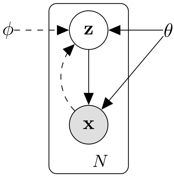
In this setting, we again wish to maximize marginal data log-likelihood $\textrm{log }p_{\boldsymbol{\theta}}(\mathbf{x})$ by maximizing its variational lower bound. We can derive variational lower bound (ELBO) on true data log-likelihood in the current setting as follows

	$\displaystyle\textrm{log }p_{\boldsymbol{\theta}}(\mathbf{x})$	$\displaystyle=\mathbb{E}_{q_{\boldsymbol{\phi}}(\mathbf{z}|\mathbf{x})}\Big[\textrm{log }p_{\boldsymbol{\theta}}(\mathbf{x})\Big]$		(3.2)
		$\displaystyle=\mathbb{E}_{q_{\boldsymbol{\phi}}(\mathbf{z}|\mathbf{x})}\bigg[\textrm{log}\left\{\frac{p_{\boldsymbol{\theta}}(\mathbf{x},\mathbf{z})}{q_{\boldsymbol{\phi}}(\mathbf{z}|\mathbf{x})}\frac{q_{\boldsymbol{\phi}}(\mathbf{z}|\mathbf{x})}{p_{\boldsymbol{\theta}}(\mathbf{z}|\mathbf{x})}\right\}\bigg]$
		$\displaystyle=\mathbb{E}_{q_{\boldsymbol{\phi}}(\mathbf{z}|\mathbf{x})}\bigg[\textrm{log}\left\{\frac{p_{\boldsymbol{\theta}}(\mathbf{x},\mathbf{z})}{q_{\boldsymbol{\phi}}(\mathbf{z}|\mathbf{x})}\right\}\bigg]+\mathbb{E}_{q_{\boldsymbol{\phi}}(\mathbf{z}|\mathbf{x})}\bigg[\textrm{log}\left\{\frac{q_{\boldsymbol{\phi}}(\mathbf{z}|\mathbf{x})}{p_{\boldsymbol{\theta}}(\mathbf{z}|\mathbf{x})}\right\}\bigg]$
		$\displaystyle=\mathcal{L}(\boldsymbol{\theta},\boldsymbol{\phi})+D_{\mathit{KL}}(q_{\boldsymbol{\phi}}(\mathbf{z}|\mathbf{x})\;\|\;p_{\boldsymbol{\theta}}(\mathbf{z}|\mathbf{x})).$

Then, the variational lower bound can be decomposed as

$$\mathcal{L}(\boldsymbol{\theta},\boldsymbol{\phi})=\mathbb{E}_{q_{\boldsymbol{\phi}}(\mathbf{z}|\mathbf{x})}\bigg[\textrm{log}\left\{\frac{p_{\boldsymbol{\theta}}(\mathbf{x}|\mathbf{z})p_{\boldsymbol{\theta}}(\mathbf{x})}{q_{\boldsymbol{\phi}}(\mathbf{z}|\mathbf{x})}\right\}\bigg]=\mathbb{E}_{q_{\boldsymbol{\phi}}(\mathbf{z}|\mathbf{x})}[\log p_{\boldsymbol{\theta}}(\mathbf{x}|\mathbf{z})]-D_{\mathit{KL}}(q_{\boldsymbol{\phi}}(\mathbf{z}|\mathbf{x})\;\|\;p_{\boldsymbol{\theta}}(\mathbf{z})),$$

(3.3)

which we wish to maximize with respect to parameters $\boldsymbol{\theta}$ and $\boldsymbol{\phi}$ to maximize the true marginal data log-likelihood. Thus, the final objective has form of

$$\boldsymbol{\theta^{*}},\ \boldsymbol{\phi}^{*}=\mathop{\mathrm{arg\,max}}_{\boldsymbol{\theta},\boldsymbol{\phi}}\mathcal{L}(\boldsymbol{\theta},\boldsymbol{\phi})=\mathop{\mathrm{arg\,max}}_{\boldsymbol{\theta},\boldsymbol{\phi}}\ \mathbb{E}_{q_{\boldsymbol{\phi}}(\mathbf{z}|\mathbf{x})}[\log p_{\boldsymbol{\theta}}(\mathbf{x}|\mathbf{z})]-D_{\mathit{KL}}(q_{\boldsymbol{\phi}}(\mathbf{z}|\mathbf{x})\;\|\;p_{\boldsymbol{\theta}}(\mathbf{z}))$$

(3.4)

Optimizing this objective can be seen as minimizing reconstruction error (first term) and making the approximate distribution $q_{\boldsymbol{\phi}}(\mathbf{z}|\mathbf{x})$ (represented by encoder network) closer to the selected prior $p_{\boldsymbol{\theta}}(\mathbf{z})$ (second term). Thus, the resulting model in Figure 3.2 is trained to encode and decode the data sample as well as keeping the distribution of encoded representations close to the selected prior distribution.

In the basic variational autoencoder setting, we let the prior distribution $p_{\boldsymbol{\theta}}(\mathbf{z})$ over latent variables be spherical multivariate isotropic multivariate Gaussian distribution $\mathcal{N}(\mathbf{z};0,I)$. On top of that, $p_{\boldsymbol{\theta}}(\mathbf{x}|\mathbf{z})$ can be multivariate Gaussian or Bernoulli distribution with parameters conditioned on $\mathbf{z}$ and computed using neural network. Regarding the approximation $q_{\boldsymbol{\phi}}(\mathbf{z}|\mathbf{x})$ to the true posterior, we assume that it has Gaussian form with diagonal covariance, meaning

$$q_{\boldsymbol{\phi}}(\mathbf{z}|\mathbf{x})=\mathcal{N}(\mathbf{z};\boldsymbol{\mu}(\mathbf{x}),\boldsymbol{\sigma}^{2}(\mathbf{x})I).$$

(3.5)

For this distribution, $\boldsymbol{\mu}$ and $\boldsymbol{\sigma}$ are the ouptputs of the encoder neural network with parameters $\boldsymbol{\phi}$ that is conditioned on the input sample $\mathbf{x}$.

Fitting the directed latent variable model represented by variational autoencoder results in generative and inference models. The inference model $q_{\boldsymbol{\phi}}(\mathbf{z}|\mathbf{x})$ can be used for the purposes of data representation tasks and for tasks related to semi-supervised training. The generative model $p_{\boldsymbol{\theta}}(\mathbf{x}|\mathbf{z})$ $p_{\boldsymbol{\theta}}(\mathbf{z})$ can be used for producing new data that resembles original data samples. It can be done by sampling $\mathbf{z}$ from prior distribution $p_{\boldsymbol{\theta}}(\mathbf{z})$ and passing them to the decoder network. The decoder and encoder networks together can be used for such tasks as image denoising, inpainting, and super-resolution.

Training framework of variational autoencoders (VAE) can be interpreted as an extension of EM algorithm when the E step can not be performed due to intractability of posterior distribution $p_{\boldsymbol{\theta}}(\mathbf{z}|\mathbf{x})$. In the setting of VAE, E and M steps can be seen as maximizing ELBO with respect to parameters $\boldsymbol{\phi}$ and $\boldsymbol{\theta}$ respectively. The reasoning is next, we wish to maximize marginal log-likelihood of the data that is lower bounded by ELBO since from Equation 3.3 we know that

$\displaystyle\textrm{log }p_{\boldsymbol{\theta}}(\mathbf{x})=\mathcal{L}(\boldsymbol{\theta},\boldsymbol{\phi})+D_{\mathit{KL}}(q_{\boldsymbol{\phi}}(\mathbf{z}|\mathbf{x})\;\|\;p_{\boldsymbol{\theta}}(\mathbf{z}|\mathbf{x})).$

(3.6)

Having this equation, we can reformulate EM algorithm in terms of VAE framework:

• •

  E-step. For each $\mathbf{x}$ $\in$ $\mathcal{D}$ we wish compute approximate posterior which is equivalent to making ELBO tight by:

  $$q_{\boldsymbol{\phi}}(\mathbf{z}|\mathbf{x})=\mathop{\mathrm{arg\,max}}_{\boldsymbol{\phi}}\mathcal{L}(\boldsymbol{\theta},\boldsymbol{\phi})=\mathop{\mathrm{arg\,min}}_{\boldsymbol{\phi}}D_{\mathit{KL}}(q_{\boldsymbol{\phi}}(\mathbf{z}|\mathbf{x})\;\|\;p_{\boldsymbol{\theta}}(\mathbf{z}|\mathbf{x}))$$

  (3.7)

  Which is true, since the $\textrm{log }p_{\boldsymbol{\theta}}(\mathbf{x})$ does not depend on parameters $\boldsymbol{\phi}$ and thus maximizing ELBO with respect to this parameters will minimize the KL divergence term between true posterior and approximation.

• •

  M-step. Having ELBO tight to true data log-likelihood, we can find the parameters $\boldsymbol{\theta}$ that maximize it

  $$p_{\boldsymbol{\theta}}(\mathbf{x}|\mathbf{z})=\mathop{\mathrm{arg\,max}}_{\boldsymbol{\theta}}\mathcal{L}(\boldsymbol{\theta},\boldsymbol{\phi})=\mathop{\mathrm{arg\,max}}_{\boldsymbol{\theta}}\log p_{\boldsymbol{\theta}}(\mathbf{x}).$$

  (3.8)

As we mentioned before, we wish to optimize ELBO $\mathcal{L}(\boldsymbol{\theta},\boldsymbol{\phi})$ both with respect to parameters $\boldsymbol{\theta}$ and $\boldsymbol{\phi}$. The optimization w.r.t. $\boldsymbol{\theta}$ can be performed easily using Monte Carlo gradient estimator:

	$\displaystyle\nabla_{\boldsymbol{\theta}}\mathcal{L}(\boldsymbol{\theta},\boldsymbol{\phi})$	$\displaystyle=\mathbb{E}_{q_{\boldsymbol{\phi}}(\mathbf{z}|\mathbf{x})}\Big[\nabla_{\boldsymbol{\theta}}\left\{\textrm{log }p_{\boldsymbol{\theta}}(\mathbf{x},\mathbf{z})-\textrm{log }q_{\boldsymbol{\phi}}(\mathbf{z}|\mathbf{x})\right\}\Big]$		(3.9)
		$\displaystyle\approx\frac{1}{N}\underset{n=1}{\overset{N}{\sum}}\nabla_{\boldsymbol{\theta}}\left\{\textrm{log }p_{\boldsymbol{\theta}}(\mathbf{x},\mathbf{z}^{(n)})\right\},\ \textrm{for}\;\mathbf{z}^{(n)}\sim q_{\boldsymbol{\phi}}(\mathbf{z}|\mathbf{x}).$		(3.10)

However, the usual Monte Carlo gradient estimator for parameters $\boldsymbol{\phi}$ will suffer from high variance. In stochastic computation graphs, which include both deterministic and stochastic nodes, the backpropagation algorithm has is not straight forward to perform. Therefore, in [22] authors employ so called reparametrization trick (see Figure 3.3) to efficiently propagate gradients through stochastic nodes. In particular case of VAE, authors represent sampling procedure $\mathbf{z}\sim q_{\boldsymbol{\phi}}(\mathbf{z}|\mathbf{x})$ as a differentiable transformation of independent random variable $\boldsymbol{\epsilon}\sim p(\boldsymbol{\epsilon})$ such that $\mathbf{z}=\mathbf{g}(\boldsymbol{\epsilon},\boldsymbol{\phi},\mathbf{x})$. Then Monte Carlo gradient estimator can be efficiently used again:

	$\displaystyle\nabla_{\boldsymbol{\theta}}\mathcal{L}(\boldsymbol{\theta},\boldsymbol{\phi})$	$\displaystyle=\nabla_{\boldsymbol{\phi}}\mathbb{E}_{p(\boldsymbol{\epsilon})}\Big[\textrm{log }p_{\boldsymbol{\theta}}(\mathbf{x},\mathbf{z})-\textrm{log }q_{\boldsymbol{\phi}}(\mathbf{z}|\mathbf{x})\Big]$		(3.11)
		$\displaystyle=\mathbb{E}_{p(\boldsymbol{\epsilon})}\Big[\nabla_{\boldsymbol{\phi}}\left\{\textrm{log }p_{\boldsymbol{\theta}}(\mathbf{x},\mathbf{z})-\textrm{log }q_{\boldsymbol{\phi}}(\mathbf{z}|\mathbf{x})\right\}\Big]$		(3.12)
		$\displaystyle\approx\frac{1}{N}\underset{n=1}{\overset{N}{\sum}}\nabla_{\boldsymbol{\phi}}\left\{\textrm{log }p_{\boldsymbol{\theta}}(\mathbf{x},\mathbf{z}^{(n)})-\textrm{log }q_{\boldsymbol{\phi}}(\mathbf{z}^{(n)}|\mathbf{x})\right\},$		(3.13)
		$\displaystyle\quad\textrm{for}\;\mathbf{z}^{(n)}=\mathbf{g}(\boldsymbol{\epsilon}^{(n)},\boldsymbol{\phi},\mathbf{x})\ \textrm{and}\;\boldsymbol{\epsilon}^{(n)}\sim p(\boldsymbol{\epsilon}).$		(3.14)

For the particular case of variational autoencoder with Gaussian multivariate prior distribution where

$$q_{\boldsymbol{\phi}}(\mathbf{z}|\mathbf{x})=\mathcal{N}(\mathbf{z};\boldsymbol{\mu}(\mathbf{x}),\boldsymbol{\sigma}^{2}(\mathbf{x})I).$$

(3.15)

the reparametrization trick is done as

$\displaystyle\textrm{for}\;\mathbf{z}^{(n)}=\boldsymbol{\mu}^{(n)}+\boldsymbol{\sigma}^{(n)}\odot\boldsymbol{\epsilon}^{(n)}\ \textrm{and}\;\boldsymbol{\epsilon}^{(n)}\sim\mathcal{N}(0,I).$

(3.16)

It is known that having only the reconstruction criterion in autoencoders is not sufficient for learning useful representations [3]. Initially, different regularization approaches have been introduced to make autoencoder models learn useful representations: denoising, contractive, and sparse autoencoder variants. The VAE objective contains a regularization term that comes from the variational lower bound itself which does not specify that it is required to learn useful representations in its original form.

The authors in [22] select a low-dimensional latent space for VAE and use the learned encoders (recognition model) to project high-dimensional data to a low-dimensional manifold. See Figure 3.4 for visualisations of the 2D latent manifolds for the MNIST and Frey Face datasets.

In [15, 6] the authors proposed modification for original variational autoencoder framework called $\beta$-VAE for automated discovery of interpretable factorised latent representations from raw image data in a completely unsupervised manner that improves representation learing in VAE. On top of that, in [6] authors introduced theoretical insights for the sources of disentangled and interpretable representations in VAE.

The core idea is to introduce hyperparameter $\beta$ that modulates the learning constraints in the trained model. This constraints control the capacity of the latent information channel and learning of statistically independent latent factors. $\beta$-VAE with $\beta$=1 corresponds to the original VAE framework. With $\beta$ $>$ 1 the model is forced to learn a more efficient and disentangled latent representation of the data. The resulting modification to the original ELBO objective is next

$\displaystyle\mathbf{}\mathcal{L}(\theta,\phi;\beta)=\mathbb{E}_{q_{\boldsymbol{\phi}}(\mathbf{z}|\mathbf{x})}[\log p_{\boldsymbol{\theta}}(\mathbf{x}|\mathbf{z})]-\beta D_{\mathit{KL}}(q_{\boldsymbol{\phi}}(\mathbf{z}|\mathbf{x})\;\|\;p_{\boldsymbol{\theta}}(\mathbf{z}))$

(3.17)

where $\beta$ is KKT multiplier that acts as regularization coefficient that constrains the capacity of the latent information channel $\mathbf{z}$ and puts implicit independence pressure on the approximate posterior because of the isotropic nature of the selected Gaussian prior distribution.

In [6] authors consider approximate posterior distribution $q_{\boldsymbol{\phi}}(\mathbf{z}|\mathbf{x})$ as an as an information bottleneck for the reconstruction task that is learned by

$\displaystyle\max_{\boldsymbol{\theta}}\mathbb{E}_{q_{\boldsymbol{\phi}}(\mathbf{z}|\mathbf{x})}[\log p_{\boldsymbol{\theta}}(\mathbf{x}|\mathbf{z})].$

(3.18)

Authors argue that in $\beta$-VAE objective, $q_{\boldsymbol{\phi}}(\mathbf{z}|\mathbf{x})$ is trained to transmit information efficiently about the observations $\mathbf{x}$ by joint minimization of $\beta$-weighted KL-divergence and marginal data log-likelihood maximization.

In this setting, the posterior $q_{\boldsymbol{\phi}}(\mathbf{z}|\mathbf{x})$ matched to Gaussian prior $p_{\boldsymbol{\theta}}(z_{i})=\mathcal{N}(0,1)$. For each latent unit $z_{i}$, we can take an information theoretic perspective with mean-field approach and think of $q_{\boldsymbol{\phi}}(\mathbf{z}|\mathbf{x})$ as a set of independent Gaussian channels $z_{i}$, each noisily transmitting information about the encoded data samples $\mathbf{x}$. From this perspective, the term $D_{\mathit{KL}}(q_{\boldsymbol{\phi}}(\mathbf{z}|\mathbf{x})\;\|\;p_{\boldsymbol{\theta}}(\mathbf{z}))$ of the objective function 3.17 can be interpreted as an upper bound on the information that can be transmitted through the latent channels per data sample. The KL divergence is zero when $q(z_{i}|\mathbf{x})=p_{\boldsymbol{\theta}}(\mathbf{z})$, i.e $\mu_{i}$ is always zero, and $\sigma_{i}$ always 1, meaning the latent channels $z_{i}$ have zero capacity.

$\beta$-VAE aligns latent dimensions with components that make different contributions to reconstruction. By reasoning in [6], reconstruction task under this bottleneck aligns the data observed points on a set of representational axes where nearby points on the axes are also close in data space. This is due to a strong pressure for overlapping posteriors that forces $\beta$-VAE to find a representation space that preserves the locality of points on the data manifold. The VAE model trained in this framework finds disentangled representations that align with generative factors of data since it is able to find latent components which make different contributions to the log-likelihood term in the objective 3.17. These latent components correspond to properties in observed data that are somehow qualitatively different, and thus may embed into the generative factors in the data. In Figure 3.5 you can see comparison of learned feature space disentanglment of VAE and $\beta$-VAE models.

On top of constraining KL divergence term impact in $\beta$-VAE by weighting coefficient $\beta$, in [6] authors propose to constrain this term by target coefficient $C$ that is increased during VAE training with objective

$\displaystyle\mathcal{L}(\theta,\phi;C)=\mathbb{E}_{q_{\boldsymbol{\phi}}(\mathbf{z}|\mathbf{x})}[\log p_{\boldsymbol{\theta}}(\mathbf{x}|\mathbf{z})]-\gamma\ |D_{\mathit{KL}}(q_{\boldsymbol{\phi}}(\mathbf{z}|\mathbf{x})\;\|\;p_{\boldsymbol{\theta}}(\mathbf{z}))-C|.$

(3.19)

The intuition is gradually adding more latent encoding capacity, enabling more learned factors of variation to be represented while retaining disentangling in previously learned factors.

Latent variable models such as variational autoencoders [22, 29] is a powerful approach to generative modeling of complicated distributions. This models are defined as $p_{\boldsymbol{\theta}}(\mathbf{x}|\mathbf{z})p_{\boldsymbol{\theta}}(\mathbf{z})$ and trained in the framework of maximum likelihood estimation with marginal data log-likelihood. Although the latent variables $\mathbf{z}$ are not observed, they could provide a high-level representation and align with underlying generative factors of the observations $\mathbf{x}$. Thus, this latent variables can serve as useful representations for various tasks in machine learning[3].

Since variational autoencoder model can be fitted without labeled data, it can be used for unsupervised and semi-supervised learning tasks, which could be an important part of machine learning system. Using ELBO objective alone could not be enough to force the model to learn useful representations by $\mathbf{z}$. The amount of useful and interpretable information in $\mathbf{z}$ directly relies on the expressiveness of the selected parametric family of models $p_{\boldsymbol{\theta}}(\mathbf{x},\mathbf{z})$ with respect to the true data distribution [9, 7], assumtions related to the form of underlying genearative process, and model initialization. This leads to difficulties of VAE use in applications such as natural language processing and application involving discrete data.

VAE framework is capable of learning interpretable, disentangled and useful representations by latent codes $\mathbf{z}$ from unlabeled or weakly labeled data. Despite impressive results in various tasks such as in [15], there are ones in which the use of VAE use is still challenging. For instance, in [5] the authors found that it is possible for decoder to fail learning useful representations when approximate posterior distribution collapsed completely to the selected prior distribution, meaning $q_{\boldsymbol{\phi}}(\mathbf{z}|\mathbf{x})=p_{\boldsymbol{\theta}}(\mathbf{z})$.

The reason for such issues is that original ELBO objective does not provide explicit measure for the quality of representations that latent variable learn since the latent variable is marginalized in the final ELBO ojective. It is so since the marginalized log-likelihood $\log p_{\boldsymbol{\theta}}(\mathbf{x})$ that is lower bounded by ELBO is solely function of $\mathbf{x}$. At the same time, the full model is represented by $p_{\boldsymbol{\theta}}(\mathbf{x}|\mathbf{z})p_{\boldsymbol{\theta}}(\mathbf{z})=p_{\boldsymbol{\theta}}(\mathbf{x},\mathbf{z})$. In the setting of VAE, the approximation to the marginal log-likelihood is maximized in hope that it will recover true generative process with interpretable and useful latent representations. This approach may lead to feasible results when there are strong constraints on joint distribution. On the other hand, training high-capacity decoders can result in ignoring conditioning on $\mathbf{z}$ ($p_{\boldsymbol{\theta}}(\mathbf{x}|\mathbf{z})=p_{\boldsymbol{\theta}}(\mathbf{x})$) but still have high ELBO and marginal likelihood $\log p_{\boldsymbol{\theta}}(\mathbf{x})$ [5, 9]. Thus, obtaining high ELBO does not necessarily lead to good quality latent representations. On top of that, in [1] the authors showed that VAE models from the same parametric family and with identical ELBO can have different quantitative and qualitative characteristics.

In information theory, mutual information (MI) between random variables $\mathbf{x}$ and $\mathbf{z}$ , $I(\mathbf{z};\mathbf{x})$, measures the amount of information that can be inferred using knowledge of one random variable about another one. Mutual information can be formulated as the difference of two entropy terms:

$$I(\mathbf{z};\mathbf{x})=H(\mathbf{z})-H(\mathbf{z}|\mathbf{x}).$$

(4.1)

The entropy of random variable $H(\mathbf{z})$ can be seen as a measure of uncertainty about this variable. For instance, a discrete uniform random variable will have higher entropy than the same one with probabilities distributed in a different manner. Thus, the MI can be seen as the amount of uncertainty about one random variable that is left when the value of other one is revealed. The other formulation of MI is represented as

$$I(\mathbf{z};\mathbf{x})=\mathbb{E}_{p(\mathbf{z},\mathbf{x})}\bigg[\textrm{log}\left\{\frac{p(\mathbf{z}|\mathbf{x})}{p(\mathbf{z})}\right\}\bigg]$$

(4.2)

Following the reasoning in [2, 8] we can derive variational lower bound on true mutual information as follows

	$\displaystyle I(\mathbf{z};\mathbf{x})=\mathbb{E}_{p(\mathbf{z},\mathbf{x})}\bigg[\textrm{log}\{\frac{p(\mathbf{z}|\mathbf{x})}{p(\mathbf{z})}\}\bigg]$	$\displaystyle=\mathbb{E}_{p(\mathbf{z},\mathbf{x})}\bigg[\textrm{log}\left\{\frac{p(\mathbf{z}|\mathbf{x})}{Q(\mathbf{z}|\mathbf{x})}\frac{Q(\mathbf{z}|\mathbf{x})}{p(\mathbf{z})}\right\}\bigg]$		(4.3)
		$\displaystyle=\mathbb{E}_{p(\mathbf{x})}\bigg[\mathbb{E}_{p(\mathbf{z}|\mathbf{x})}\bigg[\textrm{log}\left\{\frac{p(\mathbf{z}|\mathbf{x})}{Q(\mathbf{z}|\mathbf{x})}\right\}\bigg]+\mathbb{E}_{p(\mathbf{z}|\mathbf{x})}\bigg[\textrm{log}\left\{\frac{Q(\mathbf{z}|\mathbf{x})}{p(\mathbf{z})}\right\}\bigg]$
		$\displaystyle=\mathbb{E}_{p(\mathbf{x})}[D_{\mathit{KL}}(p(\mathbf{z}|\mathbf{x})\;\|\;Q(\mathbf{z}|\mathbf{x}))]+\mathbb{E}_{p(\mathbf{z},\mathbf{x})}[\log Q(\mathbf{z}|\mathbf{x})]+H(\mathbf{z})$
		$\displaystyle\geq\mathbb{E}_{p(\mathbf{z},\mathbf{x})}[\log Q(\mathbf{z}|\mathbf{x})]+H(\mathbf{z}),$

where Q is some auxiliary distribution and last inequality arises due to non-negativity of KL-divergence. The bound is tight when $Q(\mathbf{z}|\mathbf{x})=p(\mathbf{z}|\mathbf{x})$ which can be achieved by optimization with respect to the auxiliary distribution $Q$. Then we arrive to variational lower bound on MI defined as

$\displaystyle I(\mathbf{z};\mathbf{x})\geq\mathbb{E}_{p(\mathbf{z},\mathbf{x})}[\log Q(\mathbf{z}|\mathbf{x})]+H(\mathbf{z}).$

(4.4)

In the setting of VAE we are aiming to fit latent variable model of the form $p_{\boldsymbol{\theta}}(\mathbf{x}|\mathbf{z})p_{\boldsymbol{\theta}}(\mathbf{z})$. Unsing insights from the previous chapter, we can define variational lower bound on mutual information between observed variables $\mathbf{x}$ and latent variables $\mathbf{z}$ in the setting of variational autoencoder as

$\displaystyle I(\mathbf{z};\mathbf{x})\geq\mathbb{E}_{p_{\boldsymbol{\theta}}(\mathbf{z},\mathbf{x})}[\log Q(\mathbf{z}|\mathbf{x})]+H(\mathbf{z})=\mathbb{E}_{p_{\boldsymbol{\theta}}(\mathbf{z})}[\mathbb{E}_{p_{\boldsymbol{\theta}}(\mathbf{x}|\mathbf{z})}[\log Q(\mathbf{z}|\mathbf{x})]]+H(\mathbf{z}).$

(4.5)

The problem with the obtained lowed bound is that it involves two nested expectations over prior and decoder distribution. To deal with it we can use next lemma

Using this lemma we can rewrite variational lower bound on MI for VAE as

$\displaystyle I(\mathbf{z};\mathbf{x})\geq\mathbb{E}_{p_{\boldsymbol{\theta}}(\mathbf{z})}[\mathbb{E}_{p_{\boldsymbol{\theta}}(\mathbf{x}|\mathbf{z})}[\log Q(\mathbf{z}|\mathbf{x})]]+H(\mathbf{z})=\mathbb{E}_{\mathbf{z}\sim p_{\boldsymbol{\theta}}(\mathbf{z}),\mathbf{x}\sim p_{\boldsymbol{\theta}}(\mathbf{x}|\mathbf{z})}[\log Q(\mathbf{z}|\mathbf{x})]+H(\mathbf{z}).$

(4.7)

To make this lower bounding technique applicable to full VAE model, we substitute $p_{\boldsymbol{\theta}}(\mathbf{z})$ by approximate posterior distribution represented by encoder network $q_{\boldsymbol{\phi}}(\mathbf{z}|\mathbf{x})$. Finally, we arrive to variational MI lower bound estimate between latent variables and observations for a fixed VAE defined as

$$\max_{Q}\ \mathbb{E}_{\mathbf{z}\sim q_{\boldsymbol{\phi}}(\mathbf{z}|\mathbf{x}),\mathbf{x}\sim p_{\boldsymbol{\theta}}(\mathbf{x}|\mathbf{z})}[\log Q(\mathbf{z}|\mathbf{x})]+H(\mathbf{z})\leq I(\mathbf{z};\mathbf{x}).$$

(4.8)

which can be easily estimated using Monte Carlo sampling. Using this lower bound for a fixed VAE it is possible to evaluate mutual information between observations and latent variables. We represent the auxiliary distribution Q using neural network that takes output of the encoder as input.

References

- [1] A. Alemi, B. Poole, I. Fischer, J. Dillon, R. A. Saurous, and K. Murphy. Fixing a broken elbo. In International Conference on Machine Learning, pages 159–168, 2018.
- [2] D. Barber and F. Agakov. The im algorithm: A variational approach to information maximization. In NIPS, pages 201–208. MIT Press, 2003.
- [3] Y. Bengio, A. Courville, and P. Vincent. Representation learning: A review and new perspectives. IEEE transactions on pattern analysis and machine intelligence, 35(8):1798–1828, 2013.
- [4] O. Bousquet, S. Gelly, I. Tolstikhin, C.-J. Simon-Gabriel, and B. Schoelkopf. From optimal transport to generative modeling: the vegan cookbook. 2017. URL http://arxiv. org/abs/1705.07642.
- [5] S. R. Bowman, L. Vilnis, O. Vinyals, A. M. Dai, R. Jozefowicz, and S. Bengio. Generating sentences from a continuous space. CoNLL 2016, page 10, 2016.
- [6] C. P. Burgess, I. Higgins, A. Pal, L. Matthey, N. Watters, G. Desjardins, and A. Lerchner. Understanding disentangling beta-vae. arXiv preprint arXiv:1804.03599, 2018.
- [7] T. Q. Chen, X. Li, R. B. Grosse, and D. K. Duvenaud. Isolating sources of disentanglement in variational autoencoders. In Advances in Neural Information Processing Systems, pages 2610–2620, 2018.
- [8] X. Chen, Y. Duan, R. Houthooft, J. Schulman, I. Sutskever, and P. Abbeel. Infogan: Interpretable representation learning by information maximizing generative adversarial nets. In Advances in neural information processing systems, pages 2172–2180, 2016.
- [9] X. Chen, D. P. Kingma, T. Salimans, Y. Duan, P. Dhariwal, J. Schulman, I. Sutskever, and P. Abbeel. Variational lossy autoencoder. arXiv preprint arXiv:1611.02731, 2016.
- [10] G. Cybenko. Approximation by superpositions of a sigmoidal function. Mathematics of control, signals and systems, 2(4):303–314, 1989.
- [11] N. Ford and A. Oliver. Correcting a proof in the infogan paper, Mar. 2018.
- [12] I. Goodfellow, Y. Bengio, and A. Courville. Deep Learning. MIT Press, 2016. http://www.deeplearningbook.org.
- [13] I. Goodfellow, J. Pouget-Abadie, M. Mirza, B. Xu, D. Warde-Farley, S. Ozair, A. Courville, and Y. Bengio. Generative adversarial nets. In Advances in neural information processing systems, pages 2672–2680, 2014.
- [14] E. Gumbel. Statistical theory of extreme values and some practical applications: a series of lectures. Applied mathematics series. U. S. Govt. Print. Office, 1954.
- [15] I. Higgins, L. Matthey, A. Pal, C. Burgess, X. Glorot, M. Botvinick, S. Mohamed, and A. Lerchner. beta-vae: Learning basic visual concepts with a constrained variational framework. In International Conference on Learning Representations, volume 3, 2017.
- [16] M. D. Hoffman and M. J. Johnson. Elbo surgery: yet another way to carve up the variational evidence lower bound.
- [17] F. Huszár. Is maximum likelihood useful for representation learning, 2017.
- [18] E. Jang, S. Gu, and B. Poole. Categorical reparameterization with gumbel-softmax. arXiv preprint arXiv:1611.01144, 2016.
- [19] M. I. Jordan. Learning in graphical models, volume 89. Springer Science & Business Media, 1998.
- [20] H. Kim and A. Mnih. Disentangling by factorising. In International Conference on Machine Learning, pages 2654–2663, 2018.
- [21] D. P. Kingma. Variational inference & deep learning: A new synthesis. 2017.
- [22] D. P. Kingma and M. Welling. Auto-encoding variational bayes. arXiv preprint arXiv:1312.6114, 2013.
- [23] A. Kumar, P. Sattigeri, and A. Balakrishnan. Variational inference of disentangled latent concepts from unlabeled observations. arXiv preprint arXiv:1711.00848, 2017.
- [24] B. M. Lake, T. D. Ullman, J. B. Tenenbaum, and S. J. Gershman. Building machines that learn and think like people. arXiv preprint arXiv:1604.00289, 2016.
- [25] C. J. Maddison, A. Mnih, and Y. W. Teh. The concrete distribution: A continuous relaxation of discrete random variables. arXiv preprint arXiv:1611.00712, 2016.
- [26] A. Makhzani and B. J. Frey. Pixelgan autoencoders. In Advances in Neural Information Processing Systems, pages 1975–1985, 2017.
- [27] A. Makhzani, J. Shlens, N. Jaitly, I. Goodfellow, and B. Frey. Adversarial autoencoders. arXiv preprint arXiv:1511.05644, 2015.
- [28] X. Nguyen, M. J. Wainwright, and M. I. Jordan. Estimating divergence functionals and the likelihood ratio by convex risk minimization. IEEE Transactions on Information Theory, 56(11):5847–5861, 2010.
- [29] D. J. Rezende, S. Mohamed, and D. Wierstra. Stochastic backpropagation and approximate inference in deep generative models. In International Conference on Machine Learning, pages 1278–1286, 2014.
- [30] D. E. Rumelhart, G. E. Hinton, and R. J. Williams. Learning internal representations by error propagation. Technical report, California Univ San Diego La Jolla Inst for Cognitive Science, 1985.
- [31] M. Sugiyama, T. Suzuki, and T. Kanamori. Density-ratio matching under the bregman divergence: a unified framework of density-ratio estimation. Annals of the Institute of Statistical Mathematics, 64(5):1009–1044, 2012.
- [32] I. Tolstikhin, O. Bousquet, S. Gelly, and B. Schoelkopf. Wasserstein auto-encoders. arXiv preprint arXiv:1711.01558, 2017.
- [33] S. Watanabe. Information theoretical analysis of multivariate correlation. IBM J. Res. Dev., 4(1):66–82, Jan. 1960.
- [34] S. Zhao, J. Song, and S. Ermon. Infovae: Information maximizing variational autoencoders. arXiv preprint arXiv:1706.02262, 2017.
[4]
I am thankful to my advisor Professor Dae-Shik Kim for supporting and advising me during these past two years. I would like to express my deepest gratitude to my family for their love and support throughout the path. Without them I could not have done it. Finally, I thank my colleagues and KAIST professors for the support and knowledge that I have gained about various fields as well as the craft of research. I especially would like to thank Sun Mi Park and Chihye Han for being helpful and supportive when I needed it.
I dedicate this thesis to my mother. No words can express how grateful and sorry I am for all of the sacrifices that she has made and sufferings she has been through because of me. Thank you for everything and for your unconditional love that I do not deserve.