The influence of a planar metal nanoparticle assembly on the optical response of a quantum emitterPreprint: APS/123-QED

For our planar MNP constellation, we consider small metallic spheres, each with radius $r_{\text{n}}\ll\lambda$ (wavelength of incoming radiation). For such MNPs the ideal dipole representation is valid in the quasistatic regime, which allows for time varying fields but neglects the effects of spatial retardation over the particle volume Maier 2007. The system of metal nanoparticles is described by the coupled dipole approximation under the quasistatic limit, where one MNP’s influence on the other can be simplified to that of a point dipole at the origin of the former MNP Warnakula et al. 2019. The dielectric permittivity of each MNP is obtained using the Drude-like dielectric function Raza et al. 2015,

where $\omega_{\text{p}}$ is the bulk plasmon frequency, $\gamma$ is the relaxation constant of the bulk material and $\epsilon_{\text{core}}(\omega)$ is the response of the bound electrons.

Under plane wave illumination with a positive frequency component of the form $\bm{E}_{\text{in}}^{+}=\tilde{\bm{E}}^{+}_{\text{in}}e^{-i\omega t}$, an oscillating dipole moment $\bm{d}_{\text{n}}$ with a positive frequency component of the form Maier 2007,

is induced in the $\text{n}^{\text{th}}$ MNP, where $\epsilon_{0}$ is the permittivity of free space and $\beta_{\text{n}}$ is the Clausius Mossotti factor of the $\text{n}^{\text{th}}$ MNP in a bath of relative permittivity $\epsilon_{\text{b}}$. The dipole moment $\bm{d}_{\text{n}}$, the response field $\bm{E}^{\text{res}}_{\text{n}}$ of which closely resembles that of a point dipole, can be retrieved as a combination of the positive and negative frequency components as $\bm{d}_{\text{n}}=\bm{d}^{+}_{\text{n}}+\bm{d}^{-}_{\text{n}}$, where $\bm{d}^{-}_{\text{n}}=(\bm{d}^{+}_{\text{n}})^{*}$ Maier 2007.

The dipole response field $\bm{E}^{\text{res}}_{\text{n}}$ emanated by the point-dipole $\bm{d}_{\text{n}}$ on the centre of another MNP with radius $r_{\text{j}}$, situated at a radial distance $R_{\text{nj}}$ can be obtained as Griffiths and College 1999,

where $\hat{\bm{s}}$ is the radial unit vector along the direction of the $\text{j}^{\text{th}}$ MNP from the centre of the $\text{n}^{\text{th}}$ MNP. When $\bm{d}_{\text{n}}$ is perpendicular (parallel) to the axis joining centres of the two MNPs, the above expression simplifies to,

where the orientation parameter $s_{\alpha}=-1(2)$ for perpendicular (parallel) polarization.

The external field feedback dipole induced in the $\text{j}^{\text{th}}$ MNP due to the above dipole response field $\bm{E}^{\text{res}}_{\text{n}}$ of the $\text{n}^{\text{th}}$ MNP can be obtained by using the positive frequency component of (4) in (2) as,

In this study, we use the generalized nonlocal optical response (GNOR) theory Raza et al. 2015; Mortensen et al. 2014 to model the Clausius Mossotti factor of an MNP with radius $r_{\text{n}}$ as,

where the nonlocal correction $\delta_{\text{NL}}$ is given by,

In the above equation, $j_{1}$ denotes the spherical Bessel function of the first kind of angular momentum order 1, $j_{1}^{\prime}$ denotes its first order differential with respect to the argument and the longitudinal wave vector abides by the relationship, $K_{\text{L}}^{2}=\epsilon_{\text{m}}(\omega)/\xi^{2}\left(\omega\right)$. The bound electron response of the the MNP is obtained as, $\epsilon_{\text{core}}=\epsilon_{\text{exp}}(\omega)+\omega_{\text{p}}^{2}\big/\left[\omega(\omega+i\gamma)\right]$ whereas the nonlocal parameter of the GNOR model is characterized by,

where D is the electron diffusion constant and $\kappa^{2}=\left(3\big/5\right)v_{F}^{2}$ for $\omega\gg\gamma$ (in the high frequency limit) where $v_{F}$ is the Fermi velocity of the MNP. It is evident that the Clausius Mossotti factor in the conventional local response approximation (LRA), given by the equation $\beta_{\text{LRA}}=\left[\epsilon_{\text{m}}(\omega)-\epsilon_{\text{b}}\right]\big/\left[\epsilon_{\text{m}}(\omega)+2\epsilon_{\text{b}}\right]$ Maier 2007, can be obtained by setting $\delta_{\text{\tiny{NL}}}\to 0$ in (6).

We now proceed to compute the effective external field experienced by the QE exciton in the presence of the MNP constellation. Under perpendicular illumination of the external field, all induced electric fields and dipole moment vectors lie parallel to the $z$ axis in the $xy$ plane. Thus, we will only be concerned with their values in the direction of $\hat{\bm{z}}$.

Let us first consider the dipole moment component $d_{\text{n}}$ directly induced in the $\text{n}^{\text{th}}$ MNP in the assembly, due to the perpendicularly incident external field. This can be obtained using (2) as,

where $c.c.$ denotes the complex conjugate of the preceding expression. As the total dipole moment induced in the $\text{n}^{\text{th}}$ MNP by the external field also comprises feedback via the surrounding MNPs, let us name (9) as its $0^{\text{th}}$ level (or direct) external field feedback dipole.

Using equations (5) and (9) as outlined in the appendix, we can find the positive frequency component of the $\text{p}^{\text{th}}$ level external field feedback dipole formed in the $\text{n}^{\text{th}}$ MNP due to the collective $(\text{p}-1)^{\text{th}}$ level external field feedback dipoles in the surrounding MNPs. It takes the following form:

The non-truncated form of the total dipole moment induced in the $\text{n}^{\text{th}}$ MNP due to the external field and its feedback via surrounding MNPs, $d_{\text{n}\_\text{tot}}^{E}$, can be obtained as,

For the convergence of dipole feedback in this model, the $\text{p}^{\text{th}}$ level feedback dipole component arising due to the external field should possess a smaller absolute value than the respective $(\text{p}-1)^{\text{th}}$ level component. That is,

Due to exciton formation in the QE, a transition dipole moment $d_{\text{qe}}=\mu\left(\rho_{\text{ge}}+\rho_{\text{eg}}\right)$ is assumed to be induced at its centre, where $\mu$ is the off diagonal transition dipole matrix element (assumed real), $\rho_{\text{ge}}=\tilde{\rho}_{\text{ge}}e^{i\omega t}$ and $\rho_{\text{eg}}=\tilde{\rho}_{\text{eg}}e^{-i\omega t}$ denote the off diagonal density matrix elements of the QE Yariv 1967; Artuso 2012. The positive frequency component of the dipole moment directly induced in the $\text{n}^{\text{th}}$ MNP due to $d_{\text{qe}}$ can be obtained with the aid of (5) as,

where $\epsilon_{\text{effS}}=(2\epsilon_{\text{b}}+\epsilon_{\text{s}})\big/(3\epsilon_{\text{b}})$ accounts for the screening of the emanating field due to the QE dielectric Artuso 2012; Hapuarachchi et al. 2018b; Hapuarachchi 2019. Equation (14) denotes the 0${}^{\text{th}}$ level feedback dipole formed in the $\text{n}^{\text{th}}$ MNP due to the QE.

The positive frequency component of the first level QE feedback dipole formed in the $\text{n}^{\text{th}}$ MNP due to the collective $0^{\text{th}}$ level QE feedback dipoles in the surrounding MNPs (indexed using $f_{0}$ where $f_{0}\neq\text{n}$) can be obtained using (14) and (5) as,

By repeating this procedure as outlined in the earlier section, we can obtain the $\text{q}^{\text{th}}$ level QE feedback dipole formed in the $\text{n}^{\text{th}}$ MNP due to the collective (q-1)${}^{\text{th}}$ level feedback dipoles in the surrounding MNPs (indexed using the subscript $f_{q-1}$ where $f_{q-1}\neq\text{n}$) as,

Similar to the external field induced case, the non-truncated form of the total dipole moment induced in the $\text{n}^{\text{th}}$ MNP due to the QE and its feedback via the surrounding MNPs ($d_{\text{n}\_\text{tot}}^{\text{qe}}$) can be obtained as,

and the QE feedback convergence requires,

The total dipole moment $d_{\text{n}\text{\_tot}}$ induced in the $\text{n}^{\text{th}}$ MNP in our constellation can be found, while accounting for the infinite series of feedback via the other MNPs, as,

We can then calculate the total electric field incident on the QE exciton, accounting for both the external field $E$ and the collective MNP dipole response fields using (20) and (3) as,

The resultant Rabi frequency ($\Omega^{r}$) experienced by the QE exciton is obtainable using the above equation, where $E_{\text{qe}}=\tilde{E}^{+}_{\text{qe}}e^{-i\omega t}+c.c.$ as,

We can obtain the Rabi frequency in the absence of quantum coherences ($\Omega$) and the QE self-interaction coefficient ($\eta$) using (20), (21) and (22) as,

where the Rabi frequency experienced by the isolated exciton in the external field $E$ (when $N=0$ or $R\to\infty$) is denoted by $\Omega^{0}=\mu E_{0}\big/(\hbar\epsilon_{\text{effS}})$ Hapuarachchi et al. 2018b. Notice that the normalized Rabi frequency for the case of single MNP-QE nanohybrid Hapuarachchi et al. 2018b; Artuso 2012 can be retrieved from the above equations by setting $N=1$, where $F_{\text{n}\_E}=F_{\text{n}\_\text{qe}}=0$.

In the earlier section, we derived the resultant Rabi frequency experienced by a quantum emitter surrounded by a generic planar MNP constellation which was not necessarily symmetric. Let us now reduce the derived equations for a symmetric setup where the QE lies at the centre of a circular constellation of $N$ identical, equidistant MNPs.

Consider a symmetric version of the setup presented in Fig. 1 where $\forall\text{n}\in\{1,2,...,N\}$, radius $r_{\text{n}}=r$, polarizability $\beta_{\text{n}}=\beta$, MNP-QE centre separation $R_{\text{n}}=R$ and the summation of the cube of distances (centre-separations) from the $\text{n}^{\text{th}}$ MNP to all other MNPs (indexed in the summation as j where j$\neq$n) is commonly given by,

which will be constant for a given setup due to the circular symmetry. For $N=1$, $\zeta=0$.

Notice that for such symmetric setups, the positive frequency components of the $\text{p}^{\text{th}}$ level feedback dipole formed in the $\text{n}^{\text{th}}$ MNP due to the external field, given by equation (10), and the $\text{q}^{\text{th}}$ level feedback dipole formed due to the QE, given by equation (16), simplify to their symmetric versions,

Thus, $F_{\text{n}\_E}$ and $F_{\text{n}\_\text{qe}}$ reduce to their symmetric versions,

As they both represent infinite complex geometric series, the summations can be simplified to,

with the convergence condition,

which determines the usability of this model.

Using (20) and (28), the positive frequency component of the total dipole moment experienced by the $\text{n}^{\text{th}}$ MNP in a symmetric setup can be obtained as,

By substituting $\left[d_{\text{n}\_\text{tot}}^{+}\right]_{\text{sym}}$ in place of $d_{\text{n}\_\text{tot}}^{+}$ in equation (21), and by setting $R_{\text{n}}=R$, we can extract the slowly varying amplitude of the total electric field experienced by a QE exciton situated at the centre of our symmetric MNP ring as,

where,

We treat the excitonic system at the centre of the QE quantum mechanically as a two level atom, using the density matrix formalism Blum 2012. The Hamiltonian of the two level atomic system under the influence of the MNP assembly and the externally applied electric field can be obtained as Weeraddana et al. 2017; Artuso and Bryant 2008; Hapuarachchi et al. 2018b,

where $\hat{\sigma}^{-}=|g\rangle\langle e|$, $\hat{\sigma}^{+}=|e\rangle\langle g|$, $|g\rangle=(1,0)^{\text{T}}$ and $|e\rangle=(0,1)^{\text{T}}$ denote the exciton annihilation and creation operators, and the atomic ground and excited states, respectively. The above Hamiltonian, when taken in isolation describes a closed quantum system where the impact of the environment is not yet taken into consideration. It couples with the environment to form an open quantum system exhibiting irreversible dynamics that can be accounted for using Lindblad terms in the master equation of the QE density matrix $\hat{\rho}$ as follows Hapuarachchi et al. 2018b; Hapuarachchi et al. 2017; Artuso 2012,

The three Lindblad terms $\lambda_{1}\mathcal{L}_{\hat{\sigma}^{-}}$, $\lambda_{2}\mathcal{L}_{\hat{\sigma}^{+}}$ and $\lambda_{3}\mathcal{L}_{\hat{\sigma}^{+}\hat{\sigma}^{-}}$ represent bath induced decay of the two level atomic system from the excited to ground state, bath induced excitation vice versa, and elastic scattering processes between the bath and the quantum system, respectively. Their expansion takes the form $\mathcal{L}_{\hat{A}}=2\hat{A}\hat{\rho}\hat{A}^{\dagger}-\hat{A}^{\dagger}\hat{A}\hat{\rho}-\hat{\rho}\hat{A}^{\dagger}\hat{A}$.

For optical frequencies, even near room temperature, $\lambda_{2}\approx 0$ Artuso 2012. Let,

where $T_{1}$ is the energy or population relaxation time of the QE which leads to a mixing between (populations or the diagonal density matrix elements) $\rho_{\text{gg}}$ and $\rho_{\text{ee}}$ Artuso 2012. $T_{2}$ is the polarization relaxation or dephasing time which causes losses in the off diagonal density matrix elements Sadeghi 2010; Kosionis et al. 2012. With these definitions, the matrix form of the master equation (34) in the basis space $\{|g\rangle,|e\rangle\}$ reads Hapuarachchi et al. 2018b; Artuso 2012,

By solving this, we can analyse the behaviour of the two-level excitonic system under the influence of the MNP assembly and the external illumination.

In this section, we summarize the approach outlined in Hapuarachchi et al. 2018b to obtain the steady state solution of the QE master equation for completeness.

Using element-wise comparison of the left and right hand sides of (36) and the definition of effective Rabi frequency $\Omega^{r}=\mu\tilde{E}_{\text{qe}}^{+}\big/\hbar$, we can arrive at the following Bloch equations for the two-level excitonic system,

where $\Delta=\rho_{\text{gg}}-\rho_{\text{ee}}$ denotes the population difference. Defining the real-imaginary separations, $\tilde{\rho}_{\text{ge}}=\mathcal{A}+i\mathcal{B}$, $\tilde{\rho}_{\text{eg}}=\mathcal{A}-i\mathcal{B}$, $\Omega=\Omega_{\text{re}}+i\Omega_{\text{im}}$ and $\eta=\eta_{\text{re}}+i\eta_{\text{im}}$, we can recast (37) to the following form Hapuarachchi et al. 2018b; Artuso 2012,

where the detuning is denoted by $\delta=\omega-\omega_{0}$. In the steady state where $\dot{\mathcal{A}}=\dot{\mathcal{B}}=0$, we can manipulate (38a) and (38b) to obtain Hapuarachchi et al. 2018b,

By substituting (39) in (38c) and setting $\dot{\Delta}=0$, we can obtain the following steady state equation for the QE population difference $\Delta$,

where,

By solving (40) for $-1\leq\Delta\leq 1$ we can obtain the QE population difference, substitution of which in (39) yields $\mathcal{A}$ and $\mathcal{B}$, and hence the off diagonal density matrix elements $\rho_{\text{eg}}$ and $\rho_{\text{ge}}$.

Let us now look at how the obtained solutions for the density matrix elements can be used to analyse the steady state behaviour of the excitonic system. Firstly, the energy absorption rate of the QE can be computed as Artuso 2012,

Secondly, we recast the QE Bloch equation (37c) in the following form,

where,

denote the effective energy and dephasing rate of the QE excitonic transition under the influence of the neighbouring MNP assembly Hatef et al. 2012. Let us call the two factors $\Pi_{f}=\eta_{\text{re}}\Delta$ and $\Lambda_{f}=\eta_{\text{im}}\Delta$ as the exciton transition energy (red) shift and the dephasing rate (blue) shift, respectively Hapuarachchi et al. 2018b.

We conclude the formalism section recalling that all the above equations can be converted to their LRA based forms by setting $\delta_{\text{NL}}\to 0$ as mentioned in section II.1.

Let us first analyse the optical response of a QE placed at the centre of an equispaced, planar MNP ring, when the external coherent illumination sweeps a narrow frequency band of $5\text{\,}\mathrm{meV}$ around the QE resonance. Fig. 3 depicts such sample plots we have obtained for QE absorption rate $Q_{\text{qe}}$, population difference $\Delta$ and the real ($\mathcal{A}$) and imaginary ($\mathcal{B}$) parts of the slowly varying off diagonal density matrix element component ($\tilde{\rho}_{\text{ge}}=\mathcal{A}+i\mathcal{B}$), for a system with bare excitonic resonance energy $\hbar\omega_{0}=$2\text{\,}\mathrm{eV}$$, submerging medium permittivity $\epsilon_{\text{b}}=5.45$ and MNP-QE centre separation $R=$15\text{\,}\mathrm{nm}$$. Notice (using Fig. 2) that for these sample plots, the bare excitonic resonance energy lies close to the plasmonic resonance energy of a $3\text{\,}\mathrm{nm}$ radius MNP at $\epsilon_{\text{b}}=5.45$ ($\hbar\omega_{\text{sp}}\approx$2.09\text{\,}\mathrm{eV}$$).

Subplot Fig. 3(b), which depicts the variation of the QE population difference $\Delta=\rho_{\text{gg}}-\rho_{\text{ee}}$ shows that $\Delta\to 1$ as the absolute detuning of the incident field frequency from the QE resonance gets larger, for all values of N. Moreover, $\Delta\to 0$ when the detuning $\to 0$ (that is, when $\omega\to\omega_{0}$), tracing a singly dipped spectral shape. As is also suggested by (42), QE absorption rate depicted in Fig. 3(a) follows a singly peaked spectral shape with its peak aligning with the dip of $\Delta$ at resonance, and tending to zero as the detuning increases. Also note from subplots (c) and (d) that $\mathcal{A}$ and $\mathcal{B}$ possess Fano-like lineshapes around QE resonance which tend to zero with increasing detuning, for all values of $N$ considered.

We examined a range of $Q_{\text{qe}}$, $\Delta$, $\mathcal{A}$ and $\mathcal{B}$ plots in a wide parameter region where $\epsilon_{\text{b}}$ was varied from $1.78-5.45$ and $\hbar\omega_{0}$ was varied from $1.5-$3\text{\,}\mathrm{eV}$$. In regions of reduced plasmonic impact on the QE, resulting from parameters/parameter combinations such as high detunings of $\omega_{0}$ from the plasmonic resonance ($\omega_{\text{sp}}$), low $\epsilon_{\text{b}}$ (resulting in diminishing plasmonic peaks as depicted in Fig. 2), or large values of $R$, the amplitudes of both the Fano peak and trough of $\mathcal{B}$ was seen to reduce, accompanied by distortions to the Fano-shape with higher trough amplitudes in comparison to the respective peaks. In the entire parameter space examined, the singly peaked, singly dipped and Fano-like line shapes around QE resonance observed for $Q_{\text{qe}}$, $\Delta$ and $\mathcal{A}$, respectively, were preserved (similar to the sample plots in Fig. 3). However, $\text{\,}\mathrm{meV}$ scale linewidth variations were observable for $Q_{\text{qe}}$ and $\Delta$, as shown in the inset in Fig. 3(a). We analyse these linewidth variations in the next section.

We analysed, using both nonlocal GNOR (NL) and local response approximation (LRA) based models, the variation of the full width at half maximum (FWHM) of $Q_{\text{qe}}$ against the bare excitonic resonance energy ($\hbar\omega_{0}$) and MNP-QE centre separation ($R$) for a number of cases, where the submerging medium permittivity $\epsilon_{\text{b}}$ was varied from $1.78-5.45$. For all cases within the aforementioned parameter range, the convergence factor lay below 0.5, suggesting feedback convergence and hence the safe usability of our model. Sample results obtained in our analysis for $\epsilon_{\text{b}}=3.3$ (using both NL and LRA formalisms) and $\epsilon_{\text{b}}=5.45$ (using NL formalism), are presented in Fig. 4.

Observation of all surface plots depicted in Fig. 4 reveals the existence of linewidth variation hotspots (in comparison to the respective far field linewidths) near the regions where the bare excitonic resonance lies close to the relevant plasmonic resonance ($\omega_{0}\approx\omega_{\text{sp}}$). Moreover, it can be seen that these linewidth variations amplify with decreasing $R$ and increasing $N$ which clearly implies contribution of the plasmonically induced fields. We also observe that for some cases, (for example, the nonlocally modelled $\epsilon_{\text{b}}=3.3$ case in Fig. 4) the linewidth decreases with decreasing MNP-QE separation ($R$) for all values of $\omega_{0}$ under study, whereas for other cases (generally, with larger $\max{\absolutevalue{\beta}}$ values), both increasing and decreasing of linewidth against decreasing $R$ were observable in different regions of $\omega_{0}$. To analyse these variations further and gain more insight into the plasmonic contributions, we studied both horizontal and vertical cross sections of the FWHM surface plots, a few samples of which are shown in the fourth and fifth rows of Fig. 4.

As it is observable from the horizontal surface plot cross sections in the the fourth row of Fig. 4, linewidth variation of the $Q_{\text{qe}}$ spectrum (in comparison to the respective far field value) increases with the number of MNPs $N$ for a given value of $R$ and $\omega_{0}$. That is, irrespective of whether FWHM shows an increasing or a decreasing trend against decreasing $R$, curves with larger values of $N$ show larger linewidth variations (observe how $N=6$ curves are the outermost and $N=2$ curves are the inner most in all three subplots (d), (i) and (n) of Fig. 4). This is a clear indication of the observed linewidth variation phenomenon being driven by the resultant plasmonic field experienced by the QE.

When we shifted our attention towards the vertical FWHM surface plot cross sections (a few samples of which are depicted in the last row of Fig. 4), we observed a striking resemblance between the shapes of FWHM vs $\hbar\omega_{0}$ plots and the respective $\Omega$ vs $\hbar\omega$ plots. This observation was consistent across the entire parameter range we studied. Compare the shape of Fig. 4(e) against Fig. 5(b) and Fig. 4(o) against Fig. 5(e) to observe this resemblance. It is evident that this observation further validates our earlier claims of plasmonic-field influencing the QE absorption linewidth variations. Furthermore, we observed that the increase or decrease of FWHM with decreasing $R$ (see the sample plots in the fourth row of Fig. 4) was associated with the narrow Fano lineshape observed near $\omega\approx\omega_{0}$ in the respective Rabi frequency ($\Omega^{r}$) spectra, throughout the parameter region studied. Let us analyse this association using the sample spectra of $\Omega^{r}$, $\Omega$ and $\eta$ in Fig. 5.

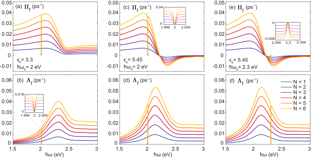
The first row of Fig. 5 depicts the spectra for $\Omega^{r}$ (when $\hbar\omega_{0}=$2\text{\,}\mathrm{eV}$$), $\Omega$ and $\eta$ for the (nonlocally modelled) case where $\epsilon_{\text{b}}=3.3$. We can readily observe that the absolute values of both $\Omega^{r}$ and $\Omega$ closely align with the respective real valued components, suggesting a minimal contribution from the respective imaginary parts. Notice again, how the shape of $\Re{\Omega}$ spectrum strikingly resembles the shape of the FWHM vs $\hbar\omega_{0}$ curve for $\epsilon_{\text{b}}=3.3$ in Fig. 4(e). Let us now recall from our formalism section that $\Omega^{r}=\Omega+\eta(\mathcal{A}-i\mathcal{B})$, extraction of the real part of which yields, $\Re{\Omega^r}=\Re{\Omega}+\Re{\eta}\mathcal{A}+\Im{\eta}\mathcal{B}$. As $\Omega$ is independent of QE contributions, the narrow Fano-shaped signature of $\Omega^{r}$ near $\omega\approx\omega_{0}$ forms mainly due to the contributions from $\Re{\eta}\mathcal{A}+\Im{\eta}\mathcal{B}$ when $\absolutevalue{\Omega^r}\approx\Re{\Omega^r}$, where $\mathcal{A}$ and $\mathcal{B}$ take the narrow Fano-like lineshapes around QE resonance we observed in Fig. 3.

If we vary $\hbar\omega_{0}$ in Fig. 5(a) from $1.5-$3\text{\,}\mathrm{eV}$$, the narrow Fano-like lineshape now observed around $\hbar\omega\approx$2\text{\,}\mathrm{eV}$$ will traverse from $\approx 1.5-$3\text{\,}\mathrm{eV}$$ without a reversal of shape. That is, the Fano-like lineshape we observed for $\mathcal{A}$ and $\mathcal{B}$, where a peak is followed by a trough, will be qualitatively retained in $\Re{\Omega^r}$’s Fano signature around QE resonance. However, as $\hbar\omega_{0}$ traverses from $1.5-$3\text{\,}\mathrm{eV}$$, the amplitude variation of the Fano peak and trough will be governed by $\Re{\eta}$ and $\Im{\eta}$ indicated in Fig. 5(c). When both $\Re{\eta}$ and $\Im{\eta}$ take large positive values, the similarly shaped Fano patterns of $\mathcal{A}$ and $\mathcal{B}$ will be linearly (additively) combined to give the enhanced Fano pattern we observe for $\Re{\Omega^r}=\Re{\Omega}+\Re{\eta}\mathcal{A}+\Im{\eta}\mathcal{B}$ around $\omega\approx\omega_{0}$ when $\hbar\omega_{0}=$2\text{\,}\mathrm{eV}$$ in Fig. 5(a). When $\hbar\omega_{0}\to$1.5\text{\,}\mathrm{eV}$$ or $3\text{\,}\mathrm{eV}$ (the two extreme points along the x-axis), the peak and trough amplitudes of $\Re{\Omega^r}$’s narrow Fano pattern will comparatively reduce due to the diminishing but positive $\Re{\eta}$ and $\Im{\eta}$ values observed in Fig. 5(c) at the two extreme ends along the x-axis. Notice how the Fano signature of $\Re{\Omega^r}$ enhances with increasing $N$ due to increased plasmonic impact, which is also explainable by the aforementioned formula for $\Re{\Omega^r}$. In essence, when both $\Re{\eta}$ and $\Im{\eta}$ are positive, the Fano signature of $\Re{\Omega^r}$ will not reverse in shape along the $x-$axis, but its magnitude will be governed by $\Re{\eta}$ and $\Im{\eta}$.

References

- Hapuarachchi (2019) H. P. Hapuarachchi, Analysis of Exciton-Plasmon Nanohybrids, Ph.D. thesis, Monash University, Clayton, Australia (2019).
- Artuso (2012) R. D. Artuso, The Optical Response of Strongly Coupled Quantum Dot-Metal Nanoparticle Hybrid Systems, Ph.D. thesis, University of Maryland, College Park, Maryland, United States (2012).
- Maier (2007) S. A. Maier, Plasmonics: fundamentals and applications (Springer Science & Business Media, 2007) Chap. 5.
- Premaratne and Agrawal (2011) M. Premaratne and G. P. Agrawal, Light propagation in gain media: optical amplifiers (Cambridge University Press, 2011).
- Hapuarachchi and Premaratne (2018) H. Hapuarachchi and M. Premaratne, in 2018 IEEE 12th International Conference on Nano/Molecular Medicine and Engineering (NANOMED) (IEEE, 2018) pp. 20–24.
- Senevirathne et al. (2019) V. Senevirathne, H. Hapuarachchi, S. Mallawaarachchi, S. D. Gunapala, M. I. Stockman, and M. Premaratne, Journal of Physics: Condensed Matter 31, 085302 (2019).
- Gettapola et al. (2019) K. Gettapola, H. Hapuarachchi, M. I. Stockman, and M. Premaratne, Journal of Physics: Condensed Matter 32, 125301 (2019).
- Sukharev and Nitzan (2017) M. Sukharev and A. Nitzan, Journal of Physics: Condensed Matter 29, 443003 (2017).
- Anker et al. (2010) J. N. Anker, W. P. Hall, O. Lyandres, N. C. Shah, J. Zhao, and R. P. Van Duyne, in Nanoscience and Technology: A Collection of Reviews from Nature Journals (World Scientific, 2010) pp. 308–319.
- Zhou et al. (2015) H. Zhou, J. Liu, and S. Zhang, TrAC Trends in Analytical Chemistry 67, 56 (2015).
- Hapuarachchi et al. (2019) H. Hapuarachchi, S. D. Gunapala, and M. Premaratne, Journal of Physics: Condensed Matter 31, 325301 (2019).
- Mallawaarachchi et al. (2018) S. Mallawaarachchi, M. Premaratne, and P. K. Maini, IEEE Journal of Selected Topics in Quantum Electronics 25, 1 (2018).
- Jayasekara et al. (2015) C. Jayasekara, M. Premaratne, M. I. Stockman, and S. D. Gunapala, Journal of Applied Physics 118, 173101 (2015).
- Gamacharige et al. (2019) D. L. Gamacharige, S. D. Gunapala, M. I. Stockman, and M. Premaratne, Physical Review B 99, 115405 (2019).
- Kumarapperuma et al. (2018) L. Kumarapperuma, M. Premaratne, P. K. Jha, M. I. Stockman, and G. P. Agrawal, Applied Physics Letters 112, 201108 (2018).
- Weeraddana et al. (2016) D. Weeraddana, M. Premaratne, S. D. Gunapala, and D. L. Andrews, Physical Review B 94, 085133 (2016).
- Abeywickrama et al. (2019) C. Abeywickrama, M. Premaratne, S. D. Gunapala, and D. L. Andrews, Journal of Physics: Condensed Matter 32, 095305 (2019).
- Tang and Sargent (2011) J. Tang and E. H. Sargent, Advanced materials 23, 12 (2011).
- Lin et al. (2015) Q. Lin, A. Armin, R. C. R. Nagiri, P. L. Burn, and P. Meredith, Nature Photonics 9, 106 (2015).
- Sadeghi (2010) S. Sadeghi, Nanotechnology 21, 355501 (2010).
- Govorov et al. (2006) A. O. Govorov, G. W. Bryant, W. Zhang, T. Skeini, J. Lee, N. A. Kotov, J. M. Slocik, and R. R. Naik, Nano letters 6, 984 (2006).
- Hartsfield et al. (2015) T. Hartsfield, W.-S. Chang, S.-C. Yang, T. Ma, J. Shi, L. Sun, G. Shvets, S. Link, and X. Li, Proceedings of the National Academy of Sciences 112, 12288 (2015).
- Zhang et al. (2019) H. Zhang, M. Li, K. Wang, Y. Tian, J.-S. Chen, K. T. Fountaine, D. DiMarzio, M. Liu, M. Cotlet, and O. Gang, ACS nano (2019).
- Nicoli et al. (2019) F. Nicoli, T. Zhang, K. Hübner, B. Jin, F. Selbach, G. Acuna, C. Argyropoulos, T. Liedl, and M. Pilo-Pais, Small 15, 1804418 (2019).
- Warnakula et al. (2019) T. Warnakula, S. D. Gunapala, M. I. Stockman, and M. Premaratne, Physical Review B 100, 085439 (2019).
- Hapuarachchi et al. (2018a) H. Hapuarachchi, S. Mallawaarachchi, H. T. Hattori, W. Zhu, and M. Premaratne, Journal of Physics: Condensed Matter 30, 054006 (2018a).
- Liu et al. (2017) Y. Liu, X. Dai, S. Mallawaarachchi, H. Hapuarachchi, Q. Shi, D. Dong, S. H. Thang, M. Premaratne, and W. Cheng, Journal of Materials Chemistry C 5, 10926 (2017).
- Hapuarachchi et al. (2017) H. Hapuarachchi, M. Premaratne, Q. Bao, W. Cheng, S. D. Gunapala, and G. P. Agrawal, Physical Review B 95, 245419 (2017).
- Ridolfo et al. (2010) A. Ridolfo, O. Di Stefano, N. Fina, R. Saija, and S. Savasta, Physical review letters 105, 263601 (2010).
- Hapuarachchi et al. (2018b) H. Hapuarachchi, S. D. Gunapala, Q. Bao, M. I. Stockman, and M. Premaratne, Physical Review B 98, 115430 (2018b).
- Hatef et al. (2012) A. Hatef, S. Sadeghi, and M. R. Singh, Nanotechnology 23, 205203 (2012).
- Raza et al. (2015) S. Raza, S. I. Bozhevolnyi, M. Wubs, and N. A. Mortensen, J. Phys. Condens. Matter 27, 183204 (2015).
- Artuso and Bryant (2008) R. D. Artuso and G. W. Bryant, Nano letters 8, 2106 (2008).
- Mortensen et al. (2014) N. A. Mortensen, S. Raza, M. Wubs, T. Søndergaard, and S. I. Bozhevolnyi, Nature communications 5, 3809 (2014).
- Tiggesbäumker et al. (1993) J. Tiggesbäumker, L. Köller, K.-H. Meiwes-Broer, and A. Liebsch, Physical Review A 48, R1749 (1993).
- Wubs and Mortensen (2017) M. Wubs and N. A. Mortensen, in Quantum Plasmonics (Springer, 2017) pp. 279–302.
- Raza et al. (2013a) S. Raza, N. Stenger, S. Kadkhodazadeh, S. V. Fischer, N. Kostesha, A.-P. Jauho, A. Burrows, M. Wubs, and N. A. Mortensen, Nanophotonics 2, 131 (2013a).
- Raza et al. (2013b) S. Raza, W. Yan, N. Stenger, M. Wubs, and N. A. Mortensen, Optics express 21, 27344 (2013b).
- Zuloaga et al. (2009) J. Zuloaga, E. Prodan, and P. Nordlander, Nano letters 9, 887 (2009).
- Andersen et al. (2012) K. Andersen, K. W. Jacobsen, and K. S. Thygesen, Physical Review B 86, 245129 (2012).
- Mallawaarachchi et al. (2017) S. Mallawaarachchi, M. Premaratne, S. D. Gunapala, and P. K. Maini, Physical Review B 95, 155443 (2017).
- Zhu et al. (2016) W. Zhu, R. Esteban, A. G. Borisov, J. J. Baumberg, P. Nordlander, H. J. Lezec, J. Aizpurua, and K. B. Crozier, Nature communications 7, 1 (2016).
- Wang et al. (2020) H. Wang, K. Chen, J. Pan, S. Huang, J. Lin, W. Xie, and X. Huang, Journal of Quantitative Spectroscopy and Radiative Transfer , 106878 (2020).
- Nordlander et al. (2004) P. Nordlander, C. Oubre, E. Prodan, K. Li, and M. Stockman, Nano letters 4, 899 (2004).
- Su et al. (2003) K.-H. Su, Q.-H. Wei, X. Zhang, J. Mock, D. R. Smith, and S. Schultz, Nano letters 3, 1087 (2003).
- Griffiths and College (1999) D. J. Griffiths and R. College, Introduction to electrodynamics, Vol. 3 (prentice Hall Upper Saddle River, NJ, 1999) Chap. 3.
- Yariv (1967) A. Yariv, Quantum electronics (Wiley, 1967).
- Blum (2012) K. Blum, Density matrix theory and applications, Vol. 64 (Springer Science & Business Media, 2012).
- Weeraddana et al. (2017) D. Weeraddana, M. Premaratne, S. D. Gunapala, and D. L. Andrews, The Journal of chemical physics 147, 074117 (2017).
- Kosionis et al. (2012) S. G. Kosionis, A. F. Terzis, V. Yannopapas, and E. Paspalakis, The Journal of Physical Chemistry C 116, 23663 (2012).
- Funston et al. (2009) A. M. Funston, C. Novo, T. J. Davis, and P. Mulvaney, Nano letters 9, 1651 (2009).
- Johnson and Christy (1972) P. B. Johnson and R.-W. Christy, Physical review B 6, 4370 (1972).