Supplementary Information for “Parallel single-shot measurement and coherent control of solid-state spins below the diffraction limit”

1 Experimental configuration

This section lays out a detailed description of our experimental setup (Fig. S1a). A tunable laser (Toptica CTL1500), stabilized to a reference cavity (Stable Laser Systems), provides a single tone optical signal $f_{\text{laser}}$ . Optical pulses are generated using an intensity modulating electro-optic modulator (IM-EOM, Lucent X-2623Y) and two acousto-optic modulators (AOMs, Isomet 1205C-1 and 1250C-868) in series. The two AOMs cumulatively provide a 142 dB optical power extinction ratio (one double-pass, one single-pass). The light enters a ³He cryostat (BlueFors LD250HE) in a single-mode optical fiber and is coupled to the PC cavity (Fig. S2) using a grating coupler [ding2013ultrahigh] with 40% one-way efficiency. The fiber end, mounted on top of a three-axis nanopositioner (Attocube), is angle-polished to guide and couple light into the grating coupler [li2014silicon]. Returning photons are separated using a 90:10 beamsplitter and detected in a superconducting nanowire single photon detector (SNSPD, Quantum Opus) in a separate, 2.2 K cryostat.

Refer to caption — FIG. S1: Experimental setup. (a) Sketch of the experimental setup. (b,c) Optical sidebands and microwave (MW) pulse generation circuit diagrams. See Sec. 1 for abbreviations. Additional component details: Amp1, Mini-Circuits ZHL-4240W+; Amp2, Mini-Circuits ZHL-30W-252+; SPDT switches, Mini-Circuits ZASWA2-50DR-FA+.

To enable fast switching of the laser frequency, we address the ions using RF sidebands generated by the IM-EOM (Fig. S1b), with a DC bias chosen to suppress the carrier transmission. The initialization and readout sequences require switching the sideband frequency on the $\sim\!100\,\mu$ s timescale, which is accomplished with a fast-switching RF generator (RF synth., Holzworth HSM6001B), while the optical phase shift pulse is generated by a separate synthesizer (RF1, SRS SG386). The spin transitions are driven with microwave magnetic fields generated by a coplanar waveguide attached to the end of the optical fiber. The ground and excited state spin transitions are driven by separate synthesizers (RF2 and RF3, respectively; SRS SG386) with signals being amplified to 21W before entering the cryostat (Fig. S1c). An arbitrary waveform generator (AWG, Agilent 33622) drives an IQ mixer that modulates the signal from RF2 to generate MW pulses with different phases for the ground state.

2 State-selective initialization of spins

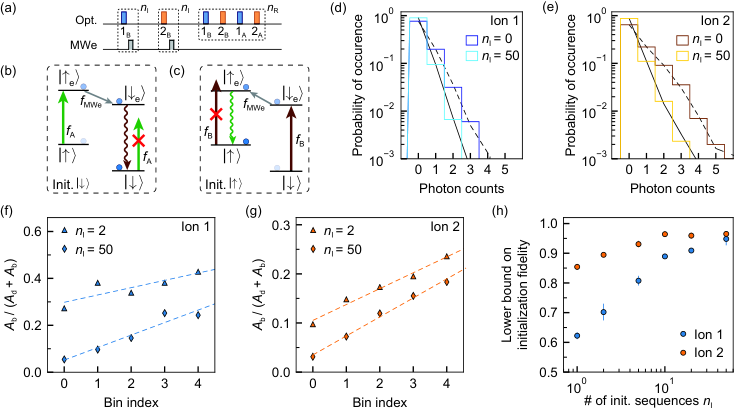
In this section, we provide a detailed characterization of the state-selective initialization protocol. A sketch of the protocol for initializing the spins is shown in Fig. S3b,c. The initialization fidelity is significantly better than the readout fidelity, such that we cannot directly probe the initialization error. To get a better estimate of the initialization fidelity, we look at the photon number distributions during the measurement while implementing the pulse sequence in Fig. S3a. In an ideal case of perfect initialization to $\left|{\uparrow}\right\rangle$ , a histogram of detected photon counts while exciting the ion using transition B exhibits a dark count-limited Poisson distribution. Imperfect initialization leads to the presence of an additional Poisson distribution with a higher mean photon count due to residual population in $\left|{\downarrow}\right\rangle$ . Representative histograms of B photons while ion 1 and ion 2 are initialized to $\left|{\uparrow}\right\rangle$ are shown in Fig. S3d,e. The data is fitted to a bimodal Poisson distribution of the form $A_{\text{d}}\exp(-\mu_{\text{d}})\mu_{\text{d}}^{x}/x!+A_{\text{b}}\exp(-\mu_{\text{b}})\mu_{\text{b}}^{x}/x!$ , where $\mu_{\text{b}},\mu_{\text{d}}$ are the mean photon counts while exciting each ion on the A,B transitions (when the ions are initialized to $\left|{\uparrow}\right\rangle$ ), and $A_{\text{b}},A_{\text{d}}$ are the fitted amplitudes of corresponding distributions. If $\mu_{\text{b}}$ is big enough that the histogram is bimodal, $A_{\text{b}}$ can be fitted with high precision.

However, finite cyclicity of the spin-conserving transitions A,B introduces a small probability ( $\propto$ $n_{\text{R}}$ , for $n_{\text{R}}\ll$ cyclicity) to flip the electron spin during the readout process. To that end, while the readout sequence involves $n_{\text{R}}=250$ pulses, we compute photon count histograms considering each group of 50 consecutive readout pulses (denoted as a “bin”) at a time, and fit the histograms to the aforementioned bimodal Poisson distribution. We conservatively interpret $A_{\text{b}}/(A_{\text{b}}+A_{\text{d}})$ to be the probability that the spin was in the wrong state at the beginning of the bin. As expected, the extracted probability value increases linearly with the bin index (Fig. S3f,g). By fitting a linear function to the data, we interpret the $y$ -intercept to be an upper bound on the initialization infidelity. We show the result of this fidelity analysis for varying number of repetitions of the initialization sequence, $n_{\text{I}}$ , in Fig. S3h, revealing initialization fidelity for ion 1 and ion 2 to be at least 95% and 97% respectively, using $n_{\text{I}}=50$ . The lower bound is limited by the finite probability of optically pumping the ion inside the first bin, and we believe that the saturated initialization fidelity should be nearly perfect, limited only by off-resonant driving of the wrong transition. The slower rate of saturation and inferior initialization fidelity of ion 1 can be attributed to its larger spectral diffusion, leading to less efficient optical excitation probability per pulse.

3 Spin coherence

We measure the ground state spin $T_{1}$ value by initializing each ion to the $\left|{\downarrow}\right\rangle$ state and performing spin readout at varying delay times ( $t_{\text{delay}}$ ); a single exponential fit to the data gives $T_{1}$ of $19.9\pm 4.1$ seconds and $23.3\pm 1.3$ seconds for ion 1 and ion 2, respectively (Fig. S4a). Ramsey measurements reveal $T_{2}^{*}$ of $88\pm 9$ ns and $94\pm 6$ ns, respectively, extracted from fitting a single exponential to the data (Fig. S4b). For the optical phase control, we embed optical pulses within an XY8 sequence. The coherence decay during an XY8 sequence of total length $t$ is well-described by a Gaussian $\exp[-(t/T_{2})^{2}]$ with $T_{2,\text{XY8}}$ of $16.5\pm 0.5$ $\mu$ s and $15.3\pm 0.3$ $\mu$ s.

We have not measured the spin coherence of ions 3 – 6 in the course of this work, but note that the spin of ion 5 was partially characterized in Ref. [raha2020] at a slightly different magnetic field orientation (in that work, it was referred as “ion 3”), with values of $T_{1}=45\pm 4$ seconds, $T_{2}^{*}=125\pm 5$ ns, $T_{\text{2,Hahn echo}}=3.3\pm 0.2$ $\mu$ s.

4 Single qubit gates

4.1 Theory of ion-selective phase-shifts and loss of visiblity

We apply detuned optical pulses to accumulate phase shift using AC Stark effect. Consider the atom as a two-level system { $\left|{g}\right\rangle$ , $\left|{e}\right\rangle$ } with a transition splitting of $\hbar\omega_{0}$ , driven by a laser at frequency $\omega$ . Under the dipole approximation, the effective non-Hermitian Hamiltonian in the rotating frame of the laser field (making the rotating-wave approximation) is given by:

H=\frac{\hbar\Omega}{2}(\left|{g}\right\rangle\left\langle{e}\right|+\left|{e}\right\rangle\left\langle{g}\right|)-\hbar(\Delta+i\Gamma/2)\left|{e}\right\rangle\left\langle{e}\right|,

(S1)

where $\Omega$ is the Rabi frequency, $\Delta=\omega-\omega_{0}$ is the detuning of the optical drive from the transition frequency, and $\Gamma$ is the spontaneous emission rate. The perturbed ground state and its corresponding energy shift are:

\left|{\psi}\right\rangle=\left|{g}\right\rangle+\frac{\sqrt{(\Delta+i\Gamma/2)^{2}+\Omega^{2}}-(\Delta+i\Gamma/2)}{\Omega}\left|{e}\right\rangle\approx\left|{g}\right\rangle+\frac{\Omega}{2(\Delta+i\Gamma/2)}\left|{e}\right\rangle

(S2)

\Delta E=\text{Re}\left\{\frac{\hbar}{2}\left[\sqrt{(\Delta+i\Gamma/2)^{2}+\Omega^{2}}-(\Delta+i\Gamma/2)\right]\right\}\approx\hbar\frac{\Omega^{2}}{4}\frac{\Delta}{\Delta^{2}+\Gamma^{2}/4}

(S3)

for $\Omega\ll\sqrt{\Delta^{2}+\Gamma^{2}/4}$ . For a given laser frequency, the two spin-conserving transitions A,B of an Er³⁺ ion experience dissimilar detunings, denoted by $\Delta_{\text{A}},\Delta_{\text{B}}$ . However, $\Omega$ must be the same for the two transitions since the spin states originating from the same doublet are related to each other via time-reversal symmetry [raha2020]. Treating these transitions as two independent two-level systems, the net phase shift imprinted between $\left|{\downarrow}\right\rangle$ and $\left|{\uparrow}\right\rangle$ resulting from the detuned optical pulse is:

\phi=T\frac{\Omega^{2}}{4}\left(\frac{\Delta_{\text{B}}}{\Delta_{\text{B}}^{2}+\Gamma^{2}/4}-\frac{\Delta_{\text{A}}}{\Delta_{\text{A}}^{2}+\Gamma^{2}/4}\right),

(S4)

where $T$ is the optical pulse width. On the other hand, due to mixing of $\left|{e}\right\rangle$ in the perturbed ground state (Eq. S2), there is a possibility of spontaneous emission from the excited state, which reduces the visibility ( $\mathcal{V}$ ) of the fringes in the phase shift measurements. This can be calculated perturbatively from the excited state population $\Omega^{2}/(4\Delta^{2}+\Gamma^{2})$ for each transition as:

\Delta\mathcal{V}=1-\exp\left[-T\Gamma\frac{\Omega^{2}}{4}\frac{1}{2}\left(\frac{1}{\Delta_{\text{A}}^{2}+\Gamma^{2}/4}+\frac{1}{\Delta_{\text{B}}^{2}+\Gamma^{2}/4}\right)\right].

(S5)

For far-detuned optical drive pulses ( $\Delta_{\text{A}},\Delta_{\text{B}}\gg\Gamma$ ), Eq. S4 and S5 reduces to the following forms:

\phi=T\frac{\Omega^{2}}{4}\left(\frac{1}{\Delta_{\text{B}}}-\frac{1}{\Delta_{\text{A}}}\right),\quad\quad\Delta\mathcal{V}=1-\exp\left[-T\Gamma\frac{\Omega^{2}}{4}\frac{1}{2}\left(\frac{1}{\Delta_{\text{A}}^{2}}+\frac{1}{\Delta_{\text{B}}^{2}}\right)\right].

(S6)

4.2 Linewidth broadening

In our experiments, the observed linewidth is more than two orders of magnitude broader than the spontaneous emission rate, presumably because of spectral diffusion. While the calculation above estimates the loss of coherence from radiative decay of the excited state, the spin can also dephase from fluctuations in the optical transition frequency that cause uncertainty in the AC Stark shift. From numerical simulations of the master equation (Fig. S5), we find that the functional form of the loss of coherence (Eq. S5) is identical for the following cases: pure radiative decay, pure dephasing, or slow diffusion of the transition with a Lorentzian probability distribution. If multiple processes are present, the functional form is unchanged and their (Lorentzian) linewidths sum. Conversely, slow diffusion with a Gaussian probability distribution gives rise to a different line shape. In the experiment, we do not probe the loss or lineshape with sufficient precision to distinguish these cases.

4.3 Simultaneous arbitrary rotations on two qubits

Universal control of a single qubit requires arbitrary rotations around two orthogonal axes. MW control alone imparts arbitrary but identical rotations on all spin qubits since it addresses the spins globally. In this section, we theoretically show that arbitrary rotations on multiple spins can be achieved by combining MW rotations and ion-selective optical $z$ rotations.

We start with the simple case of two qubits. Arbitrary unitary operations on two qubits of the form $U\otimes U^{\prime}$ can be decomposed into two consecutive operations $U\otimes\mathbb{I}$ and $\mathbb{I}\otimes U^{\prime}$ . First, let’s implement the operation $U\otimes\mathbb{I}$ . Consider the following quantum circuit: